Antimatter Regions in the Early Universe and Big Bang Nucleosynthesis

Abstract

We have studied big bang nucleosynthesis in the presence of regions of antimatter. Depending on the distance scale of the antimatter region, and thus the epoch of their annihilation, the amount of antimatter in the early universe is constrained by the observed abundances. Small regions, which annihilate after weak freezeout but before nucleosynthesis, lead to a reduction in the ${}^{4}{\rm He}$ yield, because of neutron annihilation. Large regions, which annihilate after nucleosynthesis, lead to an increased ${}^{3}{\rm He}$ yield. Deuterium production is also affected but not as much. The three most important production mechanisms of ${}^{3}{\rm He}$ are (1) photodisintegration of ${}^{4}{\rm He}$ by the annihilation radiation, (2) $\bar{\rm p}{}^{4}{\rm He}$ annihilation, and (3) $\bar{\rm n}{}^{4}{\rm He}$ annihilation by “secondary” antineutrons produced in ${}^{4}\overline{\rm He}$ annihilation. Although $\bar{\rm p}{}^{4}{\rm He}$ annihilation produces more ${}^{3}{\rm He}$ than the secondary $\bar{\rm n}{}^{4}{\rm He}$ annihilation, the products of the latter survive later annihilation much better, since they are distributed further away from the annihilation zone. Our results are in qualitative agreement with similar work by Rehm and Jedamzik, but we get a larger ${}^{3}{\rm He}$ yield.

HIP-2000-31/TH

I Introduction

A Antimatter in the Universe

The local universe is baryon asymmetric. It contains matter, not antimatter. In standard homogeneous big bang cosmology the universe was filled with a uniform mixture of antimatter and matter very early on, with a slight excess of matter over antimatter. This excess of matter was left over when matter and antimatter annihilated during the first millisecond.

This baryon asymmetry is characterized by the baryon-to-photon ratio,

$$\eta\equiv\frac{n_{b}-n_{\bar{b}}}{n_{\gamma}}\equiv\frac{n_{B}}{n_{\gamma}},$$ (1)

where $n_{b}$ is the number density of baryons and $n_{\bar{b}}$ the number density of antibaryons.

There are many proposed mechanisms for baryogenesis to explain the origin of this asymmetry. The simplest versions of baryogenesis produce a homogeneous asymmetry, but there are many possibilities for inhomogeneous baryogenesis, which could produce a baryon excess in some regions and an antibaryon excess in other regions. This leads to a structure of matter and antimatter regions after local annihilation during the first millisecond.

In scenarios connected with inflation, there is no a priori constraint on the distance scale of these matter and antimatter regions. If the distance scale is small, the antimatter regions would have annihilated in the early universe, and the presence of matter today requires asymmetric baryogenesis, producing more baryons than antibaryons. If the distance scale is large, antimatter regions would have survived till present.

In the latter case, an overall baryon symmetry remains a possibility. The universe could contain equal amounts of matter and antimatter, spatially separated into matter and antimatter domains. In this case, the absence of observed annihilation radiation from the domain boundaries indicates that the typical size of these domains would have to be very large.

Considering only the conditions in the present universe, the lower limit to the domain size corresponds to the scale of cluster of galaxies, of the order of 20 Mpc[3]. Because of the low density of intergalactic space between clusters the annihilation radiation between a cluster and an “anticluster” could have escaped detection.

However, the isotropy of the cosmic microwave background (CMB) rules out large voids between matter and antimatter regions during an earlier time. Thus annihilation would have been more intense before structure formation. The relic $\gamma$ rays would contribute to the cosmic diffuse gamma (CDG) spectrum. The observed CDG spectrum gives a much larger lower limit to the domain size, of the order of $10^{3}$ Mpc, comparable to the size of the visible universe[4]. A boundary of an even larger domain intersecting the last scattering surface could leave an imprint on the CMB[5], but these are unlikely to be observable with planned CMB probes[6].

If we drop the assumption of baryon symmetry, allowing for a lesser amount of antimatter than matter, then instead of a lower limit to the domain size, observations just place upper limits to the antimatter-matter ratio $R$ at different distance scales. Indeed, it may be possible to have a small fraction $R<10^{-6}$ of antimatter stars in our galaxy[7].

No antinuclei (with $|Z|>1$) have ever been observed in cosmic rays. The Alpha Magnetic Spectrometer (AMS)[8] to be placed on the International Space Station will look for antinuclei in cosmic rays, and if none are found, will place a tight upper limit on the antimatter fraction of cosmic ray sources. The AMS precursor flight on the Space Shuttle observed $2.86\times 10^{6}$ helium nuclei but no antihelium[9], giving an upper limit $\overline{\rm He}/{\rm He}<1.1\times 10^{-6}$ on the antihelium-helium flux ratio in cosmic rays.

B Inhomogeneous baryogenesis

Early work on antimatter regions in the universe (see the review by Steigman[3]) considered them as an initial condition for the universe[10], or tried to form them by separating matter from antimatter at a later stage[11]. Later work is related to scenarios for inhomogeneous baryogenesis.

There are many proposed mechanisms for baryogenesis, including grand unified theory (GUT) baryogenesis, electroweak baryogenesis, and Affleck-Dine baryogenesis. The simplest versions produce a homogeneous baryoasymmetry, but simple modifications lead to an inhomogeneous baryogenesis which produces matter and antimatter regions[12, 13, 14, 15, 16]. See, e.g., the reviews by Dolgov[17].

Inhomogeneous baryogenesis without inflation leads to a matter-antimatter domain structure with a very small distance scale. Models connected to inflation can lead to arbitrarily large distance scales. Some scenarios for GUT baryogenesis lead to an unacceptable large domain wall energy between the matter and antimatter domains, but other scenarios avoid this problem[13].

Most studies of inhomogeneous baryogenesis have been for a globally baryon symmetric universe. As it has been recently shown[4] that the distance scale in this case would have to be at least comparable to the present horizon, the attention has shifted to models where the observable universe is baryon asymmetric, but could contain a smaller amount of antimatter[18, 19].

C Antimatter regions in the early universe

On scales smaller than about 1 kpc[20], antimatter regions would have annihilated by now but could have left an observable signature in the CDG spectrum, in the CMB spectrum, or in the yields of light elements from big bang nucleosynthesis (BBN).

The smaller the size of the antimatter regions, the earlier they annihilate. Domains smaller than 100 m at $T=$ 1 MeV, corresponding to a comoving (present) scale of $6\times 10^{8}$ km or 0.02 mpc, would annihilate well before nucleosynthesis and would leave no observable remnant.

The energy released in antimatter annihilation thermalizes with the ambient plasma and the background radiation, if the energy release occurs at $T>1$ keV. If the annihilation occurs later, Compton scattering between electrons heated by the annihilation and the background photons transfers energy to the microwave background, but is not able to thermalize this energy (because Compton scattering conserves photon number). The lack of observed distortion in the CMB spectrum constrains the energy release occurring after $T=1$ keV to below $6\times 10^{-5}$ of the CMB energy[21]. This leads to progressively stronger constraints on the amount of antimatter annihilating at later times, as the ratio of matter and CMB energy density is getting smaller. Above $T\sim 0.2$ eV the baryonic matter energy density is smaller than the CMB energy density, so the limits on the antimatter fraction annihilating then are weaker than $6\times 10^{-5}$.

For scales larger than about 100 pc (or $7\times 10^{11}$ m at 1 keV) the tightest constraints on the amount of antimatter come from the CMB spectral distortion, and from the CDG spectrum for even larger scales[4].

We consider here intermediate distance scales, where most of the annihilation occurs shortly before or during nucleosynthesis, or after nucleosynthesis but before recombination, at temperatures between 1 MeV and 1 eV. The strongest constraints on the amount of antimatter at these distance scales will come from big bang nucleosynthesis affected by the annihilation process.

D BBN with antimatter

Much of the early work on BBN with antimatter[3, 22, 23, 24] was either in the context of a baryon symmetric universe[22] or for a homogeneous injection of antimatter through some decay process[24].

Rehm and Jedamzik[25] studied small antimatter regions, which annihilate before nucleosynthesis, at temperatures $T>80\mbox{ keV}$. Because of faster diffusion of neutrons and antineutrons (as compared to protons and antiprotons), annihilation reduces the net neutron number, leading to underproduction of ${}^{4}{\rm He}$[3]. This sets a limit $R<10^{-2}$ for the amount of antimatter in regions of size $r_{A}\sim 1$ cm at $T=$ 100 GeV (2 km at $T=1\mbox{ MeV}$ or $3\times 10^{6}$ m at $T=1\mbox{ keV}$). Our results for these small scales agree with[25].

We consider also larger antimatter regions, which annihilate mainly during or after nucleosynthesis. We have done detailed inhomogeneous nucleosynthesis calculations, where diffusion, annihilation, and nucleosynthesis all happen simultaneously.

The case where annihilation occurs after nucleosynthesis was considered in[23]. Because annihilation of antiprotons on helium would produce D and ${}^{3}{\rm He}$ it was estimated that the observed abundances of these isotopes place a comparable upper limit to the amount of antimatter annihilated after nucleosynthesis. As we explain below, the situation is rather more complicated.

We reported our first results in[26], where we had not included some features whose effect we estimated to be small. These included (1) antinucleosynthesis in the antimatter region, (2) photodisintegration of other isotopes than ${}^{4}{\rm He}$, and (3) the dependence of the electromagnetic cascade spectrum on the initial photon spectrum from annihilation. We have now made the following changes to our computer code to take these effects into account.

(1) We have added all antinuclei up to $\bar{A}=4$ and their antinucleosynthesis. Annihilation of these antinuclei produce energetic antimatter fragments which may penetrate deep into the matter region and annihilate there. Thus annihilation reactions occur also far away from the matter-antimatter boundary.

(2) We have added photodisintegration of the lighter nuclei, D, ${}^{3}{\rm H}$, and ${}^{3}{\rm He}$.

(3) We treat photodisintegration in more detail, especially at lower temperatures, where use of the standard cascade spectrum is no longer appropriate.

Below, all distance scales given in meters will refer to comoving distance at $T=1$ keV. One meter at $T=1$ keV corresponds to $4.24\times 10^{6}$ m or $1.37\times 10^{-10}$ pc today. Rehm and Jedamzik[25] give their distance scales at $T=100$ GeV. Our distances are thus larger by a factor $3.0\times 10^{8}$. We use $\hbar=c=k_{B}=1$ units.

The physics of the annihilation of antimatter regions in the early universe is discussed in Sec. II. We describe our numerical implementation in Sec. III and give the results in Sec. IV. We summarize our conclusions in Sec. V.

II Annihilation of Antimatter Domains

A Mixing of matter and antimatter

Consider the evolution of an antimatter region, with radius $r_{A}$, surrounded by a larger region of matter. We are interested in the period in the early universe when the temperature was between 1 MeV and 1 eV (age of the universe between 1 s and 30000 years). The universe is radiation dominated during this period. At first matter and antimatter are in the form of nucleons and antinucleons, after nucleosynthesis in the form of ions and anti-ions. Matter and antimatter are mixed by diffusion at the boundary and annihilated. Thus there will be a narrow annihilation zone separating the matter and antimatter regions.

Before nucleosynthesis the mixing of matter and antimatter occurs mainly through neutron/antineutron diffusion, since neutrons diffuse much faster than protons. If the radius of the antimatter region is less than $r\approx 10^{7}$ m, all antimatter annihilates before nucleosynthesis. In nucleosynthesis the remaining free neutrons go into ${}^{4}{\rm He}$ nuclei. The mixing of matter and antimatter practically stops until the density has decreased enough for ion diffusion to become effective at $T\approx 3$ keV.

Thus there are two stages of annihilation, the first one before nucleosynthesis, at $T\gtrsim 70$ keV, the second well after nucleosynthesis, at $T\lesssim 3$ keV. The physics during the two regimes is quite different. The first regime was discussed in[25]. We concentrate on the second regime in the following discussion.

Hydrodynamic expansion becomes important at $T\approx 30$ keV. At that time the annihilation of thermal electron-positron pairs becomes practically complete and the photon mean free path increases rapidly. When the mean free path becomes larger than the distance scale of the baryon inhomogeneity, the baryons stop feeling the pressure of the photons, which had balanced the pressure of baryons and electrons. The pressure gradient then drives the fluid into motion towards the annihilation zone[27, 28]. This flow is resisted by Thomson drag. The fluid reaches a terminal velocity [28]

$$v=\frac{3}{4\sigma_{T}\varepsilon_{\gamma}|n_{e}^{\ast}|}\frac{dP}{dr}.$$ (2)

Here $\varepsilon_{\gamma}$ is the energy density of photons, $\sigma_{T}=0.665\times 10^{-28}{\rm m}^{2}$ is the Thomson cross section, $P$ is the pressure of baryons and electrons, and $n_{e}^{\ast}=n_{e^{-}}-n_{e^{+}}$ is the net electron density. With $P\approx(n_{B}+n_{e})T$ and $|n_{e}^{\ast}|\approx n_{B}$, we get a diffusive equation

$$\frac{\partial n_{B}}{\partial t}=\nabla\cdot\left(\frac{3T}{2\sigma_{T}\varepsilon_{\gamma}}\nabla n_{B}\right)$$ (3)

for the baryon density, with an effective baryon diffusion constant due to hydrodynamic expansion

$$D_{\rm hyd}=\frac{3T}{2\sigma_{T}\varepsilon_{\gamma}}\propto T^{-3}.$$ (4)

The hydrodynamic expansion alone does not cause mixing, but it significantly speeds up annihilation by bringing material towards the annihilation zone. The annihilation zone is surrounded by a depletion zone[4], where the density of (anti)matter has decreased due to matter flow into the annihilation zone. The resulting pressure gradient maintains this flow.

Antinucleosynthesis in the antimatter region produces antinuclei. The yields of these anti-isotopes are not interesting in themselves, since they are eventually annihilated. The annihilation of these antinuclei with nucleons produces energetic antinucleons and lighter antinuclei, which may penetrate deep into the matter region before annihilating. Thus, in addition to “primary” annihilation in the annihilation zone, there is also “secondary” annihilation outside this zone.

B Annihilation reactions

The primary annihilation reactions occur at low energies where reaction data is scarce or non-existent. Theoretically, the annihilation cross section is known to behave as $1/v$, when one or both of the annihilating particles are neutral, and as $1/v^{2}$ when both are charged.

More precisely, the theoretical $\bar{\rm n}{\rm A}$ cross section is[29, 30]

$$\sigma\approx 4\pi\biggl{(}\frac{\mbox{Im}(-a_{s})}{q}-2\mbox{Im}^{2}(-a_{s})\biggr{)},$$ (5)

where $a_{s}$ is the scattering length, $q=\mu v$, $\mu$ is the reduced mass, and $v$ is the relative velocity of the annihilating particles.

The analogous expression for S-wave $\bar{\rm p}{\rm A}$ annihilation is[31, 30]

$$\sigma = \frac{8\pi^{2}}{1-\exp(-2\pi\eta)}\frac{1}{q^{2}}\frac{\mbox{Im}(-a_{\rm sc}/B)}{|1+iqw(\eta)a_{\rm sc}|^{2}}$$ (6)

$$\approx C(v)\frac{4\pi}{q}\frac{\mbox{Im}(-a_{\rm sc})}{|1+i2\pi a_{\rm sc}/B|^{2}},$$ (7)

where $\eta=-1/qB$ is the dimensionless Coulomb parameter, $B=1/Z\mu\alpha$ is the Bohr radius of the antiparticle-particle system, $a_{\rm sc}$ is the Coulomb-corrected scattering length and

$$C(v)\equiv\frac{2\pi Z\alpha/v}{1-\exp(-2\pi Z\alpha/v)}.$$ (8)

There is laboratory data only for some of the relevant scattering lengths, and the uncertainties are large[32, 33]. From atomic data[34, 35, 30], the $\bar{\rm p}{\rm p}$ system has $\mbox{Im}(-a_{\rm sc})=0.71\pm 0.05$ fm. Recent experimental data by the OBELIX group[36] gives $\mbox{Im}(-a_{\rm sc})=0.62\pm 0.02\pm 0.04$ fm for $\bar{\rm p}{\rm D}$ and $\mbox{Im}(-a_{\rm sc})=0.36\pm 0.03^{+0.19}_{-0.11}$ for $\bar{\rm p}{}^{4}{\rm He}$.

Primary annihilation is not sensitive to the annihilation cross sections, since annihilation is complete in the annihilation zone anyway. In secondary annihilation the $A$-dependence of the annihilation cross section is important, since it determines whether antinucleons annihilate with protons, which leads to no nuclear yields, or with ${}^{4}{\rm He}$, producing ${\rm D}$ and ${}^{3}{\rm He}$.

The yields of the annihilation reactions are important. Fortunately there is data on the most important reaction, antiprotons on helium[37], and also on some other reactions with antiprotons[38, 39].

The annihilation reaction between an antinucleon and a nucleus can be thought of as an annihilation of one of the nucleons in the nucleus. According to experimental data, an antiproton is twice as likely to annihilate on a proton than on a neutron in the nucleus[40, 41].

The annihilation of a nucleon and an antinucleon produces a number of pions, on average 5–6 with a third of them neutral[3, 41]. The charged pions decay into muons and neutrinos, the muons into electrons and neutrinos. The neutral pions decay into two photons. About half of the annihilation energy, 1880 MeV, is carried away by the neutrinos, one third by the photons, and one sixth by electrons and positrons.

When an antinucleon annihilates on a nucleus, some of the produced pions may knock out some of the other nucleons, or in the case of larger nuclei, small fragments (p, ${\rm D}$, ${}^{3}{\rm H}$, ${}^{3}{\rm He}$, ${}^{4}{\rm He}$). Some of the annihilation energy will go into the kinetic energy of these particles and the recoil energy of the residual nucleus. Typical energies are of order $\sim 10$ MeV.

According to Balestra et al.[37] the average yields of low-energy $\bar{\rm p}{}^{4}{\rm He}$ annihilation are $0.210\pm$0.009 ${}^{3}{\rm He}$, $0.437\pm$0.032 ${}^{3}{\rm H}$, 0.07–0.19 D. This leaves about 0.7–0.9 nucleons.

Experimental data on the energy spectra of these emitted nucleons and fragments can be approximated by $Ce^{-E/E_{0}}$, where the average energy $E_{0}$ decreases with the mass of the emitted particle. However the corresponding momentum is close to 350 MeV/$c$ independent of mass[41]. The momenta of the residual nuclei are smaller. Balestra et al.[37] report a measurement on the momentum distribution of ${}^{3}{\rm He}$ from $\bar{\rm p}{}^{4}{\rm He}$ annihilation, with the mean energy corresponding to a momentum of 198 MeV/$c$. Because of their large momenta these reaction products get spread over a large area, many of them escaping the annihilation zone, at least for a while.

C Thermalization of annihilation products

The annihilation products lose their kinetic energy through collisions in the ambient plasma. Ions lose energy by Coulomb scattering on electrons and ions and by Thomson scattering on photons. If the velocity of the ion is greater than thermal electron velocities, the energy loss is mainly due to electrons. At low energies scattering on ions becomes important.

For an ion with $E\gg T$, we find that the energy loss per unit distance due to Coulomb collisions is

$$\frac{dE}{dr}= 4\pi n(Zz\alpha)^{2}\Lambda\left(1+\frac{m}{M}\right)\frac{M}{m}\frac{1}{E}\times$$ (10)

$$\Bigg{[}\sqrt{\frac{mE}{\pi MT}}\exp\left(-\frac{mE}{MT}\right)-\frac{1}{2}{\rm erf}\left({\sqrt{\frac{mE}{MT}}}\right)\Bigg{]}.$$

Here $M$, $Z$, and $E$ are the mass, charge and energy of the incoming ion, $T$ is the temperature of the plasma, $m$, $z$, and $n$ are the mass, charge, and number density of the plasma particles, and $\Lambda\sim 15$ is the Coulomb logarithm. We assumed here that both the incoming ion and the plasma particles are non-relativistic.

When the ion velocity is large compared to the thermal velocities of plasma particles, Eq. (10) simplifies into [42]

$$\frac{dE}{dr}\approx-2\pi n(Zz\alpha)^{2}\Lambda\left(1+\frac{m}{M}\right)\frac{M}{m}\frac{1}{E},$$ (11)

and in the opposite case, [$mE/(MT)\ll 1$], into[43]

$$\frac{dE}{dr}\approx-\frac{8\sqrt{\pi}}{3}n(Zz\alpha)^{2}\Lambda\left(1+\frac{m}{M}\right)\frac{1}{T}\sqrt{\frac{mE}{MT}}.$$ (12)

The energy loss in a plasma consisting of electrons and nuclei is thus

$$\frac{dE}{dr}= 4\pi n_{e}(Z\alpha)^{2}\Lambda_{e}\frac{M}{m_{\rm e}}\frac{1}{E}\times$$ (15)

$$\Bigg{[}\sqrt{\frac{m_{\rm e}E}{\pi MT}}\exp\left(-\frac{m_{\rm e}E}{MT}\right)-\frac{1}{2}{\rm erf}\left(\sqrt{\frac{m_{\rm e}E}{MT}}\right)$$

$$-\frac{1}{2}\sum_{i}\left(1+\frac{A_{i}}{A}\right)\frac{Z_{i}^{2}}{A_{i}}\frac{\Lambda_{i}}{\Lambda_{e}}\frac{m_{\rm e}}{m_{p}}\frac{n_{i}}{n_{e}}\Bigg{]}$$

where we assumed $m_{\rm e}/M\ll 1$, and used approximation (11) for scattering on nuclei. The index $i$ labels different species of nuclei in the plasma.

We plot the penetration distance $d$ of ${}^{3}{\rm He}$ and ${}^{3}{\rm H}$ ions in a homogeneous plasma in Fig.1, as a function of $E/T$, in the absence of thermal electron-positron pairs. At large energies $d\propto E^{2}$, which corresponds to approximation (11). We show also the effect of ignoring scattering on nuclei.

The drag force exerted on the ion by photons is

$$\frac{dE}{dr}=-\frac{4}{3}\left(\frac{m_{\rm e}}{M}\right)^{2}Z^{4}\sigma_{T}\varepsilon_{\gamma}v.$$ (16)

The effect of this is negligible compared to Coulomb scattering.

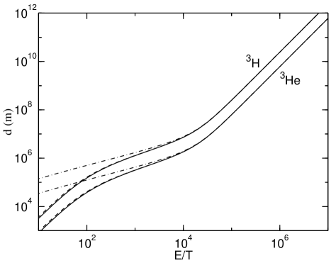
FIG. 1.: The penetration distance of a ${}^{3}{\rm He}$ and a ${}^{3}{\rm H}$ ion in matter with constant baryon density, $\eta=6\times 10^{-10}$. The distance $d$ is given in comoving units at $T=1$ keV. The solid line is for a case where all baryons are in form of protons, and the dashed line for a ${}^{4}{\rm He}$ mass fraction of 0.25. The dot-dashed line shows the effect of ignoring scattering on nuclei. The penetration distance for an ion with charge $Z$ and mass number $A$ is obtained approximately by scaling the ${}^{3}{\rm H}$ curve by a factor $A/(3Z^{2})$ vertically and by $A/3$ horizontally. For scattering on electrons (dot-dashed line) this scaling rule is exact.

Neutrons lose energy through scattering on ions and electrons. Scattering on electrons is not important for $T<30$ keV. The neutron loses a substantial part of its energy in each collision with an ion. The penetration distance is of order of the mean free path $\lambda=1/(\sigma n)$. Assuming $\eta=6\times 10^{-10}$, we find for neutron-proton scattering $\lambda\approx 4.7\times 10^{9}{\rm~{}m~{}}(T/\mbox{ keV})^{-2}$ for a neutron with a typical 70 MeV energy. At $T<0.36\mbox{ keV}$ the mean free time of a 70 MeV neutron becomes larger than its lifetime. The neutron is then likely to decay into a proton before thermalizing.

D Photodisintegration

The high-energy photons and electrons from pion decay initiate electromagnetic cascades[44, 45, 46, 47, 48, 49, 50]. The dominant thermalization mechanisms for energetic photons and electrons are photon-photon pair production and inverse Compton scattering

$$\gamma+\gamma_{bb}\rightarrow e^{+}+e^{-},\quad e+\gamma_{bb}\rightarrow e^{\prime}+\gamma^{\prime},$$ (17)

with the background photons $\gamma_{bb}$. The cascade proceeds rapidly until the photon energies $E_{\gamma}$ are below the threshold for pair production,

$$E_{\gamma}\epsilon_{\gamma}=m_{\rm e}^{2},$$ (18)

where $\epsilon_{\gamma}$ is the energy of the background photon.

Because of the large number of background photons, a significant number of them have energies $\gg T$, and the photon-photon pair production is the dominant energy loss mechanism for cascade photons down to[47]

$$E_{\rm max}=\frac{m_{\rm e}^{2}}{22T}.$$ (19)

Below this threshold energy, the dominant scattering process is photon-photon scattering down to[46]

$$E_{\rm c}=\frac{m_{\rm e}^{2}}{80T}.$$ (20)

Below this energy the dominating energy loss processes for photons are pair production on nuclei and Compton scattering on electrons. Inverse Compton scattering is still the dominant energy loss mechanism for electrons.

When energy is released in the form of photons and electrons with energies well above $E_{\rm max}$, the energy is rapidly converted into a cascade photon spectrum, which depends only on the total energy $E_{0}$ injected, and is well approximated by[47, 49]

$$\frac{dn_{\gamma}}{dE}=\left\{\begin{array}[]{ll}A(E/E_{c})^{-1.5},&E<E_{c}\\ A(E/E_{c})^{-5},&E_{c}<E<E_{\rm max}.\\ \end{array}\right.$$ (21)

The normalization factor is

$$A=\frac{3E_{0}E_{c}^{-2}}{7-(E_{c}/E_{\rm max})^{3}}.$$ (22)

Photon-photon pair production and scattering, and inverse Compton scattering, are very rapid processes compared to interactions on matter, due to the large number of photons. When the photon energies fall below $E_{c}$ the mean interaction time rises drastically. The thermalization continues through Compton scattering and pair production in the field of a nucleus, in a time scale long compared with that of the cascade. The pair production cross section is [51]

$$\sigma_{\rm pair}=\frac{3\alpha}{8\pi}Z^{2}\sigma_{T}(\frac{28}{9}\ln\frac{2E}{m_{\rm e}}-\frac{218}{27})$$ (23)

and the Compton cross section is ($E\gg m_{\rm e}$)

$$\sigma_{C}=\frac{3}{8}\sigma_{T}\frac{m_{\rm e}}{E}(\frac{1}{2}+\ln\frac{2E}{m_{\rm e}}).$$ (24)

Photons with $E>19.9\mbox{ MeV}$ disintegrate ${}^{4}{\rm He}$, producing ${}^{3}{\rm He}$, and also D for $E>26.2\mbox{ MeV}$. Above the energy $E_{\rm max}$ the cascade proceeds so rapidly that photodisintegration of nuclei is rare and can be ignored. The photodisintegration of ${}^{4}{\rm He}$ begins at $T=$ 0.6 keV, when $E_{\rm max}$ becomes larger than the binding energy of ${}^{4}{\rm He}$. For $T=0.45$–$0.60\mbox{ keV}$ ${}^{4}{\rm He}$ photodisintegration produces ${}^{3}{\rm He}$ (or ${}^{3}{\rm H}$) only, below $T=0.45\mbox{ keV}$ also ${\rm D}$ is produced, although with a smaller cross section. The photodisintegration of D begins earlier, at $T=5.3$ keV, because of the smaller deuteron binding energy. The ${}^{3}{\rm He}$ photodisintegration begins at $T=2.2\mbox{ keV}$, ${}^{3}{\rm H}$ at $T=1.9\mbox{ keV}$, and ${}^{7}{\rm Li}$ at $T=4.7\mbox{ keV}$.

During the second stage of annihilation, the mean free path of a photon at a given temperature is always larger than the distance scale of antimatter regions which annihilate at that temperature. We can therefore assume that the photons are uniformly distributed over space.

E Spectrum of annihilation photons and electrons

As the temperature falls the cascade spectrum moves to higher energies and, for $T\lesssim 100\mbox{ eV}$, it begins to overlap the initial photon spectrum from annihilation. Then the lower part of this initial spectrum is no more converted to a cascade spectrum before photodisintegration, and the shape of the initial photon spectrum becomes important.

In the pion’s rest frame its direct decay products, photons, muons, and muon neutrinos, have a single-valued energy, determined by conservation of energy and momentum. The muon decays via $\mu^{-}\rightarrow e^{-}+\nu_{\mu}+\bar{\nu}_{\rm e}$. The spectrum of the electron in the muon’s rest frame is[52]

$$\frac{dn_{e}}{dE}=16\frac{E^{2}}{m_{\mu}^{3}}\left(3-\frac{4E}{m_{\mu}}\right),\quad 0<E<\frac{1}{2}m_{\mu}\quad\hbox{(c.m.)}$$ (25)

in the approximation $m_{\rm e}/m_{\mu}\approx 0$.

For the decay products of a moving pion, integration over directions yields an energy spectrum. The decay ($\pi^{\pm}\rightarrow\mu^{\pm}+\nu_{\mu}$) of a charged pion with velocity $v_{\pi}$ and total energy $E_{\pi}$ produces a muon with a uniform spectrum in the range

$$\frac{1}{2}E_{\pi}\biggl{\{}\biggl{[}1+\biggl{(}\frac{m_{\mu}}{m_{\pi}}\biggr{)}^{2}\biggr{]}\pm v_{\pi}\biggl{[}(1-\biggl{(}\frac{m_{\mu}}{m_{\pi}}\biggr{)}^{2}\biggr{]}\biggr{\}}.$$ (26)

Similarly, the energy of a photon from neutral pion decay ($\pi^{0}\rightarrow\gamma\gamma$) has a uniform distribution in the range $\frac{1}{2}E_{\pi}(1\pm v_{\pi})$. For a muon moving with velocity $v$ and energy $E_{\mu}$, the electron spectrum becomes

$$\frac{dn_{e}}{dE}=$$ (28)

$$\frac{1}{vE_{\mu}}\left(\frac{5}{3}-12\frac{E^{2}E_{\mu}^{2}}{m_{\mu}^{4}}(1-v)^{2}+\frac{32}{3}\frac{E^{3}E_{\mu}^{3}}{m_{\mu}^{6}}(1-v)^{3}\right)$$

for $\frac{1}{2}E_{\mu}(1-v)<E<\frac{1}{2}E_{\mu}(1+v)$, and

$$\frac{dn_{e}}{dE}=\frac{16}{E_{\mu}}\left(3\frac{E^{2}E_{\mu}^{2}}{m_{\mu}^{4}}-\frac{4}{3}\frac{E^{3}E_{\mu}^{3}}{m_{\mu}^{6}}(3+v^{2})\right)$$ (29)

for $0<E<\frac{1}{2}E_{\mu}(1-v)$.

The electrons transfer their energy to background photons through inverse Compton scattering. We calculate the scattering rate $R$ for an electron with energy $E_{\rm e}$ passing through a thermal photon background, in the approximation $E_{\rm e}\gg m_{\rm e}\gg T$. Let $E_{\gamma}$ be the energy transferred from the electron to a photon in one scattering. Using the Klein-Nishina cross section we get for a monochromatic photon background

$$\frac{dR}{dE_{\gamma}}=6\frac{n_{\gamma}}{E_{e}}\frac{\sigma_{\rm T}}{w} \Big{(} \frac{1}{4}\big{(}\frac{1}{1+\epsilon}+1+\epsilon\big{)}(1-\frac{\epsilon}{w})+$$ (31)

$$\frac{\epsilon}{w}\ln\frac{\epsilon}{w}-(\frac{\epsilon}{w})^{2}+\frac{\epsilon}{w}\Big{)}\theta(0<\frac{\epsilon}{w}<1),$$

where $\epsilon\equiv E_{\gamma}/(E_{\rm e}-E_{\gamma})$, $w\equiv 4E_{\rm e}\epsilon_{\gamma}/m_{\rm e}^{2}$, and $\epsilon_{\gamma}$ is the energy of the background photons. Integration over the thermal photon spectrum gives the spectrum of up-scattered photons for one scattering,

$$\frac{dn}{dE_{\gamma}} \propto \frac{\epsilon^{2}}{\alpha^{3}}\int_{1}^{\infty}\left(e^{(\epsilon/4\alpha)t}-1\right)^{-1}\times$$ (33)

$$\left(\frac{1}{4}(\frac{1}{1+\epsilon}+1+\epsilon)(t-1)-\ln t-\frac{1}{t}+1\right)dt,$$

where

$$\alpha\equiv\frac{E_{\rm e}T}{m_{\rm e}^{2}}.$$ (34)

The average fractional energy loss $\langle E_{\gamma}/E_{\rm e}\rangle$ in one scattering increases with increasing $\alpha$. At $\alpha\ll 1$ the average energy transfer is $\langle E_{\gamma}\rangle=3.60\alpha E_{\rm e}$. At large $\alpha$ the electron loses most of its energy in one scattering. At the limit $\alpha\ll 1$ the Klein-Nishina cross section reduces into the Thomson cross section.

The electron scatters several times, losing a decreasing fraction of its energy in each collision. The process generates a photon spectrum with most of the photons at low energies where $dn/dE_{\gamma}\propto E_{\gamma}^{-3/2}$.

In Fig. 2 we plot the spectra of electrons and photons from pion decay, for an exponential pion spectrum. We also show photon spectra resulting from inverse Compton scattering.

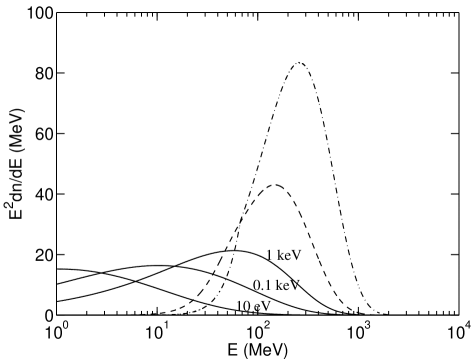
FIG. 2.: Initial spectra of photons and electrons from pion decay, for an exponential pion spectrum with the mean energy 329 MeV. The dot-dashed line shows the photon spectrum from the decay of a neutral pion. The dashed line shows the electron spectrum from the decay of a charged pion. The electrons transfer their energy to background photons through inverse Compton scattering. The resulting photon spectra at temperatures 1 keV, 100 eV and 10 eV are shown by solid lines.

F Spallation of ${}^{4}{\rm He}$ by energetic neutrons

The average energy of a nucleon produced in $\bar{\rm p}{}^{4}{\rm He}$ annihilation is $\approx 70$ MeV. This is sufficient to disintegrate a ${}^{4}{\rm He}$ nucleus. Protons and ions slow down rapidly compared to the interaction time of nuclear reactions. Neutrons thermalize much more slowly and may cause significant spallation of ${}^{4}{\rm He}$.

Destruction of even a small fraction of ${}^{4}{\rm He}$ may produce ${}^{3}{\rm He}$ or D in amounts comparable to the total abundance of these elements, but destruction of other elements is significant only if a large fraction of the nuclei is destroyed. Thus only ${\rm n}{}^{4}{\rm He}$ spallation is important.

For $T<100$ eV the neutron mean time before spallation becomes larger than the neutron lifetime and spallation gradually ceases.

G Lithium

We do not expect any drastic effects on the ${}^{7}{\rm Li}$ yield from antimatter regions. For small scales and large antimatter fractions the reduction in the ${}^{4}{\rm He}$ and ${}^{3}{\rm He}$ yields cause an even steeper reduction in the ${}^{7}{\rm Li}$ yield, but the ${}^{4}{\rm He}$ yield is a more sensitive constraint.

For large scales, annihilation and photodisintegration of ${}^{7}{\rm Li}$ is a small effect, just as for ${\rm D}$ and ${}^{3}{\rm He}$, compared to the large ${}^{3}{\rm He}$ production from ${}^{4}{\rm He}$ annihilation and photodisintegration.

Since the standard BBN (SBBN) ${}^{6}{\rm Li}$ yield is much below the ${}^{7}{\rm Li}$ yield, ${}^{6}{\rm Li}$ production from ${}^{7}{\rm Li}$ annihilation, spallation, and photodisintegration could cause a large relative increase in the ${}^{6}{\rm Li}$ yield.

The ${}^{3}{\rm H}$ and ${}^{3}{\rm He}$ from photodisintegration and annihilation have large energies. They may react with ${}^{4}{\rm He}$ to produce ${}^{6}{\rm Li}$ and ${}^{7}{\rm Li}$ before thermalizing. This nonthermal nucleosynthesis may proceed via ${}^{3}{\rm H}({}^{3}{\rm He})+{}^{4}{\rm He}\rightarrow{}^{6}{\rm Li}+{\rm n}({\rm p})$, which has a threshold of 4.80 MeV (4.03 MeV) and is therefore not available for thermal nucleosynthesis, and it may result in a ${}^{6}{\rm Li}$ yield much larger than in SBBN[53].

III Numerical Implementation

A General

We use a spherically symmetric geometry where a spherical antimatter region is surrounded by a thick shell of matter. We assume equal initial densities $n_{b}=n_{\bar{b}}$ in both regions, such that the average net baryon density ${\langle n_{B}\rangle}$ corresponds to $\langle\eta\rangle=6\times 10^{-10}$.

We give our results as a function of two parameters, the radius of the antimatter region $r_{A}$, and the antimatter-matter ratio $R$. These parameters together with the net baryon density determine the initial local baryon density $n_{b}$ and the volume fraction $f_{V}$ covered by antimatter. The volume fraction depends only on the antimatter-matter ratio

$$R=\frac{f_{V}n_{\bar{b}}}{(1-f_{V})n_{b}}=\frac{f_{V}}{1-f_{V}}.$$ (35)

The initial baryon density $n_{b}$ is linked to the volume fraction through

$${\langle n_{B}\rangle}=(1-f_{V})n_{b}-f_{V}n_{b}.$$ (36)

The radius of our grid is $L=r_{A}/f_{V}^{1/3}$. We assume reflective boundary conditions at the outer boundary of the matter shell. This models the situation where antimatter regions of radius $r_{A}$ are separated from each other by the distance $2L$ between their centers.

For $R\ll 1$, also $f_{V}\ll 1$ and $r_{A}\ll L$, so that we have a relatively small antimatter region surrounded by a much larger volume of matter.

The annihilation creates a narrow depletion zone around the boundary between the matter and antimatter regions. An accurate treatment requires a dense grid spacing in this region. The position of the boundary moves with time. Therefore a fixed non-uniform grid is not adequate. We use a steeply non-uniform grid, which is updated at every time step. The number of grid cells per unit distance is proportional to the gradient in baryon density. The total number of cells is kept constant.

We include nucleosynthesis both in matter and antimatter. In matter we follow the reactions up to $A=7$, in antimatter up to $\bar{A}=4$. Our code includes 15 isotopes: n, p, D, ${}^{3}{\rm H}$, ${}^{3}{\rm He}$, ${}^{4}{\rm He}$, ${}^{6}{\rm Li}$, ${}^{7}{\rm Li}$, ${}^{7}{\rm Be}$, $\bar{\rm n}$, $\bar{\rm p}$, $\overline{\rm D}$, ${}^{3}\overline{\rm H}$, ${}^{3}\overline{\rm He}$, and ${}^{4}\overline{\rm He}$. Heavier matter isotopes are included as sinks.

B Annihilation and diffusion

Because of the large uncertainty or lack of data for most of the relevant annihilation reactions we simply use

$$\langle\sigma v\rangle=\sigma_{0}$$ (37)

for the $\bar{\rm n}{\rm n}$, $\bar{\rm n}{\rm p}$, ${\rm n}\bar{\rm p}$, and all $\bar{\rm n}{\rm A}$, ${\rm n}\bar{\rm A}$ annihilation cross sections and

$$\langle\sigma v\rangle=C(v)\sigma_{0}$$ (38)

for $\bar{\rm p}{\rm p}$ and all $\bar{\rm p}{\rm A}$, ${\rm p}\bar{\rm A}$, and $\bar{\rm A}{\rm A}$ annihilations. Here

$$C(v)=\frac{2\pi|Z_{1}Z_{2}|\alpha/v}{1-\exp(-2\pi|Z_{1}Z_{2}|\alpha/v)},$$ (39)

and we use $\sigma_{0}=40$ mb. The velocity $v$ in the Coulomb factor $C(v)$ is the relative velocity, for which we use the thermal velocity $v=\sqrt{3T/\mu}$, where $\mu$ is the reduced mass of the annihilating pair. We also studied the effect of including an $A^{2/3}$ dependence in $\sigma_{0}$.

We assume that $\bar{\rm n}{\rm A}$ and $\bar{\rm p}{\rm A}$ have the same nuclear yields, and that ${\rm n}\bar{\rm A}$ and ${\rm p}\bar{\rm A}$ have the corresponding antiyields. The most important $\bar{\rm p}{\rm A}$ reaction is $\bar{\rm p}{}^{4}{\rm He}$. For its yield we use

$$\bar{\rm p}+{}^{4}{\rm He}\rightarrow 0.490{\rm n} + 0.309{\rm p}+0.130{\rm D}$$ (40)

$$+ 0.437{}^{3}{\rm H}+0.210{}^{3}{\rm He},$$ (41)

where we have taken the ${\rm D}$, ${}^{3}{\rm H}$, ${}^{3}{\rm He}$ yields from[37], $\sigma(\bar{\rm p}{\rm n})/\sigma(\bar{\rm p}{\rm p})=0.42$ from[40], and we assumed charge exchange has no net effect, to get the ${\rm n}$ and ${\rm p}$ yields. The $\bar{\rm n}{\rm A}$, $\bar{\rm p}{\rm A}$, ${\rm n}\bar{\rm A}$, and ${\rm p}\bar{\rm A}$ yields for other nuclei than ${\rm A}={}^{4}{\rm He}$ are not important. We estimated yields for them by assuming that $\bar{\rm p}(\bar{\rm n})$ annihilation is twice as likely with ${\rm p}$ than with ${\rm n}$ in the nucleus[41, 40], using the experimental ${\rm p}$, ${\rm D}$, and ${}^{3}{\rm H}$ yields for $\bar{\rm p}{}^{6}{\rm Li}$ and $\bar{\rm p}{}^{7}{\rm Li}$[39], and otherwise trying to mimic the $\bar{\rm p}{}^{4}{\rm He}$ data.

There is no data on annihilation of an antinucleus on a nucleus. For simplicity we assume that the lighter nucleus is annihilated completely, and the remnants of the heavier nucleus go into ${}^{4}{\rm He}$ nuclei and nucleons, with equal number of protons and neutrons. Especially, annihilation of a nucleus on an antinucleus with equal mass number leads to total annihilation.

Annihilation, nuclear reactions, and diffusion are solved together for better accuracy. Hydrodynamic expansion, spreading of the annihilation yields, and photodisintegration are treated as separate steps. We include diffusion of all ions and neutrons.

Annihilation reactions are represented by the differential equation

$$\frac{dY_{k}}{dt}=-\sum_{l}{\langle n_{B}\rangle}\langle\sigma_{kl}^{\rm ann}v\rangle Y_{k}Y_{l}=-\sum_{l}G_{kl}Y_{k}Y_{l},$$ (42)

where the indices $k$ and $l$ refer to the annihilating isotopes and $Y_{k}=n_{k}/{\langle n_{B}\rangle}$ is the relative abundance.

We integrate Eq. (42) over the time step $\Delta t$. We take the implicit equation

$$Y_{k}^{i}-Y_{k}^{i0}=-\sum_{l}G_{kl}^{i}Y_{k}^{i}Y_{l}^{i}\Delta t,$$ (43)

and linearize it into

$$Y_{k}^{i}-Y_{k}^{i0}=-\sum_{l}\mu^{i}G_{kl}^{i}(\hat{Y}_{k}^{i}Y_{l}^{i}+Y_{k}^{i}\hat{Y}_{l}^{i}-\hat{Y}_{k}^{i}\hat{Y}_{l}^{i})\Delta t.$$ (44)

Here $Y_{k}^{i0}$ is the initial abundance and $\hat{Y}$ is the solution from the previous iteration step.

We solve this equation iteratively by a modified Newton-Raphson method. The ordinary Newton-Raphson method (e.g., [54]) does not work in this case, since it often converges to an unphysical solution with negative $Y$. We stabilize the algorithm by introducing a parameter $\mu$ which initially is set to zero. We gradually increase the value of $\mu$ between iteration steps, until the solution has converged and $\mu=1$.

In our code the hydrodynamic expansion is started at a constant temperature $T=30$ keV. The results are insensitive to the starting temperature, because late times dominate the expansion. Equation (3) is solved for $n_{B}$ as an ordinary diffusion equation. The grid cells are then expanded so that the baryon distribution corresponds to the solution.

Hydrodynamic expansion is not combined into the same matrix equation with diffusion and nuclear reactions, but is treated as a separate step. For this reason the convergence of the code requires a very small time step at late times, when the hydrodynamic expansion becomes important. This limited our ability to calculate with very large scales. For our largest scale $r_{A}=10^{11}$ m, we did not get a converged result for the CMB distortion, since it is sensitive to the lowest annihilation temperatures, although our results for the nuclear abundances did converge.

C Spreading of the annihilation products and their reactions

We model the energy spectrum of a nucleus created in annihilation by an exponential distribution $\exp(-E/E_{0})/E_{0}$. The spectrum is cut off at $E=10E_{0}$. The mean kinetic energy $E_{0}$ corresponds to momentum $P_{0}=350$ MeV$/c$ for neutrons and protons, and to $P_{0}=200$ MeV$/c$ for nuclei with $A>1$.

Consider the spreading of nuclei produced during one time step, along a linear path. The spherical symmetry allows us to identify paths with same tangential distance $r_{0}$ from the symmetry center. Let $F(E,s,r_{0})dr_{0}$ denote the cumulative spectrum of nuclei at distance $s$ from the tangent point. The energy spectrum obeys the differential equation

$$F(E,s,r_{0})dr_{0} = F(E-\frac{dE}{ds}ds,s-ds,r_{0})dr_{0}$$ (46)

$$+F_{0}(E)g(r)4\pi r^{2}dr\frac{d\Omega}{4\pi}.$$

Here $g(r)$ is the number of particles created per unit volume at distance $r$ from the center, $F_{0}(E)$ is their initial spectrum, and solid angle $\Omega(r_{0})=2\pi\sqrt{1-(r_{0}/r)^{2}}$ picks directions which correspond to the tangential distance $r_{0}$.

We integrate Eq. (46) assuming a reflective boundary condition at the outer edge of the grid. Nuclei which fall below $E_{\rm min}\sim T$ are considered thermalized. The formulae for the energy loss $dE/ds$ due to various scattering processes were given in Sec. II.

Ions lose energy through Coulomb scattering on electrons and ions, and Thomson scattering on photons. Neutrons lose energy through scattering on electrons and ions, or they decay and thermalize as protons. We include all these effects. Neutrons are allowed to scatter on an ion once, after which they are stopped. The strong and weak interaction neutron reactions included are listed in Table I.

Reaction	Ref.
n+p total	[55, 56]
n+$\bar{\rm p}$ total	[57]
n+${}^{4}{\rm He}$ total	[58]
n+${}^{4}{\rm He}\rightarrow{}^{3}{\rm H}+{\rm D}$	[59] (from inverse reaction), [60]
n+${}^{4}{\rm He}\rightarrow{}^{3}{\rm H}+{\rm p}+{\rm n}$	[60]
n+${}^{4}{\rm He}\rightarrow{\rm D}+{\rm p}+2{\rm n}$	[60]
n+${}^{4}{\rm He}\rightarrow 2{\rm D}+{\rm n}$	[60]
n+${}^{4}{\rm He}\rightarrow{}^{3}{\rm He}+2{\rm n}$	[60]
n $\rightarrow$ p	$\tau$ = 886.7 s

TABLE I.: Neutron reactions and references to their cross section data.

D Nonthermal nuclear reactions

We ignore spallation of nuclei by energetic nucleons for other nuclei than ${}^{4}{\rm He}$. Our results show that even ${}^{4}{\rm He}$ spallation is a relatively small effect, which confirms that spallation of other nuclei can be safely ignored.

We ignore in this work also the production of ${}^{6}{\rm Li}$ by non-thermal ${}^{3}{\rm He}({}^{3}{\rm H})+{}^{4}{\rm He}$ reactions[53], but we are incorporating it for future work[61].

E CMB distortion

We calculate the ratio of injected energy to the CMB energy as

$$W=\int^{\rm 2keV}\frac{1}{\rho_{\rm CMB}(T)}\frac{d\bar{\rho}_{\rm ann}}{dT}dT$$ (47)

and require $W<6\times 10^{-5}$ to satisfy the CMB constraint. Here $\rho_{\rm CMB}$ is the energy density of the background radiation and $\bar{\rho}_{\rm ann}$ is the energy density released in annihilation reactions in form of photons and electrons, averaged over space. Effectively, we are assuming complete thermalization above $T=2$ keV (redshift $z\approx 8.5\times 10^{6}$) and no thermalization below it. We count into $\bar{\rho}_{\rm ann}$ half of the total annihilation energy. The other half disappears as neutrinos, and has no effect on nucleosynthesis or CMB.

F Photodisintegration

We compute the initial spectra of electrons and photons from pion decay following Sec. IIE. We assume an exponential kinetic energy distribution for the pions, with mean total energy equal to $2m_{p}/5.7$ = 329 MeV. The electrons transfer their energy to background photons through inverse Compton scattering. We compute the spectrum of the upscattered photons using the Klein-Nishina cross section, assuming a thermal background spectrum and $E_{e}\gg m_{e}$. We then redistribute the energy of the initial photons (upscattered and from $\pi_{0}$ decay), whose energies are above $E_{c}$ into the standard cascade spectrum [Eq. (21)].

The photons in this resulting spectrum have then an opportunity to photodisintegrate. These photons may pair produce on a nucleus, Compton scatter, or photodisintegrate nuclei. We allow an unlimited number of Compton scatterings for a single photon, but we remove the photon after the production of an e^± pair or a photodisintegration reaction. The created e^± pairs, as well as the background electrons which gain energy in Compton scattering, will produce a second generation of non-thermal photons by inverse Compton scattering. These secondary photons are, however, much less energetic than the primary ones, and we ignore them.

The photodisintegration reactions included in our code are listed in Table II.

In [26] we used the results of Protheroe, Stanev and Berezinsky (PSB)[48] for photodisintegration. PSB calculated the amount of ${}^{3}{\rm He}$ and D produced per 1 GeV of energy released in the form of photons and electrons, as a function of redshift. However, their result does not apply for annihilation at low temperatures, when a significant part of the initial photon spectrum from annihilation is below the threshold for photon-photon pair production. In Fig. 3 we compare the PSB yields with the more detailed treatment described above which we are now using.

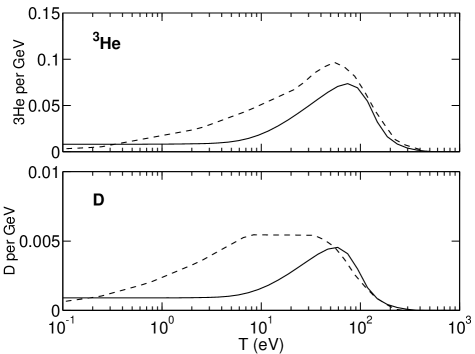
FIG. 3.: Comparison of our photodisintegration ${}^{3}{\rm He}$ and D yields (solid lines) with Protheroe et al.[48] (dashed lines).

We get less ${}^{3}{\rm He}$ (${\rm D}$) than the PSB yield for $T<100\mbox{ eV}$ ($50\mbox{ eV}$). There are two reasons for this difference.

Reaction	Ref.
D+$\gamma\rightarrow$ p+n	[55] (from inverse reaction)
${}^{3}{\rm H}+\gamma\rightarrow$ D+n	[62, 63]
${}^{3}{\rm H}+\gamma\rightarrow$ p+2n	[62]
${}^{3}{\rm He}+\gamma\rightarrow$ D+p	[64]
${}^{3}{\rm He}+\gamma\rightarrow$ 2p+n	[62]
${}^{4}{\rm He}+\gamma\rightarrow{}^{3}{\rm He}$+n	[65]
${}^{4}{\rm He}+\gamma\rightarrow{}^{3}{\rm H}$+p	same as ${}^{4}{\rm He}+\gamma\rightarrow{}^{3}{\rm He}$+n
${}^{4}{\rm He}+\gamma\rightarrow$ D+p+n	[66]

TABLE II.: Photodisintegration reactions and references to their cross section data.

First, our cross sections (Table II) differ somewhat from what PSB used. The main difference is for large photon energies $E_{\gamma}\gtrsim 200\mbox{ MeV}$, where the ${}^{4}{\rm He}$ photodisintegration cross section again becomes large and a pion is produced (“pion photoproduction”). PSB assumed large ${\rm D}$ and ${}^{3}{\rm He}$ yields for these reactions. Available data[67] gives very small cross sections for the ${}^{4}{\rm He}+\gamma\rightarrow{}^{3}{\rm H}+{\rm p}$, ${}^{4}{\rm He}+\gamma\rightarrow{\rm D}+{\rm p}+{\rm n}$, and ${}^{4}{\rm He}+\gamma\rightarrow{\rm D}+{\rm D}$ channels for $E_{\gamma}>200\mbox{ MeV}$. Accordingly, we set the ${\rm D}$ and ${}^{3}{\rm He}$ yields to zero in this range. Therefore we get lower ${\rm D}$ and ${}^{3}{\rm He}$ production at low temperatures as the cascade moves to these higher energies.

Second, for low temperatures the cascade energies move up to and beyond the energies of the initial annihilation photons. Since we only convert to the cascade those initial photons whose energy is above the cascade turnover $E_{c}$, our photon spectrum for photodisintegration does not move up further. Therefore the ${\rm D}$ and ${}^{3}{\rm He}$ yields become almost independent of temperature for $T<5\mbox{ eV}$. In our nucleosynthesis runs most of the annihilation takes place for $T>5\mbox{ eV}$, but for antimatter regions larger than $r_{A}\sim 10^{11}$ m annihilation occurs at these lower temperatures and the photodisintegration contribution should become independent of $r_{A}$.

IV Results

We show light element yields as a function of the radius $r_{A}$ of the antimatter region and the antimatter-matter ratio $R$ in Figs. 4, 5, and 6. We show also the temperature around which the annihilation is taking place. All results are for a net baryon density $\langle\eta\rangle=6\times 10^{-10}$.

For scales smaller than $r_{A}=10^{5}$ m, annihilation happens before the weak freeze-out, and has no effect on BBN. For scales between $r_{A}=10^{5}$ m and $r_{A}=10^{8}$ m, neutron annihilation before ${}^{4}{\rm He}$ formation leads to a reduction in the ${}^{4}{\rm He}$ yield compared to standard BBN (SBBN).

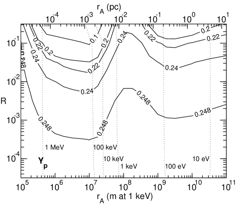
FIG. 4.: The yield of ${}^{4}{\rm He}$ as a function of the antimatter-matter ratio $R$ and the radius $r_{A}$ of the antimatter regions. The SBBN result, which is approached in the lower left corner, is $Y_{p}=0.2484$. The dotted lines show contours of $T_{\rm ann}$, the temperature at which half of the antimatter has annihilated.

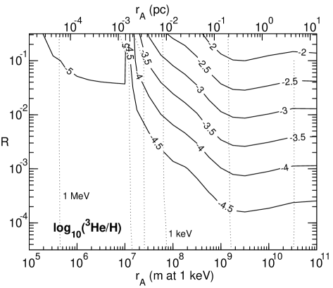
FIG. 5.: Same as Fig. 4, but for ${}^{3}{\rm He}$. The SBBN yield is ${}^{3}{\rm He}/{\rm H}=1.06\times 10^{-5}$.

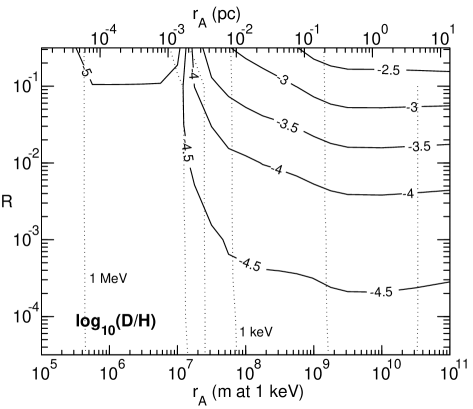
FIG. 6.: Same as Fig. 4, but for ${\rm D}$. The SBBN yield is ${\rm D}/{\rm H}=2.70\times 10^{-5}$.

If annihilation is not complete before ${}^{4}{\rm He}$ formation, it is delayed significantly because the neutrons have disappeared and ion diffusion is much slower than neutron diffusion. There will then be a second stage of annihilation well after nucleosynthesis, at $T\sim 3$ keV or below. This leads to a substantial increase in the yields of ${}^{3}{\rm He}$ and D.

Antimatter regions in the size range $r_{A}\sim 10^{7}$–$10^{8}$ m are annihilated in two stages. In the lower part of this range, practically all antineutrons diffuse out of the antimatter region and are annihilated in the first stage, but neutrons diffusing towards the antimatter region manage to annihilate only an outer layer of the antiprotons before nucleosynthesis swallows the remaining neutrons. Thus the antimatter region that is left for the second stage of annihilation consists of antiprotons only.

Larger antimatter regions, $r_{A}\gtrsim 4\times 10^{7}$ m, have also antineutrons left by the time of nucleosynthesis, and thus antinucleosynthesis, producing mainly ${}^{4}\overline{\rm He}$, takes place in the antimatter region. The main significance of this is that ${\rm p}{}^{4}\overline{\rm He}$ annihilation will later produce high-energy antinucleons, which penetrate deep into the matter region before annihilating. Thus not all of the annihilation occurs in the annihilation zone (“primary” annihilation), but there is also a significant amount of “secondary” annihilation occurring in a large volume surrounding the annihilation zone.

The main annihilation reaction during the second stage is $\bar{\rm p}{}^{4}{\rm He}$. It produces ${}^{3}{\rm He}$ and a smaller amount of D. Because of their high energy, these annihilation products penetrate some distance away from the annihilation zone. Less than half of them end up in the antimatter region and are annihilated immediately. The rest end up in the matter region, but partly so close to the antimatter region that they are sucked into the annihilation zone and annihilated later (except for the largest scales studied).

For $r_{A}\gtrsim 5\times 10^{7}$ m, part of the annihilation occurs below $T=0.6\mbox{ keV}$ where ${}^{4}{\rm He}$ photodisintegration produces ${}^{3}{\rm He}$ and D.

Thus there are two main contributions to ${}^{3}{\rm He}$ and D production: annihilation and photodisintegration. We show these contributions separately in Figs. 7 and 8.

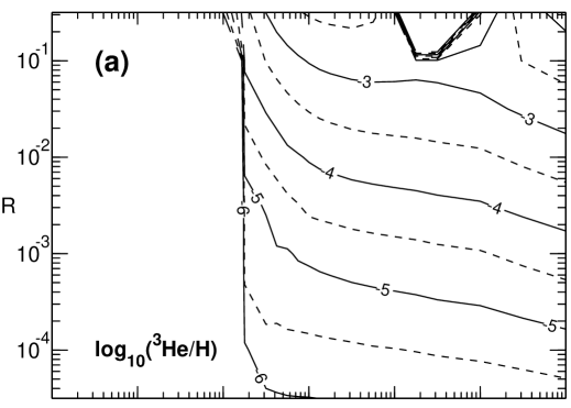
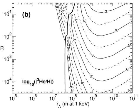
FIG. 7.: Contribution to the ${}^{3}{\rm He}$ yield from a) annihilation and b) photodisintegration. To the left of the thick line in (b) the contribution is negative, since ${}^{3}{\rm He}$ photodisintegration dominates over photoproduction.

Figure 7a shows the net production of ${}^{3}{\rm He}$ (including ${}^{3}{\rm H}$) from all annihilation reactions. The most important ${}^{3}{\rm He}$ producing reaction is $\bar{\rm p}{}^{4}{\rm He}$. Another is $\bar{\rm n}{}^{4}{\rm He}$, where the antineutrons come from ${\rm p}{}^{4}\overline{\rm He}$ annihilation. ${}^{3}{\rm He}$ is destroyed primarily by $\bar{\rm p}{}^{3}{\rm He}$ annihilation in the annihilation zone.

Annihilation production of ${}^{3}{\rm He}$ increases steeply from $r_{A}=2\times 10^{7}$ m to $5\times 10^{7}$ m as a larger part of the antimatter region survives till the second stage. For $r_{A}>5\times 10^{7}$ m, the annihilation production of ${}^{3}{\rm He}$ keeps increasing with scale, since the annihilation shifts to lower temperatures where the ${}^{3}{\rm He}$ produced in annihilation travels longer (comoving) distances, and is thus able to better survive annihilation.

${}^{3}{\rm He}$ produced in the matter region by the secondary annihilation is much more likely to survive and thus this secondary annihilation produces more, or at least a comparable amount of, surviving ${}^{3}{\rm He}$ than the primary annihilation in the range $r_{A}\sim 10^{8}$–$5\times 10^{9}$ m, where most of the ${}^{3}{\rm He}$ from primary annihilation gets annihilated. In [26] we did not include this secondary annihilation, and therefore we got a smaller annihilation contribution.

Figure 7b shows the net production of ${}^{3}{\rm He}$ from all photodisintegration reactions. Photodisintegration of ${}^{3}{\rm He}$ sets in for $r_{A}\gtrsim 2\times 10^{7}$ m but has only a small effect. For $r_{A}>5\times 10^{7}$ m, photoproduction of ${}^{3}{\rm He}$ from ${}^{4}{\rm He}$ overcomes ${}^{3}{\rm He}$ photodestruction and increases up to $r\sim 10^{9}$ m, as a larger part of the cascade exceeds the ${}^{4}{\rm He}$ photodisintegration threshold.

For $r_{A}\gtrsim 10^{10}$ m, photoproduction of ${}^{3}{\rm He}$ decreases again, as the cascade keeps moving to higher energies. The photodisintegration cross sections for ${}^{3}{\rm He}$ and D production are smaller at these higher energies, and because the individual photons have higher energies there are fewer of them. For even larger scales, $r_{A}>10^{11}$ m, we would expect the photoproduction to stabilize as the cascade gets replaced by the initial annihilation spectrum (cf. Fig. 3).

The different dependence of these two contributions on $T$, and thus on $r_{A}$, means that annihilation production dominates for $r_{A}=2\times 10^{7}$–$5\times 10^{8}$ m ($T_{\rm ann}>250\mbox{ eV}$) and $r_{A}>3\times 10^{10}$ m ($T_{\rm ann}<10\mbox{ eV}$), but photoproduction dominates in the intermediate range $r_{A}=5\times 10^{8}$– $3\times 10^{10}$ m.

In Fig. 7a, the feature at $R>0.1$, $r_{A}=10^{9}$–$10^{10}$ m is due to annihilation of the photoproduced ${}^{3}{\rm He}$.

For ${\rm D}$ (see Fig. 8) we observe the same effects, with some differences. Annihilation produces about 5 times more ${}^{3}{\rm He}$ than ${\rm D}$, but ${\rm D}$ penetrates farther from the annihilation zone and thus survives better. Therefore the ${\rm D}$ yield from annihilation is less dependent on $r_{A}$, as most of the ${\rm D}$ survives already for smaller scales. The ratio of the net annihilation production of ${}^{3}{\rm He}$ and ${\rm D}$ is therefore less than 5, and approaches this number only for the largest scales, where finally most of the ${}^{3}{\rm He}$ also survives.

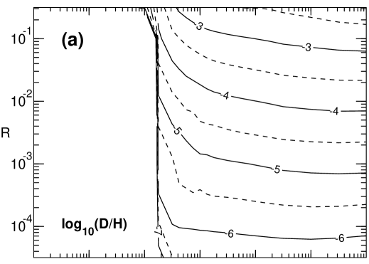
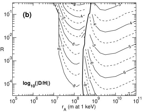
FIG. 8.: Same as Fig. 7, but for the ${\rm D}$ yield.

Photodisintegration of ${\rm D}$ begins already at $T=5.3\mbox{ keV}$, so it occurs always when the second annihilation stage is reached. Photoproduction of ${\rm D}$ from ${}^{4}{\rm He}$ can only begin at $T=0.45\mbox{ keV}$. Also the ${\rm D}$ yield from ${}^{4}{\rm He}$ photodisintegration is less than a tenth of the ${}^{3}{\rm He}$ yield. Therefore ${\rm D}$ photoproduction overcomes photodisintegration only for scales $r_{A}\gtrsim 3\times 10^{8}$ m.

The third significant mechanism for ${\rm D}$ and ${}^{3}{\rm He}$ production caused by annihilation is spallation of ${}^{4}{\rm He}$ by the high-energy neutrons from $\bar{\rm p}{}^{4}{\rm He}$ annihilation. For the scales $r_{A}=10^{7}$–$10^{8}$ m its ${\rm D}$ and ${}^{3}{\rm He}$ yields are about 10% of that by annihilation reactions. For larger scales its relative importance falls off, as neutrons decay into protons, which are then thermalized, before encountering a ${}^{4}{\rm He}$ nucleus.

Because of the large uncertainty about the annihilation cross sections in reactions involving other nuclei than just nucleons, we studied the effect of including an $A^{2/3}$ dependence in the cross section. This did not have a significant effect on the primary annihilation in the annihilation zone, but increasing the $\bar{\rm n}{}^{4}{\rm He}$ cross section increased the probability of secondary antineutrons annihilating ${}^{4}{\rm He}$ instead of protons. Thus we got an increased ${}^{3}{\rm He}$ yield for distance scales $r_{A}\sim 10^{8}$–$5\times 10^{9}$ m. Reducing the $\bar{\rm n}{}^{4}{\rm He}$ cross section would have an opposite effect.

Comparing our calculated yields to the observed abundances and the primordial abundances derived from them[68, 69], we obtain upper limits to the amount of antimatter in the early universe. We plot the limits from BBN and CMB on the antimatter-matter ratio $R$ as a function of the radius of the antimatter region in Fig. 9.

For small antimatter regions the limit comes from underproduction of ${}^{4}{\rm He}$. Using $Y_{p}=0.22$ as our lower limit to the primordial ${}^{4}{\rm He}$ mass fraction, we obtain an upper limit $R\lesssim 0.02$–0.04 for $r_{A}=0.6$–$20\times 10^{6}$ m. Because this result is obtained from a calculation with the net baryon density $\langle\eta\rangle=6\times 10^{-10}$, corresponding to the SBBN yield $Y_{p}=0.248$, a better way to state our ${}^{4}{\rm He}$ constraint is that we allow a maximum reduction of $\Delta Y_{p}=0.028$ from the SBBN result. Different assumptions on $\eta$ and observed $Y_{p}$ could give a smaller acceptable $\Delta Y_{p}$ and thus a tighter limit on $R$. But this does not work in the other direction, since the ${}^{4}{\rm He}$ yield falls very rapidly with increasing $R$. Thus the limit on $R$ can hardly be relaxed from our stated value by using different observational constraints.

At larger scales, $r_{A}>2\times 10^{7}$ m, the limit is set by overproduction of ${}^{3}{\rm He}$. There has been much uncertainty in the estimated primordial ${}^{3}{\rm He}$ abundance, because of a large scatter in its observed abundances and uncertainties about its chemical evolution[68, 70]. Current knowledge suggests a probable primordial abundance of ${}^{3}{\rm He}/{\rm H}\sim 10^{-5}$, with three times this value a reasonable upper limit[70]. Thus we have used the constraint ${}^{3}{\rm He}/{\rm H}<10^{-4.5}$.

The upper limit to $R$ from ${}^{3}{\rm He}$ falls rapidly as the distance scale is increased from $2\times 10^{7}$ m to $10^{9}$ m, where the limit becomes $R\lesssim 2\times 10^{-4}$. For even larger scales the limit is slightly relaxed but stays below $3\times 10^{-4}$.

Fig. 9 can be compared to Fig. 2 of Rehm and Jedamzik[25] or to Fig. 2 of [26]. Our ${}^{4}{\rm He}$ yield is slightly larger and the corresponding limit to $R$ weaker than in [25], because our net baryon density, $\langle\eta\rangle=6\times 10^{-10}$, is larger than the one used in [25], $\langle\eta\rangle=3.43\times 10^{-10}$. Near $r_{A}\sim 10^{8}$ m we now get a tighter limit on $R$ due to a higher ${}^{3}{\rm He}$ yield than we gave in [26]. This is due to ${}^{3}{\rm He}$ production by secondary annihilation in the matter region, which was ignored in [26].

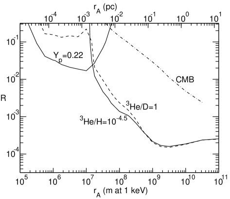
FIG. 9.: Upper limits from BBN and CMB to the antimatter-matter ratio $R$ as a function of the radius $r_{A}$ of the antimatter regions. The area above the solid lines is excluded by ${}^{4}{\rm He}$ underproduction ($Y_{p}<0.22$) or ${}^{3}{\rm He}$ overproduction (${}^{3}{\rm He}/{\rm H}>10^{-4.5}$). The dashed line gives an alternative limit from using ${}^{3}{\rm He}/{\rm D}>1$ as the criterion for ${}^{3}{\rm He}$ overproduction. The dot-dashed line is the limit from CMB distortion.

These limits are stronger than those from the CMB spectrum distortion for scales $r_{A}\leq 10^{11}$ m. We did not calculate the yields for larger scales, but the ${}^{3}{\rm He}$ and ${\rm D}$ yields should become roughly independent of $r_{A}$, since for these larger scales the primary annihilation products penetrate far enough from the annihilation region to survive, and the spectrum responsible for photodisintegration is the initial annihilation spectrum, so the dependence on the annihilation temperature disappears. The CMB limit should then become stronger than the ${}^{3}{\rm He}$ constraint near the scale $r_{A}\sim 10^{12}$ m.

V Conclusions

We have studied the effect of antimatter regions of a comoving size $r_{A}\sim 10^{-5}$–$10$ pc on big bang nucleosynthesis. Smaller antimatter regions annihilate before weak freeze-out and are not likely to lead to observable consequences. Larger regions annihilate close to, or after recombination, and the amount of antimatter in such regions is tightly constrained by the CMB and CDG spectra.

Regions smaller than $r_{A}\sim 2\times 10^{-3}$ pc annihilate before nucleosynthesis. The annihilation occurs due to neutron and antineutron diffusion and leads to a reduction in the $n/p$ ratio and thus to a reduction in $Y_{p}$. Requiring $Y_{p}\geq 0.22$, we obtain an upper limit $R\lesssim$ few % for the primordial antimatter-matter ratio for antimatter regions in the size range $r_{A}\sim(0.1$–$2)\times 10^{-3}$ pc.

If the annihilation is not complete by nucleosynthesis, at $T\sim 80$ keV, it is significantly delayed, since all neutrons and antineutrons are incorporated into ${}^{4}{\rm He}$ and ${}^{4}\overline{\rm He}$, and (anti)proton diffusion is much slower. There will be a second stage of annihilation at $T\lesssim 3$ keV, when proton and ion diffusion finally become effective in mixing the remaining antimatter with matter.

This second stage of annihilation leads to production of a large amount of ${}^{3}{\rm He}$ and a smaller amount of D, through several mechanisms.

Annihilation of ${}^{4}{\rm He}$ with antiprotons in the annihilation zone separating the matter and antimatter region produces ${}^{3}{\rm He}$ and ${\rm D}$ which are deposited some distance away from the annihilation zone. A large fraction of these annihilation products gets however sucked into the annihilation zone later and is thus annihilated. The surviving fraction increases with increasing distance scale, since this corresponds to a decreasing annihilation temperature. At lower temperatures the energetic ions from annihilation penetrate larger (comoving) distances into the matter region.

Antinucleosynthesis in the antimatter region produces ${}^{4}\overline{\rm He}$, whose annihilation produces antinucleons and smaller antinuclei. Of these, especially the antineutrons penetrate deep into the matter region, where they can annihilate ${}^{4}{\rm He}$ producing ${}^{3}{\rm He}$, which has now a much better chance to survive.

An important source of ${}^{3}{\rm He}$ and D is photodisintegration of ${}^{4}{\rm He}$ by the annihilation radiation. The large energy part of the initial radiation spectrum is converted into an electromagnetic cascade spectrum. The large-energy cut-off of the cascade exceeds the ${}^{4}{\rm He}$ photodisintegration threshold when the temperature has fallen below 0.6 keV. For $r_{A}\gtrsim 3\times 10^{-2}$ pc most of the annihilation occurs below this temperature and thus the photoproduction of ${}^{3}{\rm He}$ and D becomes important. Photodisintegration of ${}^{4}{\rm He}$ is the dominant source of ${}^{3}{\rm He}$ for $r_{A}\sim$ 0.1–10 pc. For larger distance scales the annihilation mainly occurs at lower temperatures where the photon spectrum shifts to higher energies where it causes less photodisintegration.

Another source of ${}^{3}{\rm He}$ and D is the spallation of ${}^{4}{\rm He}$ by high-energy neutrons from annihilation reactions. This effect is at least an order of magnitude smaller than the ones discussed above.

${}^{3}{\rm He}$ and D are also destroyed by photodisintegration, but since the total amount of these isotopes is much less than that of ${}^{4}{\rm He}$, this is a small effect.

For scales larger than $r_{A}\sim 2\times 10^{-3}$ pc the tightest constraint on the primordial amount of antimatter is due to ${}^{3}{\rm He}$ overproduction. $\bar{\rm p}{}^{4}{\rm He}$ annihilation produces several times more ${}^{3}{\rm He}$ than D and ${}^{4}{\rm He}$ photodisintegration produces over 10 times more ${}^{3}{\rm He}$ than D. For scales larger than $r_{A}\sim 0.1$ pc, the requirement ${}^{3}{\rm He}/{\rm H}<10^{-4.5}$ gives an upper limit $R\lesssim 3\times 10^{-4}$.

Rehm and Jedamzik[71] have studied this same problem and obtained results that seem to be in qualitative agreement with ours, but they find a lower ${}^{3}{\rm He}$ yield. Their upper limit to $R$ from ${}^{3}{\rm He}$ overproduction is weaker than ours by about a factor of 2. They also criticize our use of ${}^{3}{\rm He}/{\rm H}$ as a constraint. Therefore we show in Fig. 9 also the constraint ${}^{3}{\rm He}/{\rm D}<1$, which is observationally more secure[50]. As can be seen from the figure, the limits to $R$ stay essentially the same. By assuming that the low ${}^{6}{\rm Li}$/H observed in some Population II and disk stars is an upper limit to its primordial value, they obtain an even tighter limit on $R$ from ${}^{6}{\rm Li}$ overproduction[71]. However, ${}^{6}{\rm Li}$ is very fragile and is thus likely to be depleted in these stars. The main source of ${}^{6}{\rm Li}$ is spallation by cosmic rays in the interstellar medium. Thus the primordial abundance of ${}^{6}{\rm Li}$ based on observations is very uncertain, as noted also in [71], and could be much lower or much higher than the one observed.

In conclusion, we have established nucleosynthesis constraints on the amount of antimatter in the early universe which are tighter, by a large factor, than those from the CMB spectrum, or any other known observational constraint, for antimatter regions smaller than $\sim 10$ pc.

REFERENCES

- [1] Electronic address: Hannu.Kurki-Suonio@helsinki.fi
- [2] Electronic address: Elina.Sihvola@helsinki.fi
- [3] G. Steigman, Ann. Rev. Astron. Astrophys. 14, 339 (1976).
- [4] A.G. Cohen, A. De Rújula, and S.L. Glashow, Astrophys. J. 495, 539 (1998).
- [5] W.H. Kinney, E.W. Kolb, and M.S. Turner, Phys. Rev. Lett. 79, 2620 (1997).
- [6] A.G. Cohen and A. De Rújula, Astrophys. J. Lett. 496, L63 (1998).
- [7] M.Yu. Khlopov, Gravitation and Cosmology, 4, 69 (1998).
- [8] S. Ahlen et al., Nucl. Instrum. Meth. A350, 351 (1994); ams.cern.ch/.
- [9] AMS Collaboration, Phys. Lett. B461, 387 (1999).
- [10] E.R. Harrison, Phys. Rev. D 167, 1170 (1968).
- [11] R. Omnès, Phys. Rev. Lett. 23, 38 (1969); Phys. Rev. D 1, 723 (1970); R. Omnès, Phys. Rep. 3, 1 (1972); J.J. Aly, S. Caser, R. Omnès, J.L. Puget, and G. Valladas, Astron. Astrophys. 35, 271 (1974).
- [12] R.W. Brown and F.W. Stecker, Phys. Rev. Lett. 43, 315 (1979); F.W. Stecker, Phys. Rev. Lett. 44, 1237 (1980); G. Senjanović and F.W. Stecker, Phys. Lett. 96B, 285 (1980); F.W. Stecker, Nucl. Phys. B252, 25 (1985); R.N. Mohapatra and G. Senjanović, Phys. Rev. D 20, 3390 (1979); Phys. Rev. Lett. 42, 1651 (1979); A. Vilenkin, Phys. Rev. D 23, 852 (1981); K. Sato, Phys. Lett. 99B, 66 (1981).
- [13] V.A. Kuzmin, M.E. Shaposhnikov, and I.I. Tkachev, Phys. Lett. 105B, 167 (1981); A.K. Mohanty and F.W. Stecker, Phys. Lett. 143B, 351 (1984).
- [14] M.V. Chizhov and A.D. Dolgov, Nucl. Phys. B372, 521 (1992).
- [15] D. Comelli, M. Pietroni, and A. Riotto, Nucl. Phys. B412, 441 (1994); G.M. Fuller, K. Jedamzik, G.J. Mathews, and A. Olinto, Phys. Lett. B333, 135 (1994).
- [16] M. Giovannini and M.E. Shaposhnikov, Phys. Rev. Lett. 80, 22 (1998); Phys. Rev. D 57, 2186 (1998).
- [17] A.D. Dolgov, Phys. Rep. 222, 309 (1992); A.D. Dolgov, hep-ph/9605280.
- [18] A. Dolgov and J. Silk, Phys. Rev. D 47, 4244 (1993).
- [19] M.Yu. Khlopov, S.G. Rubin, and A.S. Sakharov, hep-ph/0003285.
- [20] M.Yu. Khlopov, R.V. Konoplich, R. Mignani, S.G. Rubin, and A.S. Sakharov, Astropart. Phys. 12, 367 (2000).
- [21] E.L. Wright et al., Astrophys. J. 420, 450 (1994); D.J. Fixsen, E.S. Cheng, J.M. Gales, J.C. Mather, R.A. Shafer, and E.L. Wright, Astrophys. J. 473, 576 (1996).
- [22] F. Combes, O. Fassi-Fehri, and B. Leroy, Nature 253, 25 (1975); J.J. Aly, Astron. Astrophys. 64, 273 (1978).
- [23] V.M. Chechetkin, M.Yu. Khlopov, M.G. Sapozhnikov, and Ya.B. Zeldovich, Phys. Lett. 118B, 329 (1982); V.M. Chechetkin, M.Yu. Khlopov, and M.G. Sapozhnikov, Riv. Nuovo Cimento 5, 1 (1982); F. Balestra, G. Piragino, D.B. Pontecorvo, M.G. Sapozhnikov, I.V. Falomkin, and M.Yu. Khlopov, Sov. J. Nucl. Phys. 39, 626 (1984); Yu.A. Batusov et al., Nuovo Cimento Lett. 41, 223 (1984).
- [24] I. Halm, Phys. Lett. B188, 403 (1987); R. Domínguez-Tenreiro and G. Yepes, Astrophys. J. Lett. 317, L1 (1987); G. Yepes and R. Domínguez-Tenreiro, Astrophys. J. 335, 3 (1988); M.H. Reno and D. Seckel, Phys. Rev. D 37, 3441 (1988).
- [25] J.B. Rehm and K. Jedamzik, Phys. Rev. Lett. 81, 3307 (1998).
- [26] H. Kurki-Suonio and E. Sihvola, Phys. Rev. Lett. 84, 3756 (2000).
- [27] C.R. Alcock, D.S. Dearborn, G.M. Fuller, G.J. Mathews, and B.S. Meyer, Phys. Rev. Lett. 64, 2607 (1990).
- [28] K. Jedamzik and G.M. Fuller, Astrophys. J. 423, 33 (1994).
- [29] F.L. Shapiro, Zh. Eksp. Teor. Fiz. 34, 1648 (1958) [Sov. Phys. JETP 7, 1132 (1958)].
- [30] J. Carbonell, K.V. Protasov, and A. Zenoni, Phys. Lett. B397, 345 (1997).
- [31] J. Carbonell and K.V. Protasov, Hyp. Int. 76, 327 (1993).
- [32] J. Carbonell and K. Protasov, Z. Phys. A 355, 87 (1996).
- [33] A. Bianconi, G. Bonomi, M.P. Bussa, E. Lodi Rizzini, L. Venturelli, and A. Zenoni, nucl-th/0003006.
- [34] C.J. Batty, Rep. Progr. Phys. 52, 165 (1989).
- [35] J. Carbonell and K.V. Protasov, J. Phys. G 18, 1863 (1992).
- [36] K.V. Protasov, G. Bonomi, E. Lodi Rizzini, and A. Zenoni, Eur. Phys. J. A7, 429 (2000).
- [37] F. Balestra et al., Nuov. Cim. 100A, 323 (1988).
- [38] F. Balestra et al., Phys. Lett. B215, 247 (1988); F. Balestra et al., Nucl. Phys. A491, 572 (1989); D. Polster et al., Phys. Rev. C 51, 1167 (1995).
- [39] A.S. Sudov et al., Nucl. Phys. A554, 223 (1993).
- [40] F. Balestra et al., Nucl. Phys. A465, 714 (1987).
- [41] T. von Egidy, Nature 328, 773 (1987).
- [42] J.D. Jackson, Classical Electrodynamics, 2nd ed. (Wiley, New York, 1975), Chapter 13.
- [43] T.H. Stix, Plasma Phys. 14, 367 (1972).
- [44] D. Lindley, Mon. Not. R. Astron. Soc. 193, 593 (1980); Astrophys. J. 294, 1 (1985); J. Audouze, D. Lindley, and J. Silk, Astrophys. J. Lett. 293, L53 (1985); J. Ellis, D.V. Nanopoulos, and S. Sarkar, Nucl. Phys. B259, 175 (1985); E. Holtmann, M. Kawasaki, K. Kohri, and T. Moroi, Phys. Rev. D 60, 023506 (1999).
- [45] S. Dimopoulos, R. Esmailzadeh, L.J. Hall, and G.D. Starkman, Phys. Rev. Lett. 60, 7 (1988); Astrophys. J. 330, 545 (1988); Nucl. Phys. B311, 699 (1989).
- [46] R. Svensson and A.A. Zdziarski, Astrophys. J. 349, 415 (1990).
- [47] J. Ellis, G.B. Gelmini, J.L. Lopez, D.V. Nanopoulos, and S. Sarkar, Nucl. Phys. B373, 399 (1992).
- [48] R.J. Protheroe, T. Stanev, and V.S. Berezinsky, Phys. Rev. D 51, 4134 (1995).
- [49] M. Kawasaki and T. Moroi, Astrophys. J. 452, 506 (1995).
- [50] G. Sigl, K. Jedamzik, D.N. Schramm, and V.S. Berezinsky, Phys. Rev. D 52, 6682 (1995).
- [51] K.R. Lang, Astrophysical Formulae, 2nd ed. (Springer, Berlin, 1980), p. 449.
- [52] F. Halzen and A.D. Martin, Quarks & Leptons: An Introductory Course in Modern Particle Physics, (Wiley, New York, 1984), p. 263.
- [53] K. Jedamzik, Phys. Rev. Lett. 84, 3248 (2000).
- [54] W.H. Press, S.A. Teukolsky, W.T. Vetterling, and B.P. Flannery, Numerical Recipes in Fortran, 2nd ed. (Cambridge University Press, 1992).
- [55] G.M. Hale, and P.G. Young, ENDF/B-VI evaluation, material 125, revision 4 (1998).
- [56] P.W. Lisowski, R.E. Shamu, G.F. Auchampaugh, N.S.P. King, M.S. Moore, G.L. Morgan, and T.S. Singleton, Phys. Rev. Lett. 49, 255 (1982).
- [57] G.S. Mutchler et al., Phys. Rev. D 38, 742 (1988).
- [58] R.A. Nisley, G.M. Hale, and P.G. Young, ENDF/B-VI evaluation, material 228, revision 1 (1973); R.E. Shamu, G.G. Ohlsen, and P.G. Young, Phys. Lett. 4, 286 (1963); P. Hillman, R.H. Stahl, and N.F. Ramsey, Phys. Rev. 96, 115 (1954); D.F. Measday and J.N. Palmieri, Nucl. Phys. 85, 129 (1966).
- [59] H. Liskien and A. Paulsen, Nuclear Data Tables A11, 569 (1973).
- [60] P.E. Tannenwald, Phys. Rev. 89, 508 (1953).
- [61] E. Sihvola, work in progress.
- [62] D.D. Faul, B.L. Berman, P. Meyer, and D.L. Olson, Phys. Rev. C 24, 849 (1981).
- [63] D.M. Skopik, D.H. Beck, J. Asai, and J.J. Murphy II, Phys. Rev. C 24, 1791 (1981).
- [64] G. Ticcioni, S.N. Gardiner, J.L. Matthews, and R.O. Owens, Phys. Lett. 46B, 369 (1973).
- [65] J.R. Calarco, B.L. Berman, and T.W. Donnelly, Phys. Rev. C 27, 1866 (1983).
- [66] F. Balestra et al., Nuov. Cim. 38A, 145 (1977).
- [67] J. Arends, J. Eyink, A. Hegerath, H. Hartmann, B. Mecking, G. Nöldeke, and H. Rost, Phys. Lett. 62B, 411 (1976); Nucl. Phys. A322, 253 (1979); M. MacCormick et al., Phys. Rev. C 55, 1033 (1997).
- [68] B.E.J. Pagel, Nucleosynthesis and Chemical Evolution of Galaxies, (Cambridge University Press, Cambridge, 1997).
- [69] K.A. Olive and D.N. Schramm, in Particle Data Group, C. Caso et al., Eur. Phys. J. C 3, 1 (1998), p.119; K.A. Olive, G. Steigman, and T.P. Walker, astro-ph/9905320; D. Tytler, J.M. O’Meara, N. Suzuki, and D. Lubin, astro-ph/0001318.
- [70] M. Tosi, astro-ph/0001409.
- [71] J.B. Rehm and K. Jedamzik, astro-ph/0006381.