Constraints on Cold ${\rm H}_{2}$ Clouds from Gravitational Microlensing Searches.

Abstract

It has been proposed that the Galaxy might contain a population of cold clouds in numbers sufficient to account for a substantial fraction of the total mass of the Galaxy. These clouds would have masses of $\sim 10^{-3}M_{\odot}$ and sizes $\sim 10$ AU. We consider here the lensing effects of such clouds on the light from background stars. A semianalytical formalism for calculation of the magnification event rate produced by such gaseous lensing is developed, taking into account the spatial distribution of the dark matter in the Galaxy, the velocity distribution of the lensing clouds and source stars, and motion of the observer. Event rates are calculated for the case of gaseous lensing of stars in the Large Magellanic Cloud and results are directly compared with the results of the search for gravitational microlensing events undertaken by the MACHO collaboration. The MACHO experiment strongly constrains the properties of the proposed molecular clouds, but does not completely rule them out. Future monitoring programs will either detect or more strongly constrain this proposed population.

1 Introduction

The nature of the dark matter dominating the mass of the Galaxy remains elusive. Although nonbaryonic forms of dark matter are one possible explanation, it is possible that much or most of the mass may be baryonic. Recent results from gravitational microlensing experiments, such as MACHO and EROS (Alcock et al. 2000; Lasserre et al. 2000), have put severe constraints on the abundances of compact baryonic objects in the Galaxy, - such as brown dwarfs, old white dwarfs, neutron stars, or black hole remnants - thus virtually removing stellar objects as candidates for being the major constituent of the dark matter (Alcock et al. 2000; Freese, Fields, & Graff 2000; Lasserre et al. 2000).

It has recently been proposed that the dark matter in the Galaxy could consist of small, cold clouds of H₂ (Pfenniger, Combes, & Martinet 1994; De Paolis et al. 1995a, 1995b, 1996; Gerhard & Silk 1996). Walker & Wardle (1998) pointed out that such clouds could be responsible for the extreme scattering events (ESEs; Fiedler et al. 1994), which would occur when the line of sight to an extragalactic point radio source is crossed by the photoionized cloud envelope. In a later paper, Wardle & Walker (1999) considered the thermal stability of such clouds and showed that these clouds could be stable against heating by cosmic rays. These clouds could have masses of the order of Jupiter’s mass ($10^{-3}M_{\odot}$) and radii $R_{cl}\approx 10$ AU. If they exist, these clouds could also naturally explain the core radii of galaxies (Walker 1999) as well as the $\gamma$-ray emission from the Galactic halo (Kalberla, Shchekinov, & Dettmar 1999; Sciama 2000). Cloud-cloud collisions would steadily resupply the Galactic disk with gas to sustain steady star formation.

The proposed clouds are not compact enough to produce any gravitational microlensing (Henriksen & Widrow 1995) but Draine (1998) demonstrated that they can produce magnification of background stellar sources. Refraction of light passing through the clouds would cause amplification of background stars in a way resembling gravitational microlensing, which provides us with the possibility of using searches for gravitational microlensing events to either detect such gas clouds or constrain the properties of the cloud population.

In this paper we calculate the lensing rate of the stars in the Large Magellanic Cloud (LMC) by clouds of molecular hydrogen, taking into account the spatial distribution of the clouds and all the relevant motions which contribute to this rate: motion of the observer on the Earth, proper motion of the LMC, the velocity distribution of stars in the Cloud, and the velocity distribution of lensing clouds in the Galactic halo. We suppose that the dark matter is composed of clouds of only one size and mass and that the clouds are transparent.

The paper is organized as follows: in §2 we review some aspects of the lensing by gaseous clouds. In §3 we derive basic formulae for the rate of lensing events produced by the gaseous clouds and for timescale distribution of this sort of lensing. In §4 we present our results in the form of parametric plots, covering a wide range of cloud models, and compare our results with those obtained by collaborations undertaking searches for gravitational microlensing events. We determine the region of parameter space which is not excluded by these experiments and other constraints. Finally, in §5 we compare our results with the limits placed on cloud models by other authors from different arguments.

2 Physics of gaseous lensing

The physics of lensing by gaseous clouds has been discussed by Draine (1998) and we repeat here only the salient points. The refractive index $m$ is related to the gas density $\rho$ by

$$m(\lambda)=1+\alpha(\lambda)\rho~{}~{}~{};$$ (1)

$\alpha(4400\,{\rm\AA})=1.243\,{\rm cm}^{3}\,{\rm g}^{-1}$ and $\alpha(6700\,{\rm\AA})=1.214\,{\rm cm}^{3}\,{\rm g}^{-1}$ for H₂/He gas with 24% He by mass (AIP Handbook 1972).

For small deflections, a light ray with impact parameter $b$ will be deflected through an angle

$$\phi(b)=-2\alpha b\int\limits_{b}^{\infty}{dr\over(r^{2}-b^{2})^{1/2}}{d\rho\over dr}~{}~{}~{}.$$ (2)

Let $D_{\rm sl}$ and $D_{\rm ol}$ be the distance from source to lens, and from observer to lens (see Figure 1). If $b_{0}$ is the distance of the lens center from the straight line from source to observer, then the apparent distance $b$ of the image from the lens is given by the lensing equation

$$b-b_{0}=D\phi(b)~{}~{}~{},~{}~{}~{}D\equiv{D_{\rm sl}D_{\rm ol}\over D_{\rm sl}+D_{\rm ol}}~{}~{}~{}.$$ (3)

For a point source, the image magnification is given by

$$M(b)={|b|\over b_{0}}{1\over 1-D\phi^{\prime}(b)}~{}~{}~{},$$ (4)

$$\phi^{\prime}(b)\equiv{d\phi(b)\over db}=-2\alpha\int\limits_{0}^{\infty}dz\left[{b^{2}\over r^{2}}{d^{2}\rho\over dr^{2}}+{z^{2}\over r^{3}}{d\rho\over dr}\right]~{}~{}~{}.$$ (5)

where $r^{2}=b^{2}+z^{2}$. For a given $b_{0}$ there will be an odd number $N(b_{0})$ of solutions $b_{i}(b_{0})$, $i=1,...,N$. The total amplification $A(b_{0})=\sum_{i=1}^{N}M(b_{i})$. The “trajectory” of the lens relative to the source is characterized by a “source impact parameter” $p$ and a displacement $x$ along the trajectory; for any $x$ we have $b_{0}=(p^{2}+x^{2})^{1/2}$, and the “light curve” is just $A(b_{0})$ vs. $x$.

Following Draine (1998) we define a dimensionless “strength” parameter

$$S\equiv{\alpha\langle\rho\rangle D\over R_{cl}}=0.355\left({M_{cl}\over 10^{-3}M_{\odot}}\right)\left({\,{\rm AU}\over R_{cl}}\right)^{4}\left({D\over 10\,{\rm kpc}}\right)~{}~{}~{},$$ (6)

where $M_{cl},R_{cl}$, and $\langle\rho\rangle\equiv 3M_{cl}/4\pi R_{cl}^{3}$ are the cloud mass, radius, and mean density.

As the pressure density-relation in such clouds is uncertain, Draine (1998) considered polytropic equations of state for polytropic index $1.5\leq n<5$. (For $n=1.5$ the cloud is isentropic, while for $n\to 5$ the central density becomes infinite).

For each polytropic index $n$ there exists a specific value of $S=S_{cr}$ such that for $S<S_{cr}$ equation (3) has only one solution and magnification of the lens is always finite, even for $b_{0}=0$. For $S>S_{cr}$ equation (3) can have three solutions for sufficiently small $b_{0}$ and caustic lensing can occur. In this caustic regime the magnification becomes infinite for $b_{0}=0$ and also for some finite $b_{0c}$ given by the condition that at this $b_{0c}$ two of the roots of equation (3) coincide. At $b_{0}=b_{0c}$ light curves exhibit conspicuous caustics with magnification going to infinity. Cases of caustic and noncaustic lensing are illustrated in Figure 2 for $n=1.5$.

For $S<S_{cr}$, we can obtain a simple analytical formula describing the dependence of the central magnification $M(0)$ upon the strength parameter $S$. If we define dimensionless variables $\hat{\rho}\equiv\rho/\langle\rho\rangle$ and $\hat{r}\equiv r/R_{cl}$, it is straightforward to show that as $b_{0}\to 0$

$$b-b_{0}\to-2Sb\int\limits_{0}^{1}\frac{d\hat{r}}{\hat{r}}.{d\hat{\rho}\over d\hat{r}}$$ (7)

The integral in this expression depends only on the cloud density profile.

Substituting this result into (4) we get

$$M(0)=\frac{1}{\left(1-S/S_{cr}\right)^{2}},$$ (8)

where

$$S_{cr}\equiv-\left(2\int\limits_{0}^{1}\frac{d\hat{r}}{\hat{r}}{d\hat{\rho}\over d\hat{r}}\right)^{-1}.$$ (9)

Thus $M(0)\to\infty$ as $S\to S_{cr}$, but it is finite for smaller $S$. At $S=S_{cr}$ the number of solutions of equation (3) changes from $1$ to $3$ (for $b_{0}=0$) and for $S\geq S_{cr}$ we enter the caustic regime. For $n=1.5$ $S_{cr}=0.026$ and for $n=4.5$ $S_{cr}=1.72\times 10^{-6}$.

3 Rate of gaseous lensing events

When a cloud crosses the line of sight between the distant star and the observer on the Earth, it amplifies or attenuates the brightness of the star [in fact each gaseous lensing curve exhibits some demagnification before and after the peak magnification (Draine 1998), but we will be primarily interested in amplification in this paper]. This effect can be observed by searches for gravitational microlensing in our Galaxy which monitor the brightness of a large number of stars.

Let $D_{S}$ be the distance to the source stars being lensed by gaseous clouds in the Galaxy. Consider a lens located at some distance $D_{OL}=xD_{S}$ from the observer; the distance from the lens to the source star is $D_{LS}=(1-x)D_{S}$, and $D=x(1-x)D_{S}$.

Figure 1: Geometry of lensing. S is the source, the center of the lens is at L, and O is the observer.

Both lensing regimes, caustic and noncaustic, are important. Since the lensing parameter

$$S={\alpha\langle\rho\rangle D_{S}\over R_{cl}}x(1-x),$$ (10)

maximum $S$ is attained when the lens is placed midway between the source and the observer, and is equal to $S_{max}=\alpha\langle\rho\rangle D_{S}/(4R_{cl})$. As $x$ changes towards $x=0$ or $x=1$, $S$ declines to zero. Thus, if $S_{max}>S_{cr}$, there are critical values of $x$

$$x_{1,2}=\frac{1}{2}\left(1\mp\sqrt{1-\frac{S_{cr}}{S_{max}}}\right),$$ (11)

such that for $x_{1}<x<x_{2}$ lensing is caustic while for $x<x_{1}$ and $x>x_{2}$ lensing is in the noncaustic regime. If $S_{max}<S_{cr}$ lensing is always noncaustic.

For the observer to see a noncaustic lensing event with a magnification larger than some threshold magnification $A_{t}$, the lens has to pass near the source star with a sufficiently small (unlensed) impact parameter $b_{0}$. In other words, magnification $M>A_{t}$ if $b_{0}<b_{0t}(A_{t})$, where $b_{0t}(A_{t})$ is given by

$$M(b_{0t}(A_{t}))=A_{t}.$$ (12)

As the cloud moves through the sky, all the source stars lying in a strip on the sky along the lens trajectory with angular width $2\delta$ given by

$$\delta(A_{t},x)=b_{0t}(A_{t})/D_{OL},$$ (13)

are amplified with magnification $M>A_{t}$.

Let ${\bf v}_{S}$, ${\bf v}_{L}$, and ${\bf v}_{O}$ be the transverse velocities (i.e. velocities perpendicular to the line from observer to source star) of the source star, the lens, and the observer. Then the relative transverse velocity ${\bf v}_{\perp}$ of the gaseous lens and the source star as seen by the observer is just

$${\bf v}_{\perp}={\bf v}_{L}-\left[x{\bf v}_{S}+(1-x){\bf v}_{O}\right]$$ (14)

(Han & Gould 1996).

Figure 2: Plots, showing lightcurves for $n=1.5$ with different ratios $S/S_{cr}$: (from top to bottom) 4, 2, 1.2, 0.4, 0.12. On the three top panels one can easily see caustics produced by multiple images. For lightcurves corresponding to other values of $n$ and $S/S_{cr}$ see Draine (1998).

It is important to distinguish events with different durations. Any real gravitational microlensing experiment has some finite probability $<1$ of detecting a lensing event which occurred during the monitoring campaign and this detection efficiency function $\phi$ depends strongly upon the timescale of the observed event (Alcock 1997). We define the timescale $\tau$ of the lensing event as the time which the light curve spends above a threshold magnification $A_{t}$:

$$\tau=\frac{2D_{OL}\sqrt{\delta^{2}-\varphi^{2}}}{|{\bf v}_{\perp}|},$$ (15)

where $\varphi$ is the angular impact parameter of the lens’s trajectory relative to the source star; $\varphi<\delta$ (otherwise $M<A_{t}$).

In calculations of the rate of lensing we must take into account the fact that lensing clouds and source stars have some distribution in velocity space; we average the lensing rate over these distributions to obtain the true expected rate. The general formula for the event rate per lensing cloud is

$$d\dot{N}=2\Sigma_{S}\int\limits^{\delta}_{0}d\varphi\int d{\bf v}_{L}\int d{\bf v}_{S}f_{L}({\bf v}_{L})f_{S}({\bf v}_{S})\frac{|{\bf v}_{\perp}|}{D_{OL}}\phi_{\tau}(\tau(\varphi,|{\bf v}_{\perp}|)),$$ (16)

where $f_{L}$ and $f_{S}$ are the velocity distribution functions for lensing clouds and source stars, respectively, $\Sigma_{S}$ is the number of source stars per unit solid angle on the sky, and $\phi_{\tau}$ is the detection efficiency function for a lensing event with timescale $\tau$.

We assume for simplicity isotropic Maxwellian distribution functions for the velocities of both lenses and source stars with dispersions $\sigma_{L}$ and $\sigma_{S}$ respectively, taking into account the fact that the object containing stars is moving in general, i.e. there is some offset velocity ${\bf v}_{c}$ in the latter distribution:

$$f_{L}({\bf v}_{L})=\frac{1}{\pi^{3/2}\sigma_{L}^{3/2}}e^{-{\bf v}_{L}^{2}/\sigma_{L}^{2}},$$ (17)

and

$$f_{S}({\bf v}_{S})=\frac{1}{\pi^{3/2}\sigma_{S}^{3/2}}e^{-({\bf v}_{S}-{\bf v}_{c})^{2}/\sigma_{S}^{2}}.$$ (18)

Our calculations are not very sensitive to this assumption in the sense that the order of magnitude result does not depend strongly upon the exact shape of the velocity distribution. The important assumption of isotropy of the distribution function permits analytical simplifications.

Consider a coordinate system with the $z$-axis lying along the line of sight from observer to the source, $x$-axis perpendicular to the line of sight so that observer’s velocity ${\bf v}_{O}$ lies in the $xz$-plane, and $y$-axis perpendicular to those two, so that $v_{Oy}=0$. Taking distributions (17) and (18) it is shown in Appendix A that the total event rate per source is

$$\dot{N}_{tot}=4D_{S}^{2}\int\limits^{1}_{0}dx\frac{xn_{L}({\bf x})\delta(x,A_{t})v_{ch}^{3}}{\sigma_{L}^{2}+x^{2}\sigma_{S}^{2}}e^{-C}\int\limits^{\infty}_{0}u^{2}\kappa(uv_{ch})e^{-Au^{2}}I_{0}\left(Bu\right)du,$$ (19)

where $I_{0}$ is the modified Bessel function of order zero, $n_{L}({\bf x})$ is the number density of lensing clouds, $v_{ch}(x)$ is some characteristic velocity (the final result does not depend upon the choice of this velocity), function $\kappa$ is defined as

$$\kappa(u)=\int\limits^{1}_{0}\phi_{\tau}\left(\frac{2\delta(A_{t},x)xD_{S}}{u}\sqrt{1-s^{2}}\right)ds,$$ (20)

and $A(x),B(x)$ and $C(x)$ are given by

$$A=\frac{v_{ch}^{2}}{\sigma_{L}^{2}+x^{2}\sigma_{S}^{2}},~{}~{}~{}~{}~{}~{}~{}B=\frac{2v_{ch}}{\sigma_{L}^{2}+x^{2}\sigma_{S}^{2}}\sqrt{x^{2}v_{cy}^{2}+(xv_{cx}+(1-x)v_{Ox})^{2}},$$

$$C=\frac{x^{2}v_{cy}^{2}+(xv_{cx}+(1-x)v_{Ox})^{2}}{\sigma_{L}^{2}+x^{2}\sigma_{S}^{2}}.$$ (21)

This formula for the lensing rate is quite general. For example, it is directly applicable to the case of gravitational microlensing [with corresponding $\delta(A_{t},x)$], in which case it is identical to the formula for the event rate obtained by Griest (1991).

It is interesting to know the timescale distribution of the event rate to have some idea of where to look for the events produced by the gaseous lensing. The timescale distribution is given by (see Appendix A)

$$\frac{d\dot{N}_{tot}}{d\tau}=32D_{S}\frac{\phi_{\tau}(\tau)}{\tau^{4}}\int\limits^{1}_{0}dx\frac{n_{L}({\bf x})b_{0t}^{4}(x,A_{t})}{\sigma_{L}^{2}+x^{2}\sigma_{S}^{2}}e^{-C}\int\limits^{1}_{0}\frac{u^{4}}{\sqrt{1-u^{2}}}e^{-Au^{2}}I_{0}\left(Bu\right)du,$$ (22)

where $b_{0t}(x,A_{t})$ is defined in (12) and $v_{ch}$, entering the definitions of $A$, $B$, and $C$ in (21), is given by $v_{ch}=2b_{0t}(x,A_{t})/\tau$ [compare with a similar formula by Griest (1991) for the case of gravitational microlensing].

Closely related to the timescale distribution $d\dot{N}_{tot}/d\tau$ is its integral from $\tau_{min}$ to infinity, that is the frequency of events with timescales exceeding $\tau_{min}$,

$$\dot{N}_{tot}(\tau>\tau_{min})=\int\limits_{\tau_{min}}^{\infty}\frac{d\dot{N}_{tot}}{d\tau}d\tau$$

$$=32\frac{D_{S}}{\tau_{min}^{3}}\int\limits^{1}_{0}dx\frac{n_{L}({\bf x})b_{0t}^{4}(x,A_{t})}{(\sigma_{L}^{2}+x^{2}\sigma_{S}^{2})}e^{-C}\int\limits^{1}_{0}u^{2}\tilde{\kappa}(u)e^{-Au^{2}}I_{0}\left(Bu\right)du,$$ (23)

where function $\tilde{\kappa}$ is now

$$\tilde{\kappa}(u)=\int\limits^{\sqrt{1-u^{2}}}_{0}\phi_{\tau}\left(\frac{\tau_{min}}{u}\sqrt{1-s^{2}}\right)ds.$$ (24)

If one wants to know the true event rate, for $100\%$ efficiency, one need only set $\phi_{\tau}=1$ in formulae (22) and (23), as we will do in our consideration of the event rate distributions.

In the next section we show typical plots of $\dot{N}_{tot}(\tau>\tau_{min})$ for some clouds characterized by polytropes with $n=1.5$ and $n=4.5$.

4 Results

In this section we consider the lensing of stars located in the LMC and compare with the results obtained by the MACHO collaboration, which has monitored $11.9$ million LMC stars for $5.7$ yrs (Alcock et al. 2000).

4.1 Parameters of the event rate calculations

The LMC has a distance $D_{LMC}\approx 55$ kpc from the Sun, and its position in galactic coordinates is $b=-32.8^{\circ}$ and $l=281^{\circ}$. Jones et al. (1994) finds the motion of the LMC to be

$$v_{l}=-16\pm 60~{}{\rm km}~{}{\rm s}^{-1}$$

$$v_{b}=328\pm 60~{}{\rm km}~{}{\rm s}^{-1}$$ (25)

$$v_{rad}=250\pm 10~{}{\rm km}~{}{\rm s}^{-1}.$$

We use these proper motion measurements for obtaining our event rates. The velocity dispersion of the lensing clouds was assumed to be $\sigma_{L}=220~{}{\rm km}~{}{\rm s}^{-1}$ and that of the stars in the LMC was taken to be $\sigma_{S}=10~{}{\rm km}~{}{\rm s}^{-1}$.

We performed our calculations both for the case of the true event rate (for $100\%$ detection efficiency function) and also for the the case of the MACHO detection efficiency function which is given in Alcock et al (1997). In the first case we assume a threshold magnification $A_{t}=1.1$ and in the second we take $A_{t}=1.35$, which is the current threshold magnification of the MACHO experiment (Alcock et al. 2000). Estimation of the MACHO detection efficiency function $\phi_{\tau}$ is problematic because it is known in terms of the duration of a gravitational microlensing event, which differs significantly from our definition (15) for the gaseous lensing timescale. The method by which we estimate $\phi_{\tau}$ is described in Appendix B, and our adopted $\phi_{\tau}$ is shown on Figures 3 and 4.

We model the lensing clouds by self-gravitating H₂-He (nonrotating) polytropes of radius $R_{cl}$. The polytropic index $n$ ($T\propto\rho^{1/n}$) must be in the range $1.5\leq n<5$; for $n<1.5$ the cloud would be convectively unstable, while for $n\geq 5$ the central density is infinite. We do not expect $T(r)$ and $\rho(r)$ to be accurately described by a polytropic model, but a slight rise in temperature toward the interior may be reasonable since the interior will be heated by high energy cosmic rays, with the few cooling lines [e.g., H₂ 0-0S(0) 28.28$\,\mu{\rm m}$, or HD 0-0R(1) 112$\,\mu{\rm m}$] very optically thick. Furthermore, polytropes have $T(R_{cl})=0$, so the density structure near the surface is unphysical. Table 1 of Draine (1998) gives various properties for H₂-He polytropes. In our current calculations we consider gaseous clouds with polytropic indices $n=1.5$ and $n=4.5$, to compare extremes of behavior.

Following Widrow & Dubinski (1998) we adopt a Navarro, Frenk, & White (1996) model of a spherical halo, composed of gaseous clouds:

$$n_{L}({\bf r})=f_{cl}\frac{M_{\rm MW}}{4\pi M_{cl}}\frac{1}{r(r+a_{s})^{2}}$$ (26)

where $r$ is the distance between the galactic center and the point of interest, $a_{s}=15.9$ kpc is the core radius, and $0\leq f_{cl}<1$ is the fraction of the total mass of the Milky Way $M_{\rm MW}=6.5\times 10^{11}~{}{\rm M}_{\odot}$ contributed by the population of self-gravitating H₂ clouds.

Table 1: Models used for timescale distribution.

model	n	$M_{cl}\tablenotemark{1}$	$R_{cl}\tablenotemark{1}$	$T_{c}\tablenotemark{2}$	$2GM_{cl}m_{H}/3k_{B}R_{cl}\tablenotemark{3}$	$S_{max}$
$A$	$1.5$	$10^{-2}$	$6.6$	$200$	$109$	$2.6\times 10^{-3}$
$B$	$1.5$	$10^{-2}$	$2.6$	$507$	$276$	$0.106$
$C$	$1.5$	$10^{-2}$	$1.1$	$1200$	$652$	$3.3$
$D$	$1.5$	$10^{-3}$	$3.7$	$36$	$19$	$2.6\times 10^{-3}$
$E$	$1.5$	$10^{-3}$	$1.5$	$88$	$48$	$0.096$
$F$	$1.5$	$10^{-3}$	$0.6$	$220$	$119$	$3.8$
$G$	$1.5$	$10^{-4}$	$0.8$	$17$	$9$	$0.12$
$H$	$1.5$	$10^{-4}$	$0.4$	$33$	$18$	$1.9$
$I$	$4.5$	$10^{-2}$	$64$	$13$	$11$	$2.9\times 10^{-7}$
$J$	$4.5$	$10^{-2}$	$8.8$	$93$	$81$	$8.1\times 10^{-4}$
$K$	$4.5$	$10^{-2}$	$1.3$	$628$	$552$	$1.7$
$L$	$4.5$	$10^{-3}$	$5$	$16$	$14$	$7.8\times 10^{-4}$
$M$	$4.5$	$10^{-3}$	$0.7$	$117$	$102$	$2.0$
$N$	$4.5$	$10^{-4}$	$0.4$	$20$	$18$	$1.9$

4.2 Timescale distributions

Figure 3: Distribution of $\tau$ for lensing by selected $n=1.5$ polytrope clouds. The timescale $\tau$ is defined to be the time during which the magnification $A>A_{t}=1.1$. The rate of events with timescales larger than $\tau_{0}$ is shown, for detection efficiency function $\phi_{\tau}=1$. Timescales of a few days are typical; for model F, for example, $50\%$ of events have $\tau<3$ days. The solid line labelled $\phi_{\tau}$ shows the detection efficiency function used in the MACHO event rate calculations in Figures 7 and 8.

On Figures 3 and 4 we plot the dependence of the integrated timescale distribution $\dot{N}_{tot}(\tau>\tau_{min})$, as a function of $\tau_{min}$, for some representative values of the cloud mass $M_{cl}$ and radius $R_{cl}$. The cloud parameters are given in Table 1 and we assume $\phi_{\tau}=1$.

All timescale distribution curves exhibit a plateau for small timescales and then a rapid falloff at larger event durations. From these plots we see that the characteristic timescale of the lensing events is quite small, varying from several days to several tens of days. This is as expected, because cloud sizes are small, $\sim 10$ AU, sufficient amplification occurs only when $b_{0}<(0.1-0.3)R_{cl}$, and for typical transverse velocity $\approx 200$ km ${\rm s}^{-1}$ we get just this range of event durations.

The time distribution seen by a real experiment would be modified by the detection efficiency, which may be small for short timescale events. In addition, events lasting $\geq 50$ days, which occur when the transverse velocity of the lens is quite small, will be affected by changes in the velocity of the Earth over this period (the so-called “parallax effect” (Paczyński 1996; Gould & Andronov 1999)).

Figure 4: Same as Figure 3 but for $n=4.5$.

4.3 Results for the event rate

Calculation of the event rate is quite straightforward in the case of noncaustic lensing because in this case foreground star crossing the cloud produces magnifications $A>A_{t}$ in one continuous span (see Figure 2 for the cases $S<S_{cr}$). In the caustic regime the situation is more complicated, since for clouds located at the middistance between observer and foreground star these magnifications $A>A_{t}$ will be not only in the region of the closest approach but also at the caustic spikes (see Figure 2 for the cases $S>S_{cr}$) and we want to account for this.

Figure 5: Contour plot of the rate of events with peak magnification $A>A_{t}=1.1$ and any $\tau$ produced by gaseous lensing as function of $M_{cl}$ and $S_{max}\equiv 3\alpha M_{cl}D_{LMC}/16\pi R_{cl}^{4}$. Each cloud is assumed to be an $n=1.5$ polytrope. Thick solid lines represent levels of constant event rate labelled in units of $10^{-6}~{}{\rm events}~{}{\rm yr}^{-1}$ per source, for $f_{cl}=1$. Dash-dotted lines are the lines of constant $R_{cl}$ in these coordinates, labelled by $R_{cl}$ in AU. To the left from the thick dashed line “rate $=0$” the clouds are unable to produce magnification $A_{max}>A_{t}=1.1$ (see equation (28)). Dashed vertical line at $S_{max}=S_{cr}$ separates caustic and noncaustic regimes. Dotted lines show the lower limit $M_{cl}/R_{cl}$ so that a molecule at the surface will be bound for an atmospheric temperature of $10$ K or $15$ K. Dashed line at $M=0.02$ ${\rm M}_{\odot}$ is the upper limit on $M_{cl}$ suggested by Wardle & Walker (1999). The unshaded region is allowed. Squares with letters show the positions of the sample cloud models from Table 1. Note the very high event rate for almost all cloud models (to the right from line “rate $=0$”).

We adopted a simple approach for the caustic regime. One can see from Figure 2 (upper panel) that for a given polytropic index there exists a specific value of $S_{\star}>S_{cr}$ such that the inner minimum of the lightcurve (between the central part and one of the caustic spikes) has magnification $A_{t}$. For example, in the case $n=1.5$ $S_{\star}=0.112$ for $A_{t}=1.1$ or $S_{\star}=0.101$ for $A_{t}=1.35$. It is obvious that when $S_{cr}<S<S_{\star}$ the picture is similar to the noncaustic case since magnifications $A>A_{t}$ are reached in one continuous span. If $S>S_{\star}$ there are also caustic spikes producing events but one can easily see that the duration of events caused by these spikes decreases rapidly with growing $S$ (Draine 1998) and we simply ignore them in our calculations. That is we assume for $S>S_{\star}$ that $A>A_{t}$ only in the central part of the lightcurve. This gives us only a lower limit on the event rate but a useful one since the number of events produced by caustics is relatively small and the caustic spikes are of short duration.

In Figures 5 and 6 we show the true event rate (i.e. for efficiency $\phi_{\tau}=1$) due to gaseous lensing for various cloud parameters and for two polytropic indices of the clouds: $n=1.5$ and and $n=4.5$. We characterize the clouds by mass $M_{cl}$ and $S_{max}$, the “strength” parameter for a cloud located midway between the Earth and the LMC: $S_{max}=\alpha\langle\rho\rangle D_{LMC}/4R_{cl}$, where $D_{LMC}=55$ kpc. For each value of $S_{max}$ and $M_{cl}$ the cloud radius $R_{cl}$ is obtained from equation (6):

$$R_{cl}=\left(\frac{3\alpha M_{cl}D_{LMC}}{16\pi S_{max}}\right)^{1/4}=1.25\times 10^{13}~{}{\rm cm}~{}\left(\frac{M_{cl}}{10^{-3}M_{\odot}}\right)^{1/4}\frac{1}{S_{max}^{1/4}}.$$ (27)

Lines of constant cloud radius are plotted on each of Figures 5-6 as dot-dashed lines. We consider here events with all timescales and magnifications larger than $A_{t}=1.1$.

Our adopted bound on $M_{cl}$ comes from two considerations. First, clouds which are too massive would be similar to the objects known to be unstable to collapse to form low mass stars. Second, Wardle & Walker (1999) obtained an upper bound on $M_{cl}<10^{-1.7}M_{\odot}$ by considering a cooling mechanism which could stably radiate away the heat deposited by cosmic rays.

We restricted the parameter space of $S_{max}$ and $M_{cl}$ because of the following reasons. The upper bound in $S_{max}$ is just $10$ because this corresponds to a cloud with $M_{cl}=10^{-1.7}M_{\odot}$ and radius $R_{cl}=1$ AU. We do not consider smaller radii because extreme scattering events favor clouds with sizes of the order of several AU (Draine 1998).

The minimum value of $S$ for a cloud to be detectable by light curve monitoring with a threshold magnification $A_{t}$ can be obtained from equation (8):

$$S_{det}=S_{cr}(1-1/\sqrt{A_{t}}),$$ (28)

where $S_{cr}$ is given by equation (9). For $S_{max}>S_{det}$ the cloud population will produce a nonzero rate of events with $A_{max}>A_{t}$.

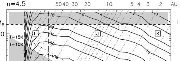
Figure 6: Same as Figure 5 but for $n=4.5$.

Dotted lines show the restriction imposed by the requirement that the gravitational binding energy of gas at the surface exceed the thermal energy for an estimated atmospheric temperature $T$ (Draine 1998):

$$M_{cl}>6\times 10^{-5}\left(\frac{T}{10{\rm K}}\right)~{}\left(\frac{R_{cl}}{{\rm AU}}\right)~{}M_{\odot}.$$ (29)

Two boundaries are shown, for atmospheric temperatures $T=10$ K and $T=15$ K. The shaded region below these curves is prohibited.

The thick solid lines are contours of constant event rate. The lensing rate is very high for all the cloud models appreciably to the right of the “rate $=0$” line.

Figures 7 and 8 show the results for the lensing rate for polytropes with $n=1.5$ and $n=4.5$ for a detection efficiency function approximately that of the MACHO experiment. All the notation is the same as in the case of $\phi_{\tau}=1$. The “rate $=0$” boundary has moved (relative to Figures 5 and 6) because we now require a threshold magnification $A_{t}=1.35$. Small glitches on the contours are artifacts of the numerical procedure. We consider here the events with all timescales filtered through the detection efficiency function discussed in Appendix B.

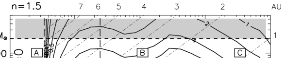
Figure 7: Contour plot of the event rate of gaseous lensing for various parameters of the lensing clouds, for the MACHO detection efficiency function. Polytrope $n=1.5$ is assumed and threshold magnification $A_{t}=1.35$. All the symbols and lines are the same as in Figure 5. Note the substantial decrease of the event rate due MACHO’s reduced sensitivity to short timescale events.

The rate which would be seen by the MACHO experiment is significantly smaller than the rate for $A_{t}=1.1$ and $\phi_{\tau}=1$, sometimes by two orders of magnitude. This is primarily a consequence of the reduced sensitivity to short timescale events of the MACHO detection efficiency function. Nevertheless the predicted rate is still quite high and in the next subsection we compare the predicted rate to that actually observed.

4.4 Comparison with the MACHO results

How shall we compare the results of the MACHO experiment with our simulated plot of what it would see if the dark matter is composed of molecular clouds? First of all, we need to estimate what fraction of the events actually observed by MACHO could be attributed to gaseous lensing. This can be done by noticing that the typical timescale of gaseous lensing events is very small, while the shortest timescale event reported by MACHO has $\hat{t}=34$ days. For the types of timescale distribution seen in Figures 3 and 4 it is extremely unlikely that there are more than $1$ or $2$ gaseous lensing events among those observed by MACHO, since otherwise a large number of short timescale events (with durations less than $10$ days) would be seen, in conflict with the distribution of timescales observed by the MACHO and EROS (Alcock et al. 2000; Lasserre et al. 2000) collaborations. It would also be completely inconsistent with the EROS and MACHO combined limits on the rate of very short timescale events, from $15$ minutes to several days, for which they claim that the analysis of two years of data on $8.6$ million stars found no short-duration “spike” events (Alcock et al. 1998), implying an upper limit $\dot{N}\leq 10^{-7}$ events yr^-1.

The MACHO collaboration observed $11.9$ million stars in the LMC for $5.7$ years. This means that the rate which could possibly be due to gaseous lensing events can be at most $(0.01-0.03)\times 10^{-6}~{}{\rm events}~{}{\rm yr}^{-1}$. It is clear from our simulated observations of gaseous lensing on Figures 7 and 8 that if $f_{cl}\geq 0.1$ the contour describing such a rate will lie very close to the line $S_{max}=S_{det}$, where the event rate drops to $0$. Any cloud model with $S_{max}<S_{det}$ will of course be undetectable and thus be allowed. Models with $S_{max}>1.1S_{det}$ are prohibited, because otherwise MACHO would have seen an enormous number of gaseous lensing events.

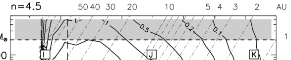
Figure 8: Same as Figure 7 but for $n=4.5$. Notice another allowed region at small cloud radii, bounded by contour corresponding to the event rate $3\times 10^{-8}~{}{\rm events}~{}{\rm yr}^{-1}$ and line $M=10^{-1.7}~{}M_{\odot}$.

These considerations and the restrictions described in §4.3 are combined together to produce an exclusion plot (Figure 9). One can see that an allowed region exists where clouds basically cannot be seen by the MACHO experiment and are not prohibited by the maximum mass and “thermal evaporation” constraints. For larger $n$ (softer equation of state) the allowed region shrinks. It is likely that for $n\to 5$ this region disappears completely, though we did not run our calculations for $n$ larger than $4.5$.

Also in the case $n=4.5$ another allowed region appears for small cloud radii (see Figure 8). It is bounded by the level contour corresponding to the rate $3\times 10^{-8}~{}{\rm events}~{}{\rm yr}^{-1}$ and goes into the region of the small cloud radii (see Figure 9 b).

The allowed regions can be further narrowed by noting that clouds are highly unlikely to have high central temperatures. Detailed studies of their thermal structure are not available, but it seems reasonable to exclude models of clouds with central temperatures $>(50-100)$ K. For $n=1.5$ this places another limit within the allowed region (see Figure 9a). In the case $n=4.5$ the allowed region for small radii virtually disappears because of this restriction (see Figure 9b).

In the absence of realistic models for the thermal structure of these clouds, we can only use $n=1.5$ polytropes as the most conservative model from the standpoint of gaseous lensing. For this case, we see that the allowed region is quite substantial, and contains the model with $M_{cl}=10^{-3}M_{\odot}$ and $R_{cl}=10$ AU which was favored by Draine (1998).

It is also possible to expand the allowed region by assuming that the clouds contribute only a small part $f_{cl}\ll 1$ of the dark matter (see §4.1), but to get any significant effect we need to suppose that this fraction is $<10^{-2}$ which would rule out these clouds as a main constituent of the dark matter, and eliminate them as the explanation for the extreme scattering events.

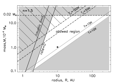
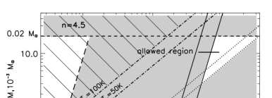
Figure 9: Exclusion plot for cloud radius $R_{cl}$ and mass $M_{cl}$, showing region of allowed parameters (unshaded) and prohibited (shaded regions) for clouds with polytropic index a) $n=1.5$ and b) $n=4.5$. Dotted lines represent limitation set by requirement that the atmosphere be gravitationally bound. Dashed line shows mass restriction by Wardle & Walker (1999). Region above the dash-dotted lines contains models with central temperature larger than $50$ K and $100$ K, respectively, which might exclude them (line shading). Note that another allowed region appears for small cloud radii in the $n=4.5$ case, bounded by dashed line roughly corresponding to the event rate $3\times 10^{-8}~{}{\rm events}~{}{\rm yr}^{-1}$ and line $M=10^{-1.7}~{}M_{\odot}$. As discussed in the text, the $n=1.5$ polytropic model is the most conservative assumption in the absence of detailed thermal models for these clouds. Star on the $n=1.5$ plot shows the position of the cloud model with $R_{cl}=10$ AU and $M_{cl}=10^{-3}M_{\odot}$.

It is clear that our lensing restriction represented on Figure 9 is sensitive to the adopted density profile of an individual cloud, but it is relatively insensitive to changes in the spatial and velocity distributions of the dark matter, since changes in these parameters are unlikely to produce variations in the event rate of $\geq 2$ orders of magnitude, which would be needed to move the restriction given by the observed lensing rate significantly away from the line “rate $=0$”.

5 Discussion

Wardle & Walker (1999) suggested that heating caused by cosmic rays in the cold molecular clouds can be balanced if particles of solid H₂ can form. They argue that these particles cool the cloud by thermal continuum radiation if the cloud mass lies in the range $10^{-7.5}-10^{-1.7}M_{\odot}$. Our calculations show that the lensing event rate would grow to extremely high values for masses below $10^{-4}M_{\odot}$ (see Figures 7 and 8 ).

Kalberla, Shchekinov, & Dettmar (1999) proposed that the $\gamma$-ray background emission from the Galactic halo seen in EGRET ($E>100$ MeV photons) data can be produced by interaction of high-energy cosmic rays with small dense clouds. They modeled this effect with different types of spatial distribution of dark matter in the form of these clouds and found that their best fit to the EGRET data for uniform density clouds occurred for $M_{cl}/R_{cl}^{2}\approx 10^{-3}~{}M_{\odot}/(6~{}AU)^{2}$. Their conclusions about the cloud parameters are model dependent, but the quoted values fall within the allowed range on Figure 9 for $n=1.5$.

Though it is impossible to observe the gravitational microlensing by the molecular clouds in our Galaxy it becomes possible if one observes them in other galaxies. A search for such lenses in the Virgo cluster is now underway (Tadros, Warren, & Hewett 2000) and preliminary results indicate that galaxy halos are unlikely to primarily consist of object with masses smaller than $10^{-5}~{}M_{\odot}$. We confirm this restriction but also place more rigorous constraints on the cloud properties since we can reject many models with higher cloud masses.

Another possible approach would be to look for periods of demagnification in the light curves of lensing events. For instance, the OGLE-II survey (Udalski et al. 1997) has collected a large sample of light curves for stars in the Galactic bulge, including $\sim 300$ lensing events (Woźniak 2000). Of these, two or three appear to show demagnification preceding or following the central peak in brightness, although the statistical significance of the demagnification has not yet been established (Woźniak, private communication). Demagnification cannot be produced by gravitational lensing by one or more point masses, but would be a characteristic signature of gaseous lensing.

6 Summary

In this paper we have considered in detail the lensing of stars in the LMC by small self-gravitating molecular clouds which have been proposed as a candidate for the dark matter in the Galaxy. Lensing would occur because of the refraction of optical light in the clouds, with resulting magnification of the source. We have developed a semianalytical formalism for calculation of the lensing rate including the spatial distribution of the dark matter, finite velocity dispersions of the lensing clouds and the source stars in LMC, and proper motion of the observer and LMC itself.

Our calculations were carried out for a single mass and size cloud population. One can easily extend the analysis to a distribution of cloud masses and sizes by simply convolving event rates obtained for a uniform cloud population with the appropriate distributions.

Lensing events might be detectable by searches for gravitational microlensing. This has allowed us to obtain constraints on the cloud properties by comparing our calculations with observational results obtained by the MACHO collaboration.

We found that almost the only possibility for the dark matter to be in the form of such molecular clouds is for the clouds to be sufficiently weak lenses so that their lensing effects are below the detection threshold of the MACHO experiment, since otherwise a very large gaseous lensing event rate would have been detected. This still leaves an allowed region in parameter space where these clouds could exist and not contradict the limitations posed by lensing experiments and simple physical considerations.

Though we have performed event rate calculations for only one halo model [given by equation (26)], we expect our results to be relatively insensitive to the particular form of the spatial distribution of these clouds, or the assumed shape of the velocity distribution of the clouds and the stars in the LMC.

Future microlensing experiments with a lower detection threshold magnification $A_{t}$ could either detect these clouds or strengthen the constraints on their properties.

7 Acknowledgements

We thank B.Paczyński and P.Woźniak for very helpful discussions, and R.H.Lupton for availability of the SM plotting package. This research has been supported in part by NSF grants AST-9619429 and AST-9988126.

Appendix A Derivation of equations (19) - (23)

For the purposes of the lensing rate calculations the velocities of the lens, observer, and source along the line of sight are not important, because only transverse motions are significant. It means that we can immediately perform integrations in equation (16) over $v_{Sz}$ and $v_{Lz}$.

Taking into account (15) we can perform integration over $\varphi$ in (16) and define the result as a function $\kappa({\bf v}_{\perp})$:

$$\kappa({\bf v}_{\perp})\equiv\frac{1}{\delta(x,A_{t})}\int\limits^{\delta(x,A_{t})}_{0}\phi_{\tau}(\tau(\varphi))d\varphi=\int\limits^{1}_{0}\phi_{\tau}\left(\frac{2\delta(x,A_{t})D_{OL}}{|{\bf v}_{\perp}|}\sqrt{1-s^{2}}\right)ds,$$ (A1)

so that now

$$d\dot{N}=2\delta\frac{\Sigma_{S}}{D_{OL}}\int\limits^{\infty}_{-\infty}dv_{Lx}\int\limits^{\infty}_{-\infty}dv_{Ly}\int\limits^{\infty}_{-\infty}dv_{Sx}\int\limits^{\infty}_{-\infty}dv_{Sy}|{\bf v}_{\perp}|f_{L}(v_{Lx},v_{Ly})f_{S}(v_{Sx},v_{Sy})\kappa(|{\bf v}_{\perp}|).$$ (A2)

We now change variables from $v_{Lx}$ and $v_{Ly}$ to $v_{x}$ and $v_{y}$ via equation (14):

$$d\dot{N}=2\delta\frac{d\Sigma_{L}}{\pi^{2}\sigma_{L}^{2}\sigma_{S}^{2}D_{OL}}\int\limits^{\infty}_{-\infty}dv_{x}\int\limits^{\infty}_{-\infty}dv_{y}\int\limits^{\infty}_{-\infty}dv_{Sx}\int\limits^{\infty}_{-\infty}dv_{Sy}\sqrt{v_{x}^{2}+v_{y}^{2}}\kappa(\sqrt{v_{x}^{2}+v_{y}^{2}})$$

$$\times\exp\left\{-\frac{(v_{x}-(1-x)v_{Ox}-xv_{Sx})^{2}+(v_{y}-xv_{Sy})^{2}}{\sigma_{L}^{2}}-\frac{(v_{Sx}-v_{cx})^{2}+(v_{Sy}-v_{cy})^{2}}{\sigma_{S}^{2}}\right\}.$$ (A3)

We integrate over $v_{Sx}$ and $v_{Sy}$ to obtain after lengthy but straightforward calculations

$$d\dot{N}=2\delta\frac{\Sigma_{S}}{\pi(\sigma_{L}^{2}+x^{2}\sigma_{S}^{2})D_{OL}}\int\limits^{\infty}_{-\infty}dv_{x}\int\limits^{\infty}_{-\infty}dv_{y}\sqrt{v_{x}^{2}+v_{y}^{2}}\kappa(\sqrt{v_{x}^{2}+v_{y}^{2}})$$

$$\times\exp\left\{-\frac{v_{x}^{2}+v_{y}^{2}}{\sigma_{L}^{2}+x^{2}\sigma_{S}^{2}}+\zeta_{1}v_{x}+\zeta_{2}v_{y}-C\right\},$$ (A4)

where

$$C=\frac{x^{2}v_{cy}^{2}+(xv_{cx}+(1-x)v_{Ox})^{2}}{\sigma_{L}^{2}+x^{2}\sigma_{S}^{2}},$$ (A5)

$$\zeta_{1}=2\frac{xv_{cx}+(1-x)v_{Ox}}{\sigma_{L}^{2}+x^{2}\sigma_{S}^{2}},~{}~{}~{}~{}~{}~{}~{}~{}~{}~{}\zeta_{2}=2\frac{xv_{cy}}{\sigma_{L}^{2}+x^{2}\sigma_{S}^{2}}.$$ (A6)

Introducing polar coordinates in velocity space $v_{x}=v\cos\beta$, $v_{y}=v\sin\beta$ and normalizing $v$ to some characteristic velocity $v_{ch}$ we get

$$d\dot{N}=2\delta\frac{\Sigma_{S}v_{ch}^{3}}{\pi(\sigma_{L}^{2}+x^{2}\sigma_{S}^{2})D_{OL}}e^{-C}\int\limits^{\infty}_{0}du~{}u^{2}\kappa(uv_{ch})e^{-Au^{2}}\int\limits^{2\pi}_{0}e^{uv_{ch}(\zeta_{1}\cos\beta+\zeta_{2}\sin\beta)}d\beta,$$ (A7)

where

$$A=\frac{v_{ch}^{2}}{\sigma_{L}^{2}+x^{2}\sigma_{S}^{2}}.$$ (A8)

The last integral in equation (A7) can be reduced to

$$\int\limits^{2\pi}_{0}e^{uv_{ch}\sqrt{\zeta_{1}^{2}+\zeta_{2}^{2}}cos(\beta+\beta_{0})}d\beta=\int\limits^{2\pi}_{0}e^{uv_{ch}\sqrt{\zeta_{1}^{2}+\zeta_{2}^{2}}cos\beta}d\beta=2\pi I_{0}\left(Bu\right),$$ (A9)

where $I_{0}$ is the modified Bessel function of order zero, and

$$B=v_{ch}\sqrt{\zeta_{1}^{2}+\zeta_{2}^{2}}=\frac{2v_{ch}}{\sigma_{L}^{2}+x^{2}\sigma_{S}^{2}}\sqrt{x^{2}v_{cy}^{2}+(xv_{cx}+(1-x)v_{Ox})^{2}}=2\sqrt{AC}.$$ (A10)

So, finally we get for the event rate produced by one lens

$$d\dot{N}(x)=4\delta\frac{\Sigma_{S}v_{ch}^{3}}{(\sigma_{L}^{2}+x^{2}\sigma_{S}^{2})D_{OL}}e^{-C}\int\limits^{\infty}_{0}u^{2}\kappa(uv_{ch})e^{-Au^{2}}I_{0}\left(Bu\right)du.$$ (A11)

Thus, the total event rate per source, produced by all lenses between us and LMC, is given by formula (19).

Now, we obtain the formula for the timescale distribution (22). Note that $\tau$ and $\varphi$ – the angular distance from the lens’s trajectory to the source star in the perpendicular direction – are directly related by equation (15):

$$d\varphi=-\delta(x,A_{t})\frac{d\tau}{\tau}\frac{u^{2}}{\sqrt{1-u^{2}}},$$ (A12)

with $u=v_{\perp}/v_{ch}$, $v_{ch}=2b_{0t}(x,A_{t})/\tau$. To obtain $d\dot{N}_{tot}/d\tau$ we simply omit the integration over $\varphi$ in (16). Also, the velocity $v_{\perp}$ is limited by $2b_{0t}(x,A_{t})/\tau$. All the other steps are analogous to those which we have done in derivation of (19) and we obtain equation (22).

If we are interested only in events whose durations are larger than some chosen value $\tau_{min}$, then to get the total rate we should integrate in (16) over $\varphi$ not up to $\delta(x,A_{t})$, but up to

$$\varphi_{max}=\sqrt{\delta^{2}-\frac{v_{\perp}^{2}\tau_{min}^{2}}{4D_{OL}}}=\delta\sqrt{1-u^{2}},$$ (A13)

with $u=v_{\perp}\tau/2\delta xD$. One can easily see that we will get in this case for $\dot{N}_{tot}(\tau>\tau_{min})$ the formula (23).

Appendix B Detection efficiency function

The detection efficiency function $\phi$ characterizes the sensitivity of the experiment to events with different durations. We will use the detection efficiency $\phi_{\hat{t}}(A,\hat{t})$ assumed by MACHO experiment to estimate how it would affect gaseous lensing (see Figure 8 in Alcock et al. (1997)).

We first recall some simple facts about gravitational microlensing. The amplification $M$ in the case of gravitational microlensing is determined by the formula

$$M(u)=\frac{u^{2}+2}{u(u^{2}+4)^{1/2}},~{}~{}~{}~{}u=(u_{min}^{2}+4t^{2}/\hat{t}^{2})^{1/2}$$

$$u_{min}=\frac{b_{min}}{r_{E}},~{}~{}~{}~{}\hat{t}=2\frac{r_{E}}{v_{\perp}},~{}~{}~{}~{}r_{E}=\left[\frac{4GmDx(1-x)}{c^{2}}\right]^{1/2},$$ (B1)

where $b_{min}$ is the impact parameter, $m$ is the mass of the lensing object, $t$ is the time of observation, and $v_{\perp}$ is, again, the relative velocity of the lens and the source star.

Recall that we defined the timescale $\tau$ to be the time spent with magnification $M>A_{t}$. From equation (B1) we find that, for gravitational microlensing,

$$\tau_{gm}=\sqrt{2}\hat{t}\left[\frac{A_{t}}{\sqrt{A_{t}^{2}-1}}-\frac{A_{max}}{\sqrt{A_{max}^{2}-1}}\right]^{1/2}$$

$$=\hat{t}\left[u_{t}^{2}-u_{min}^{2}\right]^{1/2},$$ (B2)

where $u_{t}$ is the value of $u$ at which the magnification is equal to $A_{t}$ and $A_{max}$ is the maximum magnification for a given $u_{min}$.

We use a very simple algorithm for converting detection efficiency function from $\hat{t}$ to $\tau$: since $\tau\propto\hat{t}$, their ratio $\tau/\hat{t}$ is a function of $A_{max}$ (or $u_{min}$) for a given $A_{t}$. Thus we can average this ratio over the distribution of the maximum magnifications $A_{max}$ and assume that the value of known $\phi_{\hat{t}}(\hat{t})$ is equal to the $\phi_{\tau}(<\tau>)$, that is

$$\phi_{\tau}(\tau)=\phi_{\hat{t}}\left(\tau\left(<\tau/\hat{t}>\right)^{-1}\right).$$ (B3)

The calculation of $<\tau/\hat{t}>$ is quite straightforward and can be most easily done in terms of $u_{min}$ (see the last equality in equation (B2)). Since the distribution of lensing events over $u_{min}$ is just constant

$$<\tau/\hat{t}>=\frac{\int\limits^{u_{t}}_{0}\left[u_{t}^{2}-u_{min}^{2}\right]^{1/2}du_{min}}{\int\limits^{u_{t}}_{0}du_{min}}=\frac{\pi}{4}u_{t}=\frac{\pi}{2\sqrt{2}}\left(\frac{A_{t}}{\sqrt{A_{t}^{2}-1}}-1\right)^{1/2}.$$ (B4)

For $A_{t}=1.35$, accepted by MACHO experiment, $<\tau/\hat{t}>=0.776$, which means that $\phi_{\tau}(\tau)=\phi_{\hat{t}}(1.288\tau)$.

References

- (1)
- (2) Alcock, C., et al. 1997, ApJ, 486, 697
- (3)
- (4) Alcock, C., et al. 1998, ApJL, 499, L9
- (5)
- (6) Alcock, C., et al. 2000, ApJ, 542, 281
- (7)
- (8) American Institute of Physics Handbook. 1972, ed. D.E.Gray (New York: McGraw-Hill)
- (9)
- (10) De Paolis, F., Ingrosso, G., Jetzer, Ph., & Roncadelli, M. 1995a, PhRvL, 74, 14
- (11)
- (12) De Paolis, F., Ingrosso, G., Jetzer, P., & Roncadelli, M. 1995b, A&A, 295, 567
- (13)
- (14) De Paolis, F., Ingrosso, G., Jetzer, P., & Roncadelli, M. 1996, Ap&SS, 235, 329
- (15)
- (16) Draine, B.T. 1998, ApJ, 509, L41
- (17)
- (18) Fiedler, R., Dennison, B., Johnston, K.J., Waltman, E.B., & Simon, R.S. 1994, ApJ, 430, 581
- (19)
- (20) Freese, K., Fields, B., & Graff, D. 2000, astro-ph/0002058
- (21)
- (22) Gerhard, O., & Silk, J. 1996, ApJ, 472, 34
- (23)
- (24) Gould, A. & Andronov, N. 1999, ApJ, 516, 236
- (25)
- (26) Griest, K. 1991, ApJ, 366, 412
- (27)
- (28) Han, C. & Gould, A. 1996, ApJ, 467, 540
- (29)
- (30) Henriksen, R.N., & Widrow, L.M. 1995, ApJ, 441, 70
- (31)
- (32) Jones, B.F., Klemola, A.R., & Lin, D.N.C. 1994, AJ, 107, 1333
- (33)
- (34) Kalberla, P.M.W., Shchekinov, Yu.A., Dettmar, R.-J. 1999, A&A, 350, L9
- (35)
- (36) Lasserre, T. et al. 2000, A&A, 355, L39
- (37)
- (38) Navarro, J.F., Frenk, C.S., & White, S.D.M. 1996, ApJ, 462, 563
- (39)
- (40) Paczyński, B. 1996, ARA&Ap, 34, 419
- (41)
- (42) Pfenniger, D. Combes, F., & Martinet, L. 1994, A&A, 285, 79
- (43) Sciama, D.W. 2000, MNRAS, 312, 33
- (44)
- (45) Tadros, H., Warren, S.J., & Hewett, P.C. 2000, astro-ph/0003422
- (46)
- (47) Udalski, A., Kubiak, M., & Szymanski, M. 1997, Acta Astronomica, 47, 319
- (48)
- (49) Walker, M., & Wardle, M. 1998, ApJL, 498, L125
- (50)
- (51) Walker, M. 1999, MNRAS, 308, 551
- (52)
- (53) Wardle, M. & Walker, M. 1999, ApJL, 527, L109
- (54)
- (55) Widrow, L.M. & Dubinski, J. 1998, ApJ, 504, 12
- (56)
- (57) Woźniak, P. 2000, in preparation
- (58)