ABSTRACT

The observables $T/S$ and $n-1$ are key to testing and understanding inflation. ($T$, $S$, and $n-1$ respectively quantify the gravity-wave and density-perturbation contributions to CMB anisotropy and the deviation of the density perturbations from the scale-invariant form.) Absent a standard model, there is no definite prediction for, or relation between, $T/S$ and $n-1$. By reformulating the equations governing inflation we show that models generally predict $T/S\approx-5(n-1)$ or $0$, and in particular, if $n>0.85$, $T/S$ is expected to be $>10^{-3}$.

Introduction. Cosmic microwave background (CMB) anisotropy measurements have begun to test inflation, the leading paradigm to extend the standard big-bang cosmology. Within a decade they should test inflation decisively and even probe the underlying physics [1, 2, 3]. Recent results from the BOOMERanG and MAXIMA CMB experiments [4, 5] (as well as results from earlier experiments [6]) confirm the flat Universe predicted by inflation and are beginning to address its second basic prediction: almost scale-invariant adiabatic, Gaussian density perturbations produced by quantum fluctuations during inflation [7]. The third prediction, a nearly scale-invariant spectrum of gravity waves, will be more difficult to confirm, but is a critical probe of inflation [8].

The key inflationary observables are: the level of anisotropy arising from density (scalar) perturbations (quantified by the contribution to the CMB quadrupole anisotropy, $S$), the level of anisotropy arising from gravity-wave (tensor) perturbations ($T$), and the power-law index $n$ that characterizes the density perturbations (scale invariance refers to equal amplitude fluctuations in the gravitational potential on all length scales and corresponds to $n=1$). If $T$, $S$ and $n-1$ can be measured, then the scalar-field potential that drove inflation can be reconstructed [10]. The most promising means of measuring $T$ is its unique signature in the polarization of CMB anisotropy [9] (however, direct detection by a future space-based experiment should not be dismissed).

While there is no standard model of inflation, all known models can be cast in terms of the classical evolution of a new scalar field $\phi$ (dubbed the inflaton) [13]. Predictions for $S$, $T$ and $n-1$ can be expressed in terms of the scalar-field potential $V(\phi$) and its first two derivatives. While there is a model-independent relation between $T/S$ and the power-law index $n_{T}$ that characterizes the gravity-wave spectrum, $T/S=-5n_{T}$ [11, 12], no such relation for $n$ and $T/S$ exists [14].

This is unfortunate because $n_{T}$ is very difficult to measure, and $n$ will be measured to a precision of better than 1% by the MAP and PLANCK experiments (BOOMERanG and MAXIMA have already determined that $n=1\pm 0.06$). Even an approximate or generic relation between $(n-1)$ and $T/S$ would be valuable, both as a test of inflation and as a guide for the expected level of gravity waves when $n$ is measured.

The formation of large-scale structure and CMB measurements already indicate that a significant part of CMB anisotropy arises from scalar perturbations ($T/S$ cannot be $\gg 1$). On the other hand, nothing precludes $T/S\ll 1$, and if $T/S$ is much less than $10^{-3}$, the prospects for measuring $T$ are poor [9] (one inflation theorist has opined that $T/S\ll 1$ for all reasonable models [15]).

The goal of this work is to provide objective theoretical guidance. By casting the equations governing inflation in a form that is essentially independent of the inflaton potential (“flow equations” for $T/S$ and $n-1$), we show that the $T/S$ – $(n-1)$ plane is not uniformly populated by models of inflation: The lines $T/S\approx 0$ and $T/S\approx-5(n-1)$ act as attractors for models that are consistent with the equations governing inflation. For $n<1$, there is an excluded region between these two attractors; for $n>1$, other values for $T/S$ and $n-1$ are possible, but at the expense of a spectrum of density perturbations that is poorly represented by a power law. (the CMB will be able to test how well a power law describes the density perturbations.)

Flow equations. The kinematic equations that govern inflation are well known [16]

$$\ddot{\phi}+3H\dot{\phi}+V^{\prime}(\phi) = 0$$ (1)

$$H^{2}\equiv\left(\frac{\dot{a}}{a}\right)^{2} = \frac{8\pi}{3{m_{\rm Pl}}^{2}}\left[V(\phi)+\frac{1}{2}\dot{\phi}^{2}\right]$$ (2)

where $a(t)$ is the cosmic scale factor, prime denotes $d/d\phi$, and overdot denotes $d/dt$. During inflation $\phi$ rolls slowly and the $\ddot{\phi}$ term in its equation of motion and its kinetic term in the Friedmann equation can be neglected [16, 17], so that

$$\dot{\phi} \simeq \frac{-V^{\prime}}{3H}$$ (3)

$$N(\phi)\equiv\int^{\phi_{\rm end}}_{\phi}Hdt \simeq -\frac{8\pi}{{m_{\rm Pl}}^{2}}\int_{\phi}^{\phi_{\rm end}}\frac{d\phi}{x(\phi)}$$ (4)

where $x(\phi)\equiv V^{\prime}(\phi)/V(\phi)$ measures the steepness of the potential and $N(\phi)$, the number of e-folds before the end of inflation, is the natural time variable. Inflation ends when the slow-roll conditions,

$${m_{\rm Pl}}V^{\prime}/V={m_{\rm Pl}}x < \sqrt{48\pi}$$ (5)

$${m_{\rm Pl}}^{2}V^{\prime\prime}/V={m_{\rm Pl}}^{2}(x^{\prime}+x^{2}) < 24\pi\,,$$ (6)

are violated (at $\phi=\phi_{\rm end}$) [16, 17].

The inflationary observables are related to the same quantities that govern the kinematics of inflation [12]

$$(n-1) = \frac{{m_{\rm Pl}}^{2}}{8\pi}\left[2x^{\prime}-x^{2}\right]$$ (7)

$$T/S = \frac{5{m_{\rm Pl}}^{2}}{8\pi}x^{2}$$ (8)

$$T = 0.6V/{m_{\rm Pl}}^{4}$$ (9)

These expressions are given to lowest order in $x^{2}$ and $x^{\prime}$ (see Ref. [18] for higher-order corrections). Note, $n-1$ is only equal to $n_{T}=-5(T/S)$ if $x^{\prime}=0$.

By combining the slow-roll equations with those governing $(n-1)$ and $T/S$, we can write equations that govern the inflationary observables (almost) without reference to a model,

$$\frac{d(T/S)}{dN} = (n-1)\frac{T}{S}+\frac{1}{5}\left(\frac{T}{S}\right)^{2}$$ (10)

$$\frac{d(n-1)}{dN} = -\frac{1}{5}(n-1)\frac{T}{S}-\frac{1}{25}\left(\frac{T}{S}\right)^{2}\pm\frac{{m_{\rm Pl}}^{3}}{16\pi^{2}}\sqrt{\frac{2\pi}{5}\frac{T}{S}}\,x^{\prime\prime}$$ (11)

where the sign of the last term matches that of $V^{\prime}$.

We call these “flow equations” as they describe the trajectory in the $T/S$ – $(n-1)$ plane during inflation. Because of the $x^{\prime\prime}$ term they are not completely independent of the potential. To “close” the flow equations we will assume that the potential is smooth enough so that we can treat $x^{\prime\prime}$ as being approximately constant. For sufficiently smooth and featureless potentials $x^{\prime\prime}$ will also be small.

Finally, one might wonder what happened to the most stringent constraint on inflation: achieving density perturbations of amplitude $10^{-5}$ or so ($S\sim 10^{-10}$). The flow equations involve the quantities $T/S$, $(n-1)$ and $dN/d\phi$ which are unaffected by a rescaling of the potential, $V\rightarrow aV$. This rescaling changes $S$: $S\rightarrow aS$. Thus, any potential can be rescaled to give proper size density perturbations without affecting the flow equations.

Trajectories and attractors. The scales relevant for structure formation ($1\,{\rm Mpc}$ to $10^{4}\,{\rm Mpc}$) crossed outside the horizon roughly 50 $e$-folds before the end of inflation (i.e., when $N=50$) [16], and so it is $T/S$ and $(n-1)$ at this time that can be measured by CMB experiments. We find them by evolving $T/S$ and $(n-1)$ until inflation ends and counting back 50 e-folds. To determine when inflation ends, we recast the slow-roll conditions (5,6):

$$T/S < 30$$ (12)

$$\left|(n-1)+\frac{3}{5}\frac{T}{S}\right| < 6$$ (13)

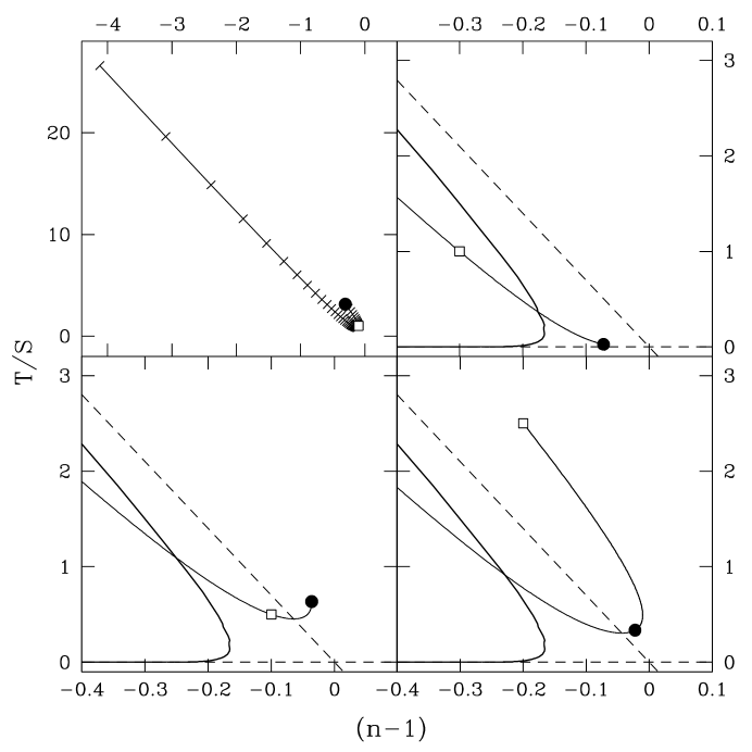
Figure 1: Trajectories in the $T/S$ – $(n-1)$ plane. Squares indicate the initial choices for $T/S$ and $(n-1)$; circles indicate the values 50 e-folds before the end of inflation. A trajectory ends when $T/S$ and/or $|n-1|$ become large; most of inflation occurs when $T/S$ and $|n-1|$ are small. The upper left panel shows a complete trajectory, with ticks indicating e-folds before the end of inflation (from the circle, $50,49,\cdots,1$). The other three panels show trajectories in more detail. Note how $T/S$ and $(n-1)$ outside the attractor region are “pulled in” (the attractors are shown as broken lines and the boundary of the excluded region is a solid curve).

To be specific, we pick “initial” values in the range, $0<T/S<10$ and $-0.5<(n-1)<0.5$, and then integrate with fixed $x^{\prime\prime}$ until one of the slow-roll conditions is violated, signaling the end of inflation. We then count back 50 $e$-folds to find $(T/S)_{50}$ and $(n-1)_{50}$. Some trajectories are shown in Fig. 1.

Figs. 2 and 3 summarize the $(T/S)_{50}$ – $(n-1)_{50}$ phase space generated from the range of initial conditions considered. The $(T/S)_{50}$ – $(n-1)_{50}$ plane is not uniformly populated. For $x^{\prime\prime}<{\cal O}(1)$, solutions cluster around two attractors, $(T/S)_{50}\approx 0$ and $(T/S)_{50}\approx-5(n-1)_{50}$, and for $(n-1)_{50}<0$, there is an excluded region between the two attractor lines, which cannot be reached for any value of $x^{\prime\prime}$. We call the region between the excluded area and $x^{\prime\prime}=3$ as the favored region for the inflationary observables $n-1$ and $T/S$.

Taking $x^{\prime\prime}=0$ it is simple to show how the attractors arise. In this limit, the flow equations are: $s\equiv(n-1)-{1\over 5}{T\over S}=\,$const and $r\propto\exp(sN)$, where $r=T/S$. Unless $r$ and /or $s$ are small, corresponding to the attractor solutions, $r$ grows very rapidly and inflation does not last 50 e-folds.

For $n>1$, values of $(T/S)$ and $(n-1)$ outside the favored region are possible at the expense of large $x^{\prime\prime}$. Models with a large $x^{\prime\prime}$ have density-perturbation spectra which are not well represented by a power law: the running of the spectral index [20], $dn/d\ln k=-dn/dN$ includes the term

$${dn\over d\ln k}=\cdots\pm{{m_{\rm Pl}}^{3}\over 16\pi^{2}}\sqrt{{2\pi\over 5}{T\over S}}\,x^{\prime\prime}$$ (14)

which becomes large for large $x^{\prime\prime}$. This explains the results of a recent paper [21] in which models with $n$ as large as 2 were constructed. In particular, for the model with $n=2$, $x^{\prime\prime}\simeq 2000$, $T/S\simeq 3\times 10^{-3}$ and $dn/d\ln k\simeq 0.3$.

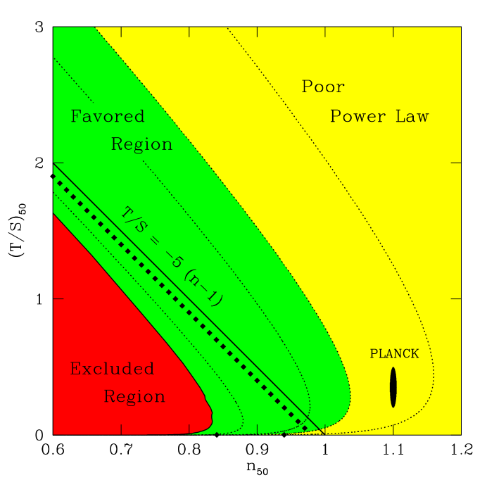
Figure 2: Summary of our model search using the flow equations. The lines $T/S=-5(n-1)$ and $T/S=0$ act as attractors; the dotted curves correspond to $x^{\prime\prime}=0,1,2,5$ (from left to right). We found no model in the excluded region, and we call the region between it and the curve $x^{\prime\prime}=3$ the favored region. Models outside the favored region (upper right part) have large $dn/d\ln k$ and density perturbations that are not well represented by a power law. Diamonds indicate various known inflationary models: chaotic, $V(\phi)=\lambda\phi^{n}$ for $n=2,3,\cdots$ (diamonds on the diagonal); new inflation ($n=0.94$) and natural inflation (with $n=0.84$). The ellipse is the $2\sigma$ error ellipse “forecasted” for the PLANCK satellite [19].

Fig. 3 shows the $T/S\approx 0$ attractor region in more detail. As $n$ increases toward unity, values of $T/S$ in the favored region grow, making the prospects for measuring $T$ better; in particular, for $n>0.85$, $T/S>10^{-3}$. This figure also confirms that almost, but not exactly, scale-invariant density perturbations are a generic prediction of inflation [7, 17]: the favored region just touches $n=1$ (for $x^{\prime\prime}\simeq 1.5$). Finally, in the disfavored region where $T/S\ll 1$, large $x^{\prime\prime}$ does not imply a poor power law because $dn/d\ln k$ is proportional to $T/S$. Indeed one of the models in this region is new inflation.

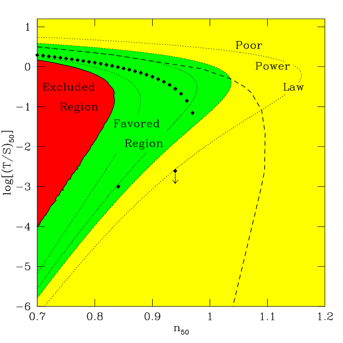
Figure 3: Same as Fig. 2, except with a logarithmic scale for $T/S$ to show more detail. As $n\rightarrow 1$, $T/S$ increases in the favored region. Below and to the left of the broken line ($dn/d\ln k=10^{-2}$), a poor power law does not occur for large $x^{\prime\prime}$ because $dn/d\ln k\propto\sqrt{T/S}\,x^{\prime\prime}$ and $T/S$ is small.

So far, we have only considered one-field inflation. There are potentials that are so flat and smooth that the slow-roll conditions never break down; the most well known of these is power-law inflation, $V(\phi)\propto\exp(-\beta\phi/{m_{\rm Pl}})$. In a “never ending” model, another field causes the slow-roll conditions to break down (e.g., by classical evolution in hybrid inflation or a phase transition in extended inflation). The flow equations can also be applied to such models.

In our framework two-field models are models that would inflate forever on their own. We find such models when the right hand sides of Eqs. (10,11) vanish prior to violating the slow-roll conditions. When this happens, we obtain fixed points in the $T/S$ – $(n-1)$ plane, which are the most likely values for $T/S$ and $(n-1)$ 50 $e$-folds prior to when the second field ends inflation. These points, shown in Fig. 4, populate the region $T/S\approx 0$ and for $n>1$ along with the attractor line, $T/S=-5(n-1)$.

It is also possible that a self-ending model has an auxiliary field that ends inflation “early”. We treat this possibility by populating the $(T/S)_{50}$ – $(n-1)_{50}$ plane with the values of $T/S$ and $(n-1)$ at $N>50$ for all one-field models. We find that the two-field models behave similarly to the one-field models. The only significant difference is that two-field models extend the $(T/S)_{50}=0$ attractor to $(n-1)_{50}>0$ (see Fig. 4).

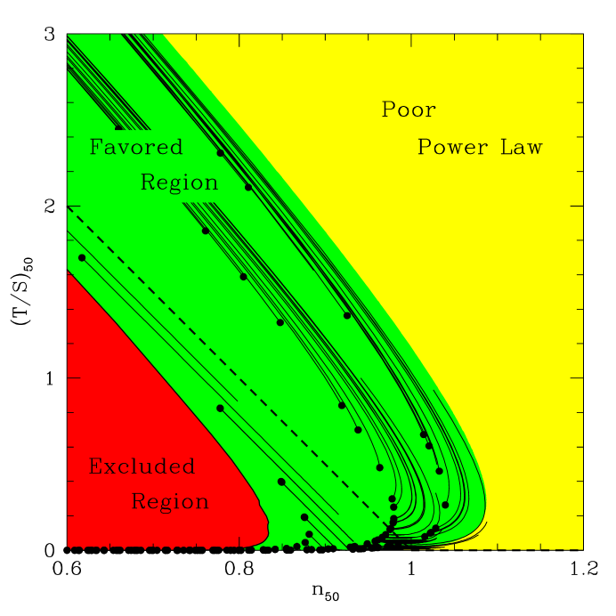
Figure 4: Summary of two-field models. The filled circles represent the values of $(T/S)_{50}$ and $n_{50}$ for the corresponding one-field models, and the attached curves are the values obtained for inflation ending early due to an auxiliary field. The dashed lines represent fixed points in the $(T/S)$ – $n$ plane that result from models that do not end without an auxiliary field. In general, two-field models populate the same region as one-field models and extend the $T/S\approx 0$ attractor to $n>1$.

Finally, what about our taking $x^{\prime\prime}\simeq\,$ constant? It can affect the relationship between the initial and final values of $n-1$ and $T/S$ if $x^{\prime\prime}$ is large, since $x^{\prime\prime}$ need not be constant (as is the case in some known models). Since we have covered a wide range of initial values we would expect that this fact would only slightly modify the $(n-1)_{50}$ – $(T/S)_{50}$ phase space; indeed, we have also formulated the flow equations assuming $V^{\prime\prime\prime}/V=\,$ constant and obtain similar results. Further, in the favored part of the $(n-1)_{50}$ – $(T/S)_{50}$ plane, $x^{\prime\prime}$ is small.

Discussion. Prior to this work there was one guiding relation for the inflationary observables: $T/S=-5n_{T}$. It has the virtue of exactitude and can test the consistency of the scalar-field inflationary framework, but it involves the power-law index of the gravity wave perturbations, the most difficult inflationary observable to measure. By reformulating the equations governing inflation, we have found generic relations between $T/S$ and $(n-1)$: Inflationary kinematics constrain models to cluster along the lines $T/S=-5(n-1)$ and $T/S=0$, with a forbidden region between these two lines for $n<1$. Large $n-1$ is possible, but at the expense of a poor power-law for the density perturbations (i.e., large $dn/d\ln k$), unless $T/S$ is very small. Further, our results support the view that inflation generically predicts almost, but not exactly scale-invariant density perturbations [17].

These results provide practical guidance to CMB experimenters and additional tests for inflation. For example, if $n$ is found to be significantly greater than 1, then a poor power-law is also expected unless $T/S\ll 1$. If $n$ is found to be $>0.85$, then $T/S>10^{-3}$ is likely, which would makes prospects for detecting the gravity-wave of inflation signature more favorable.

References

- [1] http://map.gsfc.nasa.gov/
- [2] http://astro.estec.esa.nl/SA-general/Projects/Planck/
- [3] http://www.sns.ias.edu/ whu
- [4] P. de Bernardis et. al., Nature 404, 955 (2000); A. Lange et al, astro-ph/0005004.
- [5] S. Hanany et al, astro-ph/0005123; A. Balbi et al, astro-ph/0005124.
- [6] See e.g., L. Knox and L. Page, astro-ph/0002162.
- [7] A.H. Guth and S.-Y. Pi, Phys. Rev. Lett. 49, 1110 (1982); S.W. Hawking, Phys. Lett. B 115, 295 (1982); A.A. Starobinskii, ibid 117, 175 (1982); J.M. Bardeen, P.J. Steinhardt, and M.S. Turner, Phys. Rev. D 28, 697 (1983).
- [8] V.A. Rubakov, M. Sazhin, and A. Veryaskin, Phys. Lett. B 115, 189 (1982); R. Fabbri and M. Pollock, ibid 125, 445 (1983); A.A. Starobinskii Sov. Astron. Lett. 9, 302 (1983); L. Abbott and M. Wise, Nucl. Phys. B 244, 541 (1984).
- [9] M.S. Turner, Phys. Rev. D 55, R435 (1996); M. Kamionkowski and A. Kosowsky, ibid 57, 685 (1998).
- [10] See e.g., J. Lidsey et al, Rev. Mod. Phys. 69, 373 (1997); M.S. Turner, Phys. Rev. D 48, 5539 (1993).
- [11] R. Davis, Phys. Rev. Lett. 69, 1856 (1992); D. Lyth and A. Liddle, Phys. Lett. B 291, 391 (1992).
- [12] The precise relationship between and and the inflaton potential depends upon the cosmological model; see M.S. Turner and M. White, Phys. Rev. D 53, 6822 (1996). The values used in this paper are for and . For , the relation is the more familiar .
- [13] See e.g., D. Lyth and A. Riotto, Phys. Rept. 314, 1 (1999).
- [14] It had been conjectured that for many models , though there are many exceptions to this; see R. Davis, Phys. Rev. Lett. 69, 1856 (1992) and V.F. Mukhanov, L. Wang and P.J. Steinhardt, Phys. Lett. B 414, 18 (1997).
- [15] D. Lyth, Phys. Rev. Lett. 78, 1861 (1997).
- [16] E.W. Kolb and M.S. Turner, The Early Universe (Addison-Wesley, Redwood City, CA 1990), Ch. 8.
- [17] P.J. Steinhardt and M.S. Turner, Phys. Rev. D 29, 2162 (1984).
- [18] A.R. Liddle and M.S. Turner, Phys. Rev. D 50, 758 (1994).
- [19] W.H. Kinney, Phys. Rev. D 58, 123506 (1998).
- [20] A. Kosowsky and M.S. Turner, Phys. Rev. D 52, R1739 (1995).
- [21] D. Huterer and M.S. Turner, Phys. Rev. D, in press (astro-ph/9908157).