How Many Galaxies Fit in a Halo?
Constraints on Galaxy Formation Efficiency from Spatial Clustering

Abstract

We study galaxy clustering in the framework of halo models, where gravitational clustering is described in terms of dark matter halos. At small scales, dark matter clustering statistics are dominated by halo density profiles, whereas at large scales, correlations are the result of combining non-linear perturbation theory with halo biasing. Galaxies are assumed to follow the dark matter profiles of the halo they inhabit, and galaxy formation efficiency is characterized by the number of galaxies that populate a halo of given mass. This approach leads to generic predictions: the galaxy power spectrum shows a power-law behavior even though the dark matter does not, and the galaxy higher-order correlations show smaller amplitudes at small scales than their dark matter counterparts. Both are in qualitatively agreement with measurements in galaxy catalogs. We find that requiring the model to fit both the second and third order moments of the APM galaxies provides a strong constraint on galaxy formation models. The data at large scales require that galaxy formation be relatively efficient at small masses, $m\approx 10^{10}M_{\sun}/h$, whereas data at smaller scales require that the number of galaxies in a halo scale approximately as the mass to the $0.8$th power in the high-mass limit. These constraints are independent of those derived from the luminosity function or Tully-Fisher relation. We also predict the power spectrum, bispectrum, and higher-order moments of the mass density field in this framework. Although halo models agree well with measurements of the mass power spectrum and the higher order $S_{p}$ parameters in N-body simulations, the model assumption that halos are spherical leads to disagreement in the configuration dependence of the bispectrum at small scales. We stress the importance of finite volume effects in higher-order statistics and show how they can be estimated in this approach.

1 Introduction

Understanding galaxy clustering is one of the main goals of cosmology. The wealth of information provided by galaxy surveys can only be used to extract useful cosmological information if we understand the relation between galaxy and dark matter clustering—biasing. On large enough scales, galaxy biasing can be described as a local process, and so galaxy clustering can be used as a direct probe of the primordial spectrum and Gaussianity of initial conditions (Fry & Gaztañaga 1993; Frieman & Gaztañaga 1994; Fry 1994; Fry & Scherrer 1994; Gaztañaga & Mähönen 1996; Matarrese, Verde & Heavens 1997; Gaztañaga & Fosalba 1998; Frieman & Gaztañaga 1999; Scoccimarro et al. 2000; Durrer et al. 2000). On smaller scales, however, non-negligible contributions from complex astrophysical processes relevant to galaxy formation may complicate the description of galaxy biasing.

Galaxy formation is not yet understood from first physical principles. However, following White & Rees (1978) and White & Frenk (1991), a number of prescriptions based on reasonable recipes for approximating the complicated physics have been proposed for incorporating galaxy formation into numerical simulations of dark matter gravitational clustering (see, e.g., Kauffmann et al. 1999, Somerville & Primack 1999 or Benson et al. 2000 for some of the most recent work). These “semianalytic galaxy formation” schemes can provide detailed predictions for galaxy properties in hierarchical structure formation models, which can then be compared with observations.

The basic assumption in the semianalytic approach is that galaxy biasing can be described as a two-step process. First, the formation and clustering of dark matter halos can be modeled by neglecting non-gravitational effects. This can be done reasonably accurately following the analytic results of Mo & White (1996), Mo, Jing & White (1997) and Sheth & Lemson (1999). Second, the distribution of galaxies within halos, which in principle depends on complicated physics, can be described by a number of simplifying assumptions regarding gas cooling and feedback effects from supernova. For the purposes of this paper, the main outcome of this second step is the number of galaxies that populate a halo of a given mass, $N_{\rm gal}(m)$.

In this paper we consider the problem of galaxy clustering from a complementary point of view to semianalytic models. We construct clustering statistics from properties of dark matter halos and the $N_{\rm gal}(m)$ relation, and show how these simple ingredients can be put together to make reasonably accurate analytic predictions about the galaxy power spectrum, bispectrum, and higher-order moments of the galaxy field. We also consider the inverse problem: we show how measurements of galaxy clustering can constrain the $N_{\rm gal}(m)$ relation. We show in particular that the variance and skewness of the galaxy distribution in the APM survey provide significant constraints on the $N_{\rm gal}(m)$ relation.

Our approach to gravitational clustering has a long history, dating back to Neyman, & Scott (1952), and then explored further by Peebles (1974), and McClelland & Silk (1977a,b;1978). These works considered perturbations described by halos of a given size and profile, but distributed at random. A complete treatment which includes the effects of halo-halo correlations was first given by Scherrer & Bertschinger (1991). Recent work has focused on applications of this formalism to the clustering of dark matter, e.g. the small-scale behavior of the two-point correlation function (Sheth & Jain 1997), the power spectrum (Seljak 2000; Peacock & Smith 2000; Ma & Fry 2000; Cooray & Hu 2000), and the bispectrum for equilateral configurations (Ma & Fry 2000; Cooray & Hu 2000). Interest in this approach has been undoubtedly sparked by recent results from numerical simulations on the properties of dark matter halos (Navarro, Frenk, & White 1996, 1997; Bullock et al. 1999; Moore et al. 1999).

This paper is organized as follows. In Section 2 we review the halo model formalism for the power spectrum, bispectrum and higher-order moments of the smoothed density field, and compare the predictions with numerical simulations in Section 3. We discuss in detail the role of finite volume effects which, if neglected, can lead to incorrect conclusions regarding higher-order statistics. In Section 4, we use the $N_{\rm gal}(m)$ relation to make predictions for galaxy, rather than dark matter, clustering statistics (also see Jing, Mo & Börner 1998; Seljak 2000; Peacock & Smith 2000). To illustrate our approach, we use the $N_{\rm gal}(m)$ relation obtained from the semianalytic models of Kauffmann et al. (1999). In Section 5 we discuss the constraints on $N_{\rm gal}(m)$ derived from analysis of counts-in-cells of the APM survey. Section 6 summarizes our conclusions.

2 Dark Matter Clustering

2.1 Formalism

In this section we follow the formalism developed by Scherrer & Bertschinger (1991). The dark matter density field is written as

$$\rho({\hbox{\BF x}})=\sum_{i}f({\hbox{\BF x}}-{\hbox{\BF x}}_{i},m_{i})\equiv\sum_{i}m_{i}\ u({\hbox{\BF x}}-{\hbox{\BF x}}_{i},m_{i})=\sum_{i}\int dmd^{3}x^{\prime}\delta(m-m_{i})\delta^{3}({\hbox{\BF x}}^{\prime}-{\hbox{\BF x}}_{i})mu({\hbox{\BF x}}-{\hbox{\BF x}}^{\prime},m),$$ (1)

where $f$ denotes the density profile of a halo of mass $m_{i}$ located at position ${\hbox{\BF x}}_{i}$. The mean density is

$$\bar{\rho}=\mathop{\langle}\rho({\hbox{\BF x}})\mathop{\rangle}=\mathop{\langle}\sum_{i}m_{i}\ u({\hbox{\BF x}}-{\hbox{\BF x}}_{i},m_{i})\mathop{\rangle}=\int n(m)mdm\int d^{3}x^{\prime}u_{m}({\hbox{\BF x}}-{\hbox{\BF x}}^{\prime}),$$ (2)

where we have replaced the ensemble average by the average over the mass function $n(m)$ (which gives the density of halos per unit mass) and an average over space i.e. $\langle\sum_{i}\delta(m-m_{i})\delta^{3}({\hbox{\BF x}}^{\prime}-{\hbox{\BF x}}_{i})\rangle=n(m)$. Our normalization convention is such that $\int d^{3}x^{\prime}u_{m}({\hbox{\BF x}}-{\hbox{\BF x}}^{\prime})=1$ and $\int n(m)mdm=\bar{\rho}$. The two-point correlation function can be written as

$$\bar{\rho}^{2}\xi({\hbox{\BF x}}-{\hbox{\BF x}}^{\prime}) = \int n(m)m^{2}dm\int d^{3}yu_{m}({\hbox{\BF y}})u_{m}({\hbox{\BF y}}+{\hbox{\BF x}}-{\hbox{\BF x}}^{\prime})+\int n(m_{1})m_{1}dm_{1}\int n(m_{2})m_{2}dm_{2}$$ (3)

$$\times\int d^{3}x_{1}u_{m_{1}}({\hbox{\BF x}}-{\hbox{\BF x}}_{1})\int d^{3}x_{2}u_{m_{2}}({\hbox{\BF x}}^{\prime}-{\hbox{\BF x}}_{2})\ \xi({\hbox{\BF x}}_{1}-{\hbox{\BF x}}_{2};m_{1},m_{2}),$$

where the first term describes the case where the two particles occupy the same halo, and the second term represents the contribution of particles in different halos, with $\xi({\hbox{\BF x}}-{\hbox{\BF x}}^{\prime};m_{1},m_{2})$ being the two-point correlation function of halos of mass $m_{1}$ and $m_{2}$. Since we are dealing with convolutions of halo profiles, it is much easier to work in Fourier space, where expressions become multiplications over the Fourier transform of halo profiles. We use the following Fourier space conventions:

$$A({\hbox{\BF k}})=\int\frac{d^{3}x}{(2\pi)^{3}}\exp(-i{\hbox{\BF k}}\cdot{\hbox{\BF x}})A({\hbox{\BF x}}),$$ (4)

and

$$\mathop{\langle}\delta({\hbox{\BF k}}_{1})\delta({\hbox{\BF k}}_{2})\mathop{\rangle}=\delta_{\rm D}({\hbox{\BF k}}_{12})P(k_{1}),$$ (5)

$$\mathop{\langle}\delta({\hbox{\BF k}}_{1})\delta({\hbox{\BF k}}_{2})\delta({\hbox{\BF k}}_{3})\mathop{\rangle}=\delta_{\rm D}({\hbox{\BF k}}_{123})B_{123},$$ (6)

where $P(k)$ and $B_{123}\equiv B(k_{1},k_{2},k_{3})$ denote the power spectrum and bispectrum, respectively. Thus, the power spectrum reads

$$\bar{\rho}^{2}P(k)=(2\pi)^{3}\int n(m)m^{2}dm|u_{m}({\hbox{\BF k}})|^{2}+(2\pi)^{6}\int u_{m_{1}}(k)n(m_{1})m_{1}dm_{1}\int u_{m_{2}}(k)n(m_{2})m_{2}dm_{2}P(k;m_{1},m_{2}),$$ (7)

where $P(k;m_{1},m_{2})$ represents the power spectrum of halos of mass $m_{1}$ and $m_{2}$. Similarly, the bispectrum is given by

$$\bar{\rho}^{3}B_{123} = (2\pi)^{3}\int n(m)m^{3}dm\ \Pi_{i=1}^{3}u_{m}({\hbox{\BF k}}_{i})+(2\pi)^{6}\int u_{m_{1}}(k_{1})n(m_{1})m_{1}dm_{1}\int u_{m_{2}}(k_{2})u_{m_{2}}(k_{3})n(m_{2})m_{2}^{2}dm_{2}$$ (8)

$$\times P(k_{1};m_{1},m_{2})+{\rm cyc.}+(2\pi)^{9}\Big{(}\prod_{i=1}^{3}\int u_{m_{i}}(k_{i})n(m_{i})m_{i}dm_{i}\Big{)}B_{123}(m_{1},m_{2},m_{3}),$$

where $B_{123}(m_{1},m_{2},m_{3})$ denotes the bispectrum of halos of mass $m_{1},m_{2},m_{3}$. So far the treatment has been completely general. To make the model quantitative, we must specify the halo profile $u_{m}({\hbox{\BF x}})$, the halo mass function $n(m)$ and the halo-halo correlations encoded in $P(k;m_{1},m_{2})$, $B_{123}(m_{1},m_{2},m_{3})$, etc.

2.2 Halo Profiles

For the halo profile we use (Navarro, Frenk & White 1997; hereafter NFW)

$$u_{R}(r)=\frac{fc^{3}}{4\pi R_{vir}^{3}}\frac{1}{cr/R_{vir}(1+cr/R_{vir})^{2}},$$ (9)

where $f=1/[\ln(1+c)-c/(1+c)]$, $R_{vir}$ is the virial radius of the halo, related to its mass by $m=(4\pi R_{vir}^{3}/3)\Delta\bar{\rho}$, where $\Delta=200,340$ for an $\Omega=1,0.3$ universe, respectively. We will also use the Lagrangian radius $R$ (the initial radius where the mass $m$ came from) to specify halo sizes; $R=R_{vir}\Delta^{1/3}$. It is convenient to work in units of the characteristic non-linear mass $m_{*}$ or the equivalent scale $R_{*}$ (defined such that $\sigma(R_{*})=\delta_{c}$; note that $m_{*}=(4\pi R_{*}^{3}/3)\bar{\rho}$). Since $m=1.16\times 10^{12}\Omega(R{\rm h/Mpc})^{3}M_{\sun}$/h, for $\Lambda$CDM ($\Omega=0.3$, $\Omega_{\Lambda}=0.7$) with $\sigma_{8}=0.90$, $R_{*}=3.135$ Mpc/h, so $m_{*}=1.07\times 10^{13}M_{\sun}$/h. The Fourier transform of the halo profile reads:

$$u_{R}({\hbox{\BF k}})=\int\frac{d^{3}x}{(2\pi)^{3}}\exp(-i{\hbox{\BF k}}\cdot{\hbox{\BF x}})u_{R}(r)\equiv\frac{1}{(2\pi)^{3}}u(\hat{k},y),$$ (10)

where $y=R/R_{*}$, $\hat{k}=kR_{*}\Delta^{-1/3}$, and

$$u(\hat{k},y)=f\ \Big{[}\sin\kappa\Big{(}{\rm Si}[\kappa(1+c)]-{\rm Si}(\kappa)\Big{)}+\cos\kappa\Big{(}{\rm Ci}[\kappa(1+c)]-{\rm Ci}(\kappa)\Big{)}-\frac{\sin(\kappa c)}{\kappa(1+c)}\Big{]},$$ (11)

where $\kappa\equiv\hat{k}y/c$, ${\rm Si}(x)=\int_{0}^{x}dt\ \sin(t)/t$ is the sine integral and ${\rm Ci}(x)=-\int_{x}^{\infty}dt\ \cos(t)/t$ is the cosine integral function. The concentration parameter quantifies the transition from the inner to the outer slope in the NFW profile. For the concentration parameter of halos, we use the result (Bullock et al. 1999)

$$c(m)\approx 9\Big{(}\frac{m}{m_{*}}\Big{)}^{-0.13}.$$ (12)

Note that halos defined as above are somewhat different from the prescription in NFW, which defines $R_{vir}$ as the scale within which the mean enclosed density is 200 times the critical density, independent of cosmology. Both approaches agree for $\Omega=1$, whereas for the model we use $\Omega=0.3$ and thus our virial radius is defined at the scale where the mean enclosed density density is $340\times 0.3\approx 100$ times the critical density. Thus, our characteristic density is smaller than NFW’s by a factor of two, and our virial radius is correspondingly larger. These two effects partially cancel and lead to a very similar prediction for halo profiles (taking also into account that the concentration parameters are slightly different as well).

2.3 Mass Function

The mass function in normalized units reads

$$n(m)\ m\ dm\equiv\bar{\rho}\ \frac{dy}{y}\ \tilde{n}(y)=\bar{\rho}\ \frac{dy}{y}\ \gamma\,A{\sqrt{\alpha\nu^{3}\over 2\pi}}\Big{(}1+(\alpha\nu^{2})^{-p}\Big{)}\exp(-\alpha\nu^{2}/2),$$ (13)

where $\nu\equiv\delta_{c}/\sigma$ with $\delta_{c}=1.68$ the colapse threshold given by the spherical collapse model, $A=0.5,0.322$, $p=0,0.3$ and $\alpha=1,0.707$ for the PS (Press & Schechter 1974) and ST (Sheth & Tormen 1999) mass function, respectively (see Jenkins et al. 2000 for a recent comparison of these mass functions against N-body simulations). Note that in this formula the linear variance is $\sigma^{2}=\sigma^{2}_{L}(R_{*}y)$, and $\gamma(R)\equiv-d\ln\sigma_{L}^{2}(R)/d\ln R$ is the logarithmic slope of the linear variance as a function of scale.

2.4 Halo-Halo Correlations

Following Mo & White (1996) (see also Mo, Jing & White (1997); Sheth & Lemson (1999); Sheth & Tormen (1999) for extensions), halo-halo correlations are described by non-linear perturbation theory plus a halo biasing prescription obtained from the spherical collapse model. For the PS and ST mass functions, we will need

$$b_{1}(m)=1+\epsilon_{1}+E_{1},$$ (14)

$$b_{2}(m)=2(1+a_{2})(\epsilon_{1}+E_{1})+\epsilon_{2}+E_{2},$$ (15)

$$b_{3}(m)=6(a_{2}+a_{3})\,(\epsilon_{1}+E_{1})+3(1+2a_{2})\,(\epsilon_{2}+E_{2})+\epsilon_{3}+E_{3},$$ (16)

$$b_{4}(m)=24(a_{3}+a_{4})(\epsilon_{1}+E_{1})+12\Big{[}a_{2}^{2}+2(a_{2}+a_{3})\Big{]}(\epsilon_{2}+E_{2})+4(1+3a_{2})(\epsilon_{3}+E_{3})+\epsilon_{4}+E_{4},$$ (17)

where

$$\epsilon_{1} = \frac{\alpha\nu^{2}-1}{\delta_{c}},\ \ \ \ \epsilon_{2}={\alpha\nu^{2}\over\delta_{c}^{2}}(\alpha\nu^{2}-3),\ \ \ \ \epsilon_{3}={\alpha\nu^{2}\over\delta_{c}^{3}}(\alpha^{2}\nu^{4}-6\alpha\nu^{2}+3),$$

$$\epsilon_{4} = \left({\alpha\nu^{2}\over\delta_{c}^{2}}\right)^{2}(\alpha^{2}\nu^{4}-10\alpha\nu^{2}+15),$$

$$E_{1} = \frac{2p/\delta_{c}}{1+(\alpha\nu^{2})^{p}},\ \ \ \ {E_{2}\over E_{1}}=\left({1+2p\over\delta_{c}}+2\epsilon_{1}\right)\ \ \ \ {E_{3}\over E_{1}}=\left({4(p^{2}-1)+6p\alpha\nu^{2}\over\delta_{c}^{2}}+3\epsilon_{1}^{2}\right),$$

$${E_{4}\over E_{1}} = {2\alpha\nu^{2}\over\delta_{c}^{2}}\left(2{\alpha^{2}\nu^{4}\over\delta_{c}}-15\epsilon_{1}\right)+2{(1+p)\over\delta_{c}^{2}}\left({4(p^{2}-1)+8(p-1)\alpha\nu^{2}+3\over\delta_{c}}+6\alpha\nu^{2}\epsilon_{1}\right)$$

$$a_{2} = -17/21,\ \ \ \ a_{3}=341/567,\ \ \ \ {\rm and}\ \ \ \ a_{4}=-55805/130977.$$ (18)

All the $E_{n}$’s are zero, and $\alpha=1$, if $n(m)$ is given by the PS formula. In this case, our formulae reduce to those in Mo, Jing & White (1997), although our expression for $b_{4}(m)$ corrects a typographical error in their equation (15c).

Halo-halo correlations read

$$P(k;m_{1},m_{2})=b_{1}(m_{1})b_{1}(m_{2})P_{L}(k),$$ (19)

$$B_{123}(m_{1},m_{2},m_{3})=b_{1}(m_{1})b_{1}(m_{2})b_{1}(m_{3})B_{123}^{\rm PT}+b_{1}(m_{1})b_{1}(m_{2})b_{2}(m_{3})P_{L}(k_{1})P_{L}(k_{2})+{\rm cyc.},$$ (20)

and similarly for higher-order moments [see Eqs.(44-45)]. The symbol $P_{L}(k)$ and $B_{123}^{\rm PT}$ denotes respectively the linear power spectrum and the second-order perturbative bispectrum (Fry 1984)

$$B_{123}^{\rm PT}=2F_{2}({\hbox{\BF k}}_{1},{\hbox{\BF k}}_{2})P_{L}(k_{1})P_{L}(k_{2})+{\rm cyc.},$$ (21)

where $F_{2}({\hbox{\BF k}}_{1},{\hbox{\BF k}}_{2})=5/7+1/2\cos\theta_{12}(k_{1}/k_{2}+k_{2}/k_{1})+2/7\cos^{2}\theta_{12}$, with ${\hbox{\BF k}}_{1}\cdot{\hbox{\BF k}}_{2}=k_{1}k_{2}\cos\theta_{12}$. By construction, the bias parameters obey ($n=2,3,\ldots$)

$$\int\frac{dy}{y}\tilde{n}(y)b_{1}(y)=1,\ \ \ \ \ \int\frac{dy}{y}\tilde{n}(y)b_{n}(y)=0.$$ (22)

2.5 Results

Using the ingredients above, we can rewrite the power spectrum and bispectrum as

$$P(k)=\Big{[}M_{11}(\hat{k})\Big{]}^{2}P_{L}(k)+M_{02}(\hat{k},\hat{k}),$$ (23)

$$B_{123} = \Big{(}\prod_{i=1}^{3}M_{11}(\hat{k}_{i})\Big{)}B_{123}^{\rm PT}+\Big{(}M_{11}(\hat{k}_{1})M_{11}(\hat{k}_{2})M_{21}(\hat{k}_{3})P_{L}(k_{1})P_{L}(k_{2})+{\rm cyc.}\Big{)}$$ (24)

$$+\Big{(}M_{11}(\hat{k}_{1})M_{12}(\hat{k}_{2},\hat{k}_{3})P_{L}(k_{1})+{\rm cyc.}\Big{)}+M_{03}(\hat{k}_{1},\hat{k}_{2},\hat{k}_{3})$$

where ($b_{0}\equiv 1$)

$$M_{ij}(\hat{k}_{1},\ldots,\hat{k}_{j})\equiv\int\frac{dy}{y}\tilde{n}(y)b_{i}(y)[u(\hat{k}_{1},y)\ldots u(\hat{k}_{j},y)]\Big{(}\frac{R_{*}^{3}y^{3}}{6\pi^{2}}\Big{)}^{j-1}.$$ (25)

It is convenient to define the reduced bispectrum $Q_{123}$,

$$Q_{123}\equiv\frac{B_{123}}{P_{1}P_{2}+P_{2}P_{3}+P_{3}P_{1}},$$ (26)

which shows a much weaker scale dependence than the bispectrum itself, since at large scales PT predicts $B\propto P^{2}$, and at small scales the hierarchical ansatz also predicts such a behavior.

We can also obtain the one-point moments smoothed at scale $R$ from Fourier space correlations by integrating with a top-hat window function in Fourier space, $W(kR)$. For example, from Eq. (23), the variance is

$$\sigma^{2}(R)=\int d^{3}kP(k)W(kR)^{2}\approx\sigma^{2}_{L}(R)+\int\frac{dy}{y}\tilde{n}(y)y^{3}\ \overline{u^{2}}(R,y),$$ (27)

where

$$\overline{u^{m}}(R,y)=\frac{2\Delta}{3\pi}\int\hat{k}^{2}d\hat{k}\ [u(\hat{k},y)]^{m}\ W^{2}(kR),$$ (28)

and we have assumed that $\int M_{11}^{2}(\hat{k})P_{L}(k)d^{3}kW(kR)^{2}\approx\sigma^{2}_{L}(R)$ since $M_{11}(\hat{k})\rightarrow 1$ as $k\rightarrow 0$, and at smaller scales the power spectrum is dominated by the second term in Eq. (23). Similarly the third moment reads ($W_{i}\equiv W(k_{i}R)$),

$$\mathop{\langle}\delta^{3}(R)\mathop{\rangle} = \int d^{3}k_{1}d^{3}k_{2}d^{3}k_{3}\delta_{D}({\hbox{\BF k}}_{123})B_{123}W_{1}W_{2}W_{3}$$ (29)

$$\approx S_{3}^{\rm PT}\sigma^{4}_{L}(R)+3\sigma^{2}_{L}(R)\int\frac{dy}{y}\tilde{n}(y)b_{1}(y)y^{3}\ \overline{u^{2}}(R,y)+\int\frac{dy}{y}\tilde{n}(y)y^{6}\overline{u}(R,y)\overline{u^{2}}(R,y).$$

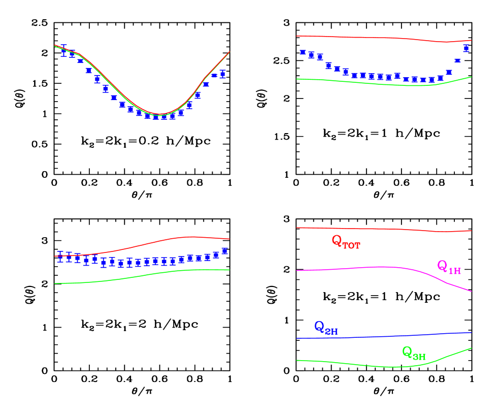
Figure 4: Comparison of the N-body results with the predictions of halo models for the reduced bispectrum as a function of triangle shape. Symbols and error bars are as in Fig. 1. Solid lines show the predictions of ST (top) and PS (bottom) mass functions. The top panels and lower left panel show different scales, whereas the lower right panel shows the partial contributions to the total value, from 1-halo, 2-halo and 3-halo terms for the ST case.

There are several approximations involved in this result. First, we take the large-scale limit $M_{11}\approx 1$, $M_{21}\approx 0$, valid to a good approximation because of the consistency conditions, Eq. (22). In addition, we assume that the configuration dependence of the 1-halo and 2-halo terms in Eq.(24) can be neglected (this holds very well for the 2-halo term and approximately for the 1-halo term, as we shall discuss below; e.g. see bottom right panel in Fig. 4). We can thus evaluate these terms for equilateral configurations, and simplify the angular integration by further assuming $W_{1}W_{2}W_{12}\approx W_{1}^{2}W_{2}^{2}$, the leading-order term in the multipolar expansion. With similar approximations, we can derive higher-order connected moments. Define

$$A_{ij}(R)\equiv\int\frac{dy}{y}\tilde{n}(y)\ b_{i}(y)\ y^{3(j+1)}\ [\overline{u}(R,y)]^{j}\ \overline{u^{2}}(R,y),$$ (30)

so that $\sigma^{2}=\sigma_{L}^{2}+A_{00}$ and $\mathop{\langle}\delta^{3}\mathop{\rangle}=S_{3}^{\rm PT}\sigma^{4}_{L}+3\sigma^{2}_{L}A_{10}+A_{01}$. Then it follows that

$$\mathop{\langle}\delta^{4}\mathop{\rangle_{c}}=S_{4}^{\rm PT}\sigma^{6}_{L}+6\frac{S_{3}^{\rm PT}}{3}\sigma^{4}_{L}A_{10}+7\frac{4\sigma^{2}_{L}}{7}A_{11}+A_{02},$$ (31)

$$\mathop{\langle}\delta^{5}\mathop{\rangle_{c}}=S_{5}^{\rm PT}\sigma^{8}_{L}+10\frac{S_{4}^{\rm PT}}{16}\sigma^{6}_{L}A_{10}+25\frac{3S_{3}^{\rm PT}}{5}\sigma^{4}_{L}A_{11}+15\frac{\sigma^{2}_{L}}{3}A_{12}+A_{03},$$ (32)

where the terms in $\mathop{\langle}\delta^{n}\mathop{\rangle_{c}}$ are ordered from $n$-halo to 1-halo contributions. The coefficient of an $m$-halo contribution to $\mathop{\langle}\delta^{n}\mathop{\rangle_{c}}$ is given by $s(n,m)$ (e.g. $6$ and $7$ in the second and third terms of Eq. [31]), the Stirling number of second kind, which is the number of ways of putting $n$ distinguishable objects ($\delta$) into $m$ cells (halos), with no cells empty (Scherrer & Bertschinger 1991). Thus, in general we can write

$$\mathop{\langle}\delta^{n}\mathop{\rangle_{c}}=S_{n}^{\rm PT}\sigma^{2(n-1)}_{L}+\sum_{m=2}^{n-1}s(n,m)\ \alpha_{nm}S_{m}^{\rm PT}\ \sigma^{2(m-1)}_{L}A_{1n-m-1}+A_{0n-2},$$ (33)

where the first term in Eq. (33) represents the $n-$halo term, the second the contributions from $m$-halo terms, and the last is the 1-halo term. The coefficients $\alpha_{nm}$ measure how many of the terms contribute as $A_{1n-m-1}$, the other contributions being subdominant. For example, in Eq. (31) the 2-halo term has a total contribution of 7 terms, 4 of them contain 3 particles in one halo and 1 in the other, and 3 of them contain 2 particles in each. The factor $4/7$ is included to take into account that the $3-1$ amplitude dominates over the $2-2$ amplitude. Note that in these results we neglected all the contributions from the non-linear biasing parameters in view of the consistency conditions, Eq. (22). When neglecting halo-halo correlations, Eq.(33) reduces to those in Sheth (1996) in the limit that halos are point-size objects ($u(\hat{k},y)=1$).

For the perturbative values, we use (Bernardeau 1994)

$$S_{3}^{\rm PT}=\frac{34}{7}-\gamma,\ \ \ \ \ S_{4}^{\rm PT}=\frac{60712}{1323}-\frac{62}{3}\gamma+\frac{7}{3}\gamma^{2},$$ (34)

$$S_{5}^{\rm PT}=\frac{200575880}{305613}-\frac{1847200}{3969}\gamma+\frac{6940}{63}\gamma^{2}-\frac{235}{27}\gamma^{3},$$ (35)

where for simplicity we neglect derivatives of $\gamma$ with respect to scale, which is a good approximation for $R\mathrel{\mathchoice{\lower 3.6pt\vbox{\halign{$\mathsurround=0pt\displaystyle\hfill#\hfil$\cr<\crcr\sim\crcr}}}{\lower 3.6pt\vbox{\halign{$\mathsurround=0pt\textstyle\hfill#\hfil$\cr<\crcr\sim\crcr}}}{\lower 3.6pt\vbox{\halign{$\mathsurround=0pt\scriptstyle\hfill#\hfil$\cr<\crcr\sim\crcr}}}{\lower 3.6pt\vbox{\halign{$\mathsurround=0pt\scriptscriptstyle\hfill#\hfil$\cr<\crcr\sim\crcr}}}}20$ Mpc/h.

Before we compare these predictions for dark matter clustering with numerical simulations, it is important to note that, within this framework, there are many ingredients which can be adjusted to improve agreement with simulations. Rather than exploring all possible variations, we have chosen to always use the NFW halo profile and the dependence of the concentration parameter on mass given earlier, and only change the mass function between PS and ST; it turns out that these two models usually bracket the results of numerical simulations. Other choices are considered in Seljak (2000), Ma & Fry (2000), Cooray & Hu (2000). The sensitivity of the results to these choices reflects the underlying uncertainty in this type of calculation. As numerical simulation results converge on the different ingredients, however, the predictive power of this method will increase.

3 Comparison with Numerical Simulations

We have run two sets of N-body simulations using the adaptive P³M code Hydra (Couchman, Thomas, & Pearce 1995). Both have $128^{3}$ particles and correspond to a $\Lambda$CDM model ($\Omega=0.3$, $\Omega_{\Lambda}=0.7$) with $\sigma_{8}=0.9$. The first set contains 14 realizations of a box-size 100 Mpc/h, and softening length $l_{\rm soft}=100$ kpc/h. The second set has 4 realizations of a box-size 300 Mpc/h, and $l_{\rm soft}=250$ kpc/h, which allows us to check for finite volume effects. We have also studied the effects of changing the softening, number of time-steps and $\Omega$ as described below.

3.1 Bispectrum Measurements: Finite Volume Effects

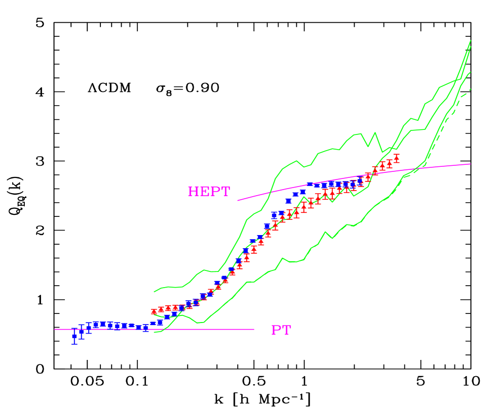
Figure 1: The reduced bispectrum $Q_{\rm eq}(k)$ for equilateral configurations as a function of scale. The triangle symbols show the average over 14 realizations of box size $L_{\rm box}=100$ Mpc/h; the 3 solid lines represent results for 3 individual realizations. The dashed line denotes the same realization as the companion solid line but ran with half the softening length (50 Kpc/h). The square symbols denote the average over 4 realizations with $L_{\rm box}=300$ Mpc/h. The disagreement of the large and small box measurements is due to finite-volume effects in the latter.

Figure 1 shows the results on the reduced bispectrum for equilateral triangles as a function of scale. The square symbols show the measurements from the “large” box ($L_{\rm box}=300$ Mpc/h) whereas the triangle symbols show the measurements from the “small” box ($L_{\rm box}=100$ Mpc/h). Error bars are obtained from the scatter among 4 and 14 realizations, respectively. The disagreement between the results of the large and small boxes is a result of finite volume effects; the bispectrum is much more sensitive to the presence or absence of massive halos than the power spectrum (we will quantify this below), so the smallness of the small box is important. Note that the total volume in the 14 small-box realizations only adds up to about half of the volume of a single large-box realization. This translates into a large scatter among realizations of the small box; 3 such realizations are shown as solid lines in Fig. 1. Note that not only the amplitude of $Q_{\rm eq}$ but also its dependence on scale fluctuates significantly from realization to realization, so one must interpret measurements made using only a small number of small volume simulations very cautiously. A similar situation holds for higher-order moments (e.g. Colombi, Bouchet & Hernquist 1996), as we shall see below.

As is well known, the distribution of higher-order statistics is non-Gaussian with positive skewness (e.g. Szapudi & Colombi 1996; Szapudi et al. 1999); the mean value of a higher-order statistic is a consequence of having a few large excursions above the mean, with most values underestimating the mean. This is exactly what we see in the small box realizations: most of them are closer to the bottom solid line than the top one in Fig. 1. Even fourteen realizations of the small box are not enough to recover the correct answer given by the large-box mean (square symbols). In other words, the skewness of the $Q$ distribution makes convergence towards the true value much slower for the small-box simulations (Szapudi & Colombi 1996; see also Scoccimarro 2000 for the bispectrum case). Notice that this is not bias in a statistical sense: given sufficient number of realizations, the mean will always converge to the true value; it is just that the convergence is slow. It is also important to note that when measuring $Q$ from multiple realizations, one should always obtain the average of $B$ and the average of $P$ separately from the realizations, and only at the end divide to obtain $Q$ (which is what we have done in making Fig. 1). Otherwise, a “ratio” bias would result (Hui & Gaztañaga 1999), and the skewness measurements from the small box simulations would be lower than are shown in Fig. 1. Such an estimator bias will certainly affect measurements of $Q$ from, say, a single realization of a size similar to our small box.

Figure 1 also shows the predictions of (tree-level) PT, which agree very well with the large-box results at large scales, as well as the predictions of hyperextended PT (HEPT; Scoccimarro & Frieman 1999), which has been proposed as a description of clustering in the non-linear regime ($k\mathrel{\mathchoice{\lower 3.6pt\vbox{\halign{$\mathsurround=0pt\displaystyle\hfill#\hfil$\cr>\crcr\sim\crcr}}}{\lower 3.6pt\vbox{\halign{$\mathsurround=0pt\textstyle\hfill#\hfil$\cr>\crcr\sim\crcr}}}{\lower 3.6pt\vbox{\halign{$\mathsurround=0pt\scriptstyle\hfill#\hfil$\cr>\crcr\sim\crcr}}}{\lower 3.6pt\vbox{\halign{$\mathsurround=0pt\scriptscriptstyle\hfill#\hfil$\cr>\crcr\sim\crcr}}}}1$ h/Mpc). The agreement with HEPT is good up to the resolution scale of our simulations, which we estimate as $k\approx 4$ h/Mpc. It is not straightforward to assign a resolution scale in Fourier space (i.e. it is not just $2\pi/l_{\rm soft}$, since a given Fourier mode has contribution from a range of scales. Two-body relaxation causes the two-point correlation function to be underestimated at scales comparable to $l_{\rm soft}$, which in turn implies an overestimate of the reduced bispectrum $Q$. To illustrate this, we have run the same realization after halving $l_{\rm soft}$ to $50$ Kpc/h (dashed line in Fig. 1); this shows that beyond $k\approx 4$ h/Mpc the bispectrum results are sensitive to the resolution, so we only plot the small-box results up to this scale. Similarly, we only show results for the large box up to $k\approx 2$ h/Mpc. For our particle number, $l_{\rm soft}$ cannot be pushed too much smaller than the values we used, else there would be not enough particles in a cell of radius $l_{\rm soft}$ to satisfy the fluid limit. We have also checked the sensitivity of our results to changes in the number of time steps used in the N-body integrator and found no difference. Changing the density parameter $\Omega$ leads to extremely small differences in the reduced bispectrum $Q$, we thus present results only for $\Lambda$CDM. This is true not only in the weakly non-linear regime, but also in the non-linear regime, as expected from the general nature of the $\Omega$ dependence in the equations of motion (Scoccimarro et al. 1998).

Recently Ma & Fry (2000) claimed that the hierarchical ansatz is not obeyed in N-body simulations. They based their claim on analysis of one single realization—the equivalent to just one of our small boxes. Their measurement approximately follows the lower solid line in Fig. 1, which, as we have shown, is seriously affected by finite volume effects (we will quantify these effects shortly). To reliably test the hierarchical ansatz at smaller scales than probed here, one must resort to higher resolution simulations, preferably keeping the box size as large as possible to avoid finite volume effects. For example, a 300 Mpc/h box $512^{3}$ particle simulation would be able to probe up to $k\approx 10$ h/Mpc reliably.

3.2 Comparison with Predictions

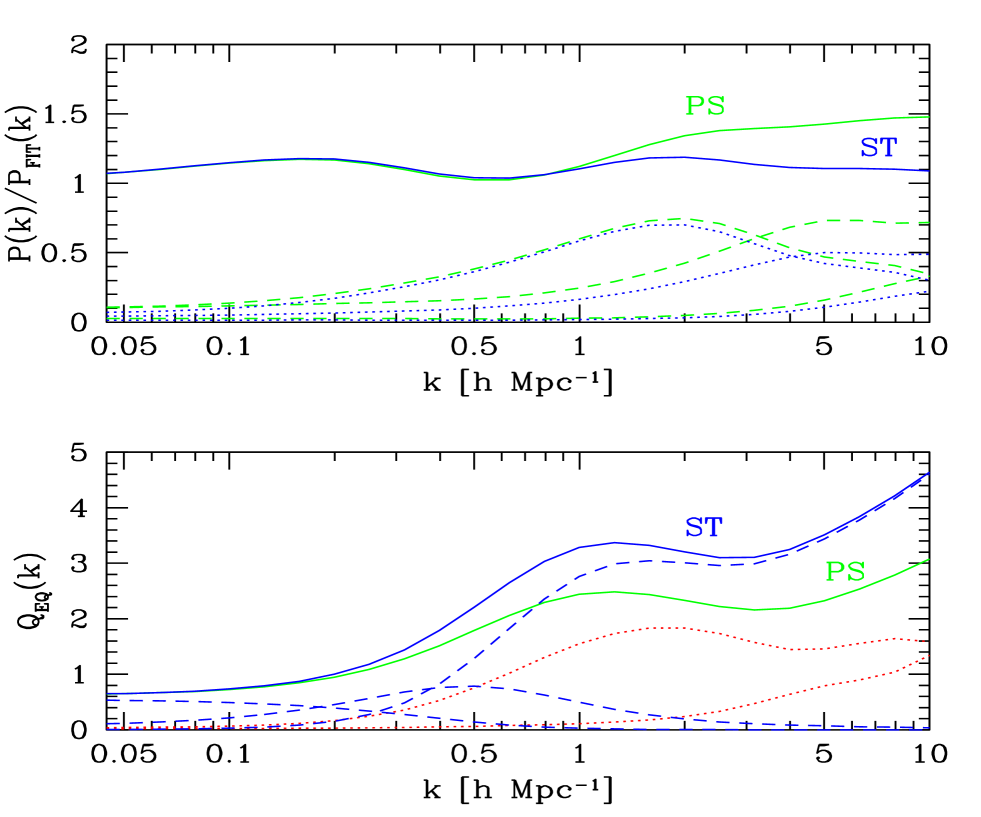
Figure 2: The top panel shows the ratio of power spectra for the PS and ST mass function to the fitting formula for the non-linear power spectrum of Peacock & Dodds (1996) as a function of scale. The dashed (dotted) lines show the contributions to the 1-halo term in the PS (ST) case from halos of mass $10<m/m_{*}<100$, $1<m/m_{*}<10$ and $0.1<m/m_{*}<1$ from left to right. Bottom panel shows the predictions for the reduced equilateral bispectrum; the dashed lines show the individual contributions (for the ST case) of 3-halo, 2-halo and 1-halo terms, which dominate at large, intermediate and small scales, respectively. The dotted lines show the contributions to the 1-halo term in $Q$ in the PS case from halos in the mass range $10<m/m_{*}<100$ and $1<m/m_{*}<10$.

The top panel in Fig. 2 shows the ratio of the power spectrum in our two models (PS and ST mass functions) to the power spectrum fitting formula (Hamilton et al. 1991; Jain, Mo & White 1995; Peacock & Dodds 1996) as a function of scale $k$. The dashed (dotted) lines show the contributions to the 1-halo term in the PS (ST) case from halos having masses in the range $10<m/m_{*}<100$, $1<m/m_{*}<10$, and $0.1<m/m_{*}<1$, from left to right ($m_{*}=1.07\times 10^{13}M_{\sun}$/h). As the PS mass function has more halos than the ST one when $m\mathrel{\mathchoice{\lower 3.6pt\vbox{\halign{$\mathsurround=0pt\displaystyle\hfill#\hfil$\cr<\crcr\sim\crcr}}}{\lower 3.6pt\vbox{\halign{$\mathsurround=0pt\textstyle\hfill#\hfil$\cr<\crcr\sim\crcr}}}{\lower 3.6pt\vbox{\halign{$\mathsurround=0pt\scriptstyle\hfill#\hfil$\cr<\crcr\sim\crcr}}}{\lower 3.6pt\vbox{\halign{$\mathsurround=0pt\scriptscriptstyle\hfill#\hfil$\cr<\crcr\sim\crcr}}}}40m_{*}$, the 1-halo term is enhanced. Note the dip in both predictions at $k\approx 0.5$ h/Mpc, where the amplitude of 1-halo and 2-halo terms are comparable. This is due to our treatment of the 2-halo term; we approximate it by simply using linear PT. In practice, non-linear corrections enhance this term at scales smaller than the non-linear scale, $k\approx 0.3$ h/Mpc. However, when including this term one must also take into account exclusion effects (halos cannot be closer than their typical size), otherwise the power spectrum at intermediate scales would be overestimated. Since exclusion effects are non-trivial to compute (though Sheth & Lemson 1999 suggest how one might do so), the simplest solution is to ignore these effects, because they approximately cancel each other. This is a reasonable approximation because at the scales where exclusion effects become important, 1-halo contributions dominate.

The bottom panel in Fig. 2 shows the prediction of halo models for the reduced bispectrum for equilateral configurations as a function of scale (solid lines). For the ST case we also show the partial contributions from 1-halo, 2-halo and 3-halo terms in dashed lines, which dominate at small, intermediate and large scales, respectively. For the PS case we show in dotted lines the contributions to the 1-halo term in $Q$ when the bispectrum is restricted to the mass range $10<m/m_{*}<100$ (which dominates at all scales shown in the plot) and $1<m/m_{*}<10$. In this case, when taking the ratio in Eq. (26), we have used the full power spectrum. As expected, comparing the two panels we see that at a given scale the bispectrum is dominated by larger mass halos than the power spectrum. For the bispectrum at $k\approx 1$h/Mpc, this implies that halos with $m>40m_{*}$ contribute more significantly, thus leading to a higher $Q$. At smaller scales, say $k\approx 10$h/Mpc, the PS mass function has more halos of the relevant masses ($m<40m_{*}$), so the bispectrum is larger for PS than ST (by a factor slightly smaller than the ratio of power spectra), thus the reduced bispectrum $Q$ is higher again for the ST case. We have also varied the concentration parameter to test the sensitivity of our results. Doubling the concentration parameter (with the same mass dependence) leads to a significant increase of the power spectrum at small scales (this consistent with Seljak 2000) and increases $Q$ by about 10% at small scales. On the other hand, changing the scaling of the concentration parameter by a factor of two to $c(m)=9(m/m_{*})^{-0.26}$, decreases (increases) the power spectrum at scales where $m/m_{*}>1$ ($m/m_{*}<1$) contributes, as expected. For the bispectrum, larger concentration leads to higher $Q$, although at a given scale larger masses contribute than for the power spectrum, so the effects are shifted in scale with respect to the power spectrum case.

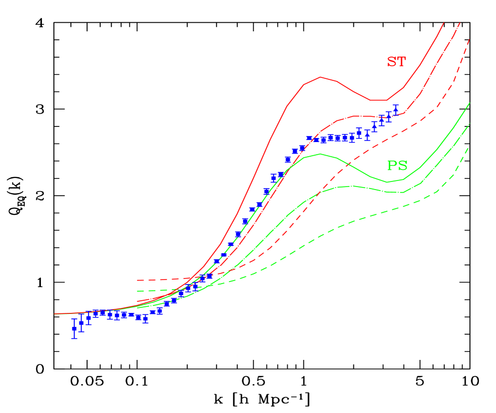
Figure 3: Comparison of the N-body results of Fig. 1 (points with error-bars) with the predictions of Fig. 2 (solid lines). The dashed lines show the predictions of halo models when there are no halos of mass larger than $m=10^{14}~{}M_{\sun}$/h in the simulation volume, to illustrate finite volume effects, for both PS (lower curve) and ST mass functions. The dot-dashed lines represent the predictions if halos of mass larger than $m=5.9\times 10^{14}M_{\sun}/h$ (or $m=6.8\times 10^{14}M_{\sun}/h$) are excluded for PS (or ST) mass functions.

Figure 3 compares these results with the measurements in the numerical simulations presented in Fig. 1. We see that generally there is good agreement between predictions and the simulations; the simulations seem to be roughly in between the PS and ST predictions. At small scales, the halo models predict that $Q_{eq}$ increases rapidly with $k$; the limited resolution of our simulations prevents us from testing this particular prediction reliably. As we discussed above, finite volume effects can be significant when dealing with the bispectrum. To quantify this, we have calculated the halo model predictions for cases when the maximum halo mass is set to $m_{\rm max}=5.9\times 10^{14}M_{\sun}$/h and $m_{\rm max}=6.8\times 10^{14}M_{\sun}$/h for PS and ST respectively (dot-dashed lines) and $m_{\rm max}=10^{14}M_{\sun}$/h (dashed lines). These values are those for which the mass functions would predict just one halo with mass larger than $m_{\rm max}$ in a $(100{\rm Mpc/h})^{3}$ volume; but since these are cumulative numbers and both mass functions actually overestimate the number of halos when compared to simulations (more so PS), a smaller number, such as $m_{\rm max}=10^{14}M_{\sun}$/h is perhaps a more reasonable cutoff. In any case, we see that the predictions change significantly; in particular, introducing such a cutoff makes the scale dependence of $Q$ much more like that seen in most of the realizations of the small box (bottom solid line in Fig. 1).

One key element in the halo model is that we are using the spherical average (rather than the actual shapes) of halo profiles. On the other hand, it is well known that halos found in N-body simulations are not spherical, but rather triaxial (Barnes & Efstathiou 1987; Frenk et al. 1988; Zurek, Quinn & Salmon 1988). The bispectrum is the lowest-order statistic which is sensitive to the shapes of structures, so one expects to find differences for the bispectrum as a function of triangle shape at small scales where halo profiles (1-halo terms) determine correlation functions. Figure 4 shows such a comparison at different scales, for triangles where $k_{2}=2k_{1}$, as a function of angle $\theta$ between ${\hbox{\BF k}}_{1}$ and ${\hbox{\BF k}}_{2}$. The top left panel shows that, at large scales, the bispectrum agrees reasonably well with simulations; this is of course by construction, since non-linear PT holds. At smaller scales (top right panel), however, the predictions become independent of triangle shape at scales where there is still noticeable configuration dependence. In fact, this is understood from the bottom right panel which shows the partial contributions for the ST case. We see that the 1-halo term (which is determined by the halo profiles) has the opposite configuration dependence than the 3-halo term, which comes from non-linear PT.

The fact that $Q_{1h}$ is convex can be understood from the spherical approximation. If halos were exactly spherical and $Q$ were scale-independent, then one would expect the maximum of $Q$ to occur for equilateral configurations. When $k_{2}=2k_{1}$ the closest configurations to equilaterals are isosceles triangles with $\theta\approx 0.6\pi$. Aside from an overall slight scale dependence ($\theta=0$ configurations are somewhat more non-linear than $\theta=\pi$), we see that this is indeed the case. Notice also that, if the contribution $Q_{1h}$ were flat, the residual configuration coming from $Q_{3h}$ would be enough to produce agreement with the N-body simulations. At even smaller scales (bottom left panel), the numerical simulation results become approximately flat, but the halo models predict a convex configuration dependence due to the fact that $Q_{1h}$ dominates. From these results we conclude that although halo models predict bispectrum amplitudes which are in reasonable agreement with simulations, the configuration dependence is in qualitative disagreement with simulations. Of course, if we knew the actual halo shapes, then they could be incorporated into the models (at the expense of complicating the calculations!).

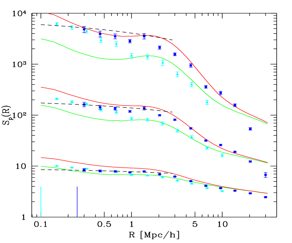
Figure 5: $S_{p}$ parameters ($p=3,4,5$ from bottom to top) as a function of smoothing scale $R$. Symbols and error bars are as in Fig. 1. Solid lines show the predictions of ST (upper) and PS (lower) mass functions. Dashed lines show the asymptotic behavior predicted by HEPT. Again, the disagreement of the small volume simulations (triangles) with those of bigger volume (squares) is a direct consequence of finite volume effects in the former. The vertical lines denote the softening length of the two sets of simulations.

Finally, in Fig. 5, we compare counts-in-cells measurements of the higher-order moments of the smoothed density field in our simulations with the predictions of halo models. Symbols and error bars are as in Fig.1: the top (bottom) solid line in each case corresponds to the ST (PS) prediction. The dashed lines show the predictions of HEPT (Scoccimarro & Frieman 1999), and the vertical lines show the softening scale of the large and small box. The disagreement of the average of 14 small-box measurements with the large-box average is, again, a manifestation of finite volume effects. As expected, the difference becomes increasingly important for the higher order moments. Despite the many approximations made in the calculations of $S_{p}$ parameters in halo models, the agreement with simulations is quite good. We also see a very good agreement with the HEPT predictions, and that the scales where halo models predict a strong scale dependence are beyond the limits of our resolution. This also confirms that our prescription for the resolution limit in Fourier space was reasonably accurate. Thus, contrary to Ma & Fry (2000), we conclude that higher-resolution simulations in bigger boxes are essential if one is to test models of the higher-order correlations reliably.

4 Galaxy Clustering

We now turn to a discussion of how to use the halo models described above to predict the clustering of galaxies. Our treatment follows ideas present in the semianalytic galaxy formation models (Benson et al. 2000; Kauffmann et al. 1999) and has been also explored by Seljak (2000) and Peacock & Smith (2000) for the case of the power spectrum.

4.1 Galaxy Correlation Functions

To describe galaxy clustering, we need to know the distribution, the mean and the higher-order moments, of the number of galaxies which can inhabit a halo of mass $m$. In addition, we need to know the spatial distribution of galaxies within their parent halo. To illustrate our model predictions, in what follows we will assume that the galaxies follow the dark matter profile (we will discuss what happens if we change this requirement shortly). This implies that Eq. (7) for galaxies reads

$$\bar{n}_{g}^{2}P_{g}(k) = (2\pi)^{3}\int n(m)\mathop{\langle}N_{\rm gal}^{2}(m)\mathop{\rangle}dm|u_{m}({\hbox{\BF k}})|^{2}+$$ (36)

$$(2\pi)^{6}\int u_{m_{1}}(k)n(m_{1})\mathop{\langle}N_{\rm gal}(m_{1})\mathop{\rangle}dm_{1}\int u_{m_{2}}(k)n(m_{2})\mathop{\langle}N_{\rm gal}(m_{2})\mathop{\rangle}dm_{2}P(k;m_{1},m_{2}),$$

where the mean number density of galaxies is

$$\bar{n}_{g}=\int n(m)\mathop{\langle}N_{\rm gal}(m)\mathop{\rangle}dm.$$ (37)

Thus, knowledge of the number of galaxies per halo moments $\mathop{\langle}N_{\rm gal}^{n}(m)\mathop{\rangle}$ as a function of halo mass gives a complete description of the galaxy clustering statistics within this framework. Note that when the mean number of galaxies per halo drops below unity, one must use $u_{m}({\hbox{\BF k}})=1$, the point-size halo limit, since in this case there is at most a single galaxy (which we assume to be at the center of the halo).

The results for galaxy power spectrum and bispectrum follow those of the dark matter in Eqs.(23-24), after changing $M_{ij}$ in Eq. (25) to $G_{ij}$, where

$$G_{ij}(\hat{k}_{1},\ldots,\hat{k}_{j})\equiv\frac{1}{\bar{n}_{g}^{j}}\int\frac{dy}{y}\tilde{n}(y)b_{i}(y)[u(\hat{k}_{1},y)\ldots u(\hat{k}_{j},y)]\Big{(}\frac{R_{*}^{3}y^{3}}{6\pi^{2}}\Big{)}^{j-1}\frac{\mathop{\langle}N_{\rm gal}^{j}\mathop{\rangle_{c}}}{m^{j}}.$$ (38)

Note that in the large-scale limit, the galaxy bias parameters are

$$b_{i}=G_{i1}\approx\frac{1}{\bar{n}_{g}}\int\frac{dy}{y}\tilde{n}(y)b_{i}(y)\frac{\mathop{\langle}N_{\rm gal}\mathop{\rangle}}{m}.$$ (39)

Similarly, the galaxy one-point connected moments satisfy

$$\sigma_{g}^{2}=(\sigma^{2}_{L})_{\rm gal}+B_{00},\ \ \ \ \ \mathop{\langle}\delta_{g}^{3}\mathop{\rangle_{c}}=(S_{3}^{\rm PT})_{\rm gal}(\sigma^{4}_{L})_{\rm gal}+3(\sigma^{2}_{L})_{\rm gal}B_{10}+B_{01},$$ (40)

$$\mathop{\langle}\delta_{g}^{4}\mathop{\rangle_{c}}=(S_{4}^{\rm PT})_{\rm gal}(\sigma^{6}_{L})_{\rm gal}+2S_{3}^{\rm hh}(\sigma^{4}_{L})_{\rm gal}B_{10}+4(\sigma^{2}_{L})_{\rm gal}B_{11}+B_{02},$$ (41)

and

$$\mathop{\langle}\delta_{g}^{5}\mathop{\rangle_{c}}=(S_{5}^{\rm PT})_{\rm gal}(\sigma^{8}_{L})_{\rm gal}+\frac{5}{8}S_{4}^{\rm hh}(\sigma^{6}_{L})_{\rm gal}B_{10}+15S_{3}^{\rm hh}(\sigma^{4}_{L})_{\rm gal}B_{11}+5(\sigma^{2}_{L})_{\rm gal}B_{12}+B_{03},$$ (42)

where

$$B_{ij}(R)\equiv\frac{1}{b_{i}\bar{n}_{g}^{j+2}}\int\frac{dy}{y}\tilde{n}(y)\ b_{i}(y)\ y^{3(j+1)}\ [\overline{u}(R,y)]^{j}\ \overline{u^{2}}(R,y)\frac{\mathop{\langle}N_{\rm gal}^{j+2}\mathop{\rangle}}{m^{j+2}},$$ (43)

and the perturbative moments are given by their local bias counterparts (Fry & Gaztañaga 1993)

$$(\sigma^{2}_{L})_{\rm gal}=b_{1}^{2}\sigma^{2}_{L},\ \ \ \ \ (S_{3}^{\rm PT})_{\rm gal}=\frac{1}{b_{1}}\Big{(}S_{3}^{\rm PT}+3c_{2}\Big{)},\ \ \ \ \ (S_{4}^{\rm PT})_{\rm gal}=\frac{1}{b_{1}^{2}}\Big{(}S_{4}^{\rm PT}+12c_{2}S_{3}^{\rm PT}+4c_{3}+12c_{2}^{2}\Big{)},$$ (44)

and

$$(S_{5}^{\rm PT})_{\rm gal}=\frac{1}{b_{1}^{3}}\Big{(}S_{5}^{\rm PT}+20c_{2}S_{4}^{\rm PT}+15c_{2}(S_{3}^{\rm PT})^{2}+(30c_{3}+120c_{2}^{2})S_{3}^{\rm PT}+5c_{4}+60c_{2}c_{3}+60c_{2}^{3}\Big{)},$$ (45)

where $c_{i}\equiv b_{i}/b_{1}$ and $b_{i}$ are the effective bias parameters in Eq. (39). The halo-halo skewness and kurtosis are given by these expressions upon replacing $c_{i}$ by $c_{i}B_{i0}/B_{10}$.

4.2 Galaxies

As a first example, we use the results of the semi-analytic models of Kauffmann et al. (1999); these N-body simulations, halo and galaxy catalogues are publically available. Sheth & Diaferio (2000) show that in these catalogues, the mean number of galaxies $N_{\rm gal}$ per halo of mass $m$ are well fit by

$$\mathop{\langle}N_{\rm gal}\mathop{\rangle}=\mathop{\langle}N_{B}+N_{R}\mathop{\rangle},\ \ \ \ \ \mathop{\langle}N_{B}\mathop{\rangle}=0.7(m/m_{B})^{\alpha_{B}},\ \ \ \ \ \mathop{\langle}N_{R}\mathop{\rangle}=(m/m_{R})^{\alpha_{R}},$$ (46)

where $N_{B}$ and $N_{R}$ represent the number of blue and red galaxies per halo of mass $m$, and $\alpha_{B}=0$ for $10^{11}M_{\sun}/h\leq m\leq m_{B}$, $\alpha_{B}=0.8$ for $m>m_{B}$, $m_{B}=4\times 10^{12}M_{\sun}/h$, $\alpha_{R}=0.9$, and $m_{R}=2.5\times 10^{12}M_{\sun}/h$ (no lower mass cut-off for $R$). The physical basis for this relation is as follows. At large masses, the gas cooling time becomes larger than the Hubble time, so galaxy formation is suppressed in large-mass halos, therefore $\mathop{\langle}N_{\rm gal}\mathop{\rangle}$ increases less rapidly than the mass. In small-mass halos, however, effects such as supernova winds can blow away the gas from halos, also suppressing galaxy formation, thus the cutoff at small masses.

To calculate the power spectrum and higher-order statistics we also need the second and higher-order moments of $N_{\rm gal}$. The second moment is also obtained from the semi-analytic models, and obeys

$$\mathop{\langle}N_{\rm gal}(N_{\rm gal}-1)\mathop{\rangle}\equiv\alpha^{2}(m)\mathop{\langle}N_{\rm gal}\mathop{\rangle}^{2},$$ (47)

where the function $\alpha(m)$ quantifies deviations from Poisson statistics $\alpha(m)\approx\log\sqrt{m/m_{11}}$ ($m_{11}\equiv 10^{11}M_{\sun}/h$) for $m<10^{13}M_{\sun}/h$ and $\alpha(m)=1$ otherwise; that is, for large masses the scatter about the mean number of galaxies is Poisson, whereas for small masses it is sub-Poisson.

To model the higher-order moments we will assume that the number of galaxies in a halo of mass $m$ follows a binomial distribution:

$$p(N_{\rm gal}=n|m)={{\cal N}_{m}\choose n}p_{m}^{n}(1-p_{m})^{{\cal N}_{m}-n}.$$ (48)

The binomial distribution is characterized by two parameters, ${\cal N}_{m}$ and $p_{m}$, which we set by requiring that the first two moments of the distribution equal those from the semianalytics. Specifically, the first and second factorial moments are ${\cal N}_{m}p_{m}$ and ${\cal N}_{m}p_{m}({\cal N}_{m}p_{m}-p_{m})$, and we require that they equal $\mathop{\langle}N_{\rm gal}\mathop{\rangle}$ and $\mathop{\langle}N_{\rm gal}(N_{\rm gal}-1)\mathop{\rangle}$, respectively. One can think of ${\cal N}_{m}$ as the maximum number of galaxies which can be formed with the available mass $m$, and of $p_{m}$ as the probability of actually forming a galaxy. For a constant ${\cal N}_{m}p_{m}$, the small $p_{m}$ limit gives a Poisson distribution. ${\cal N}_{m}$ is an increasing function of mass, whereas $p_{m}$ peaks at $m\approx 10^{12}M_{\sun}/h$ with $p_{m}\approx 0.8$. The higher-order factorial moments are completely determined once the first two moments have been specified; they obey

$$\mathop{\langle}N_{\rm gal}(N_{\rm gal}-1)\ldots(N_{\rm gal}-j)\mathop{\rangle}=\alpha^{2}(2\alpha^{2}-1)\ldots(j\alpha^{2}-j+1)\mathop{\langle}N_{\rm gal}\mathop{\rangle}^{j+1}.$$ (49)

In this model, all the moments become Poisson-like at the same mass scale, i.e. when $\alpha(m)=1$, all the factorial moments become Poisson, $\mathop{\langle}N_{\rm gal}(N_{\rm gal}-1)\ldots(N_{\rm gal}-j)\mathop{\rangle}=\mathop{\langle}N_{\rm gal}\mathop{\rangle}^{j+1}$. However, at small scales, where small halos contribute, the galaxy counts per halo are significantly sub-Poisson. Our binomial model provides a simple way of accounting for this. To correct the power spectrum and bispectrum for shot noise we use the same form as in the Poisson case (Peebles 1980):

$$P^{\rm c}(k)=P(k)-\varepsilon,\ \ \ \ \ B_{123}^{\rm c}=B_{123}-\varepsilon(P_{1}^{\rm c}+P_{2}^{\rm c}+P_{3}^{\rm c})-\varepsilon^{2},$$ (50)

but where the parameter $\varepsilon$ is set to $\varepsilon\equiv P(k\rightarrow\infty)$, to avoid making the corrected power spectrum negative at small scales. In the Poisson case, $\varepsilon^{-1}=(2\pi)^{3}\bar{n}_{g}$, we find that in our prescription $\varepsilon$ can be smaller than the Poisson value by almost a factor of two. Although this model is somewhat arbitrary, our results are insensitive to shot noise substraction for $k\mathrel{\mathchoice{\lower 3.6pt\vbox{\halign{$\mathsurround=0pt\displaystyle\hfill#\hfil$\cr<\crcr\sim\crcr}}}{\lower 3.6pt\vbox{\halign{$\mathsurround=0pt\textstyle\hfill#\hfil$\cr<\crcr\sim\crcr}}}{\lower 3.6pt\vbox{\halign{$\mathsurround=0pt\scriptstyle\hfill#\hfil$\cr<\crcr\sim\crcr}}}{\lower 3.6pt\vbox{\halign{$\mathsurround=0pt\scriptscriptstyle\hfill#\hfil$\cr<\crcr\sim\crcr}}}}5$h/Mpc and smoothing scales $R\mathrel{\mathchoice{\lower 3.6pt\vbox{\halign{$\mathsurround=0pt\displaystyle\hfill#\hfil$\cr>\crcr\sim\crcr}}}{\lower 3.6pt\vbox{\halign{$\mathsurround=0pt\textstyle\hfill#\hfil$\cr>\crcr\sim\crcr}}}{\lower 3.6pt\vbox{\halign{$\mathsurround=0pt\scriptstyle\hfill#\hfil$\cr>\crcr\sim\crcr}}}{\lower 3.6pt\vbox{\halign{$\mathsurround=0pt\scriptscriptstyle\hfill#\hfil$\cr>\crcr\sim\crcr}}}}1$Mpc/h.

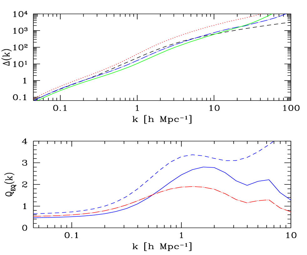
Figure 6: The top panel shows the galaxy power spectrum ($\Delta(k)=4\pi k^{3}P(k)$) as a function of scale predicted by halo models for ST (dot-dashed) and PS (solid) mass functions, using the $N_{\rm gal}(m)$ given in Eq. (46). The dashed line shows the mass power spectrum predicted by the fitting formula for the ST case. The dotted line shows the power for the ST case if the lower mass cut-off is changed from $m_{\rm cut}=10^{11}M_{\sun}/h$ to $m_{\rm cut}=10^{11.5}M_{\sun}/h$. The bottom panel shows the reduced galaxy bispectrum for equilateral triangles as a function of scale for $m_{\rm cut}=10^{11}M_{\sun}/h$ (solid), $m_{\rm cut}=10^{11.5}M_{\sun}/h$ (dot-dashed), and for the mass (dashed). These assume the ST mass function.

Figure 6 shows the resulting galaxy correlation functions. The top panel shows the predictions of the ST (dot-dashed) and PS (solid) mass functions for galaxies using the relations given above. For comparison, we also show the mass power spectrum predicted by the fitting formula of Peacock & Dodds (1996). Note how the galaxy power spectrum is well approximated by a power law, even though the dark matter spectrum is not. This is due to the fact that galaxy formation is inefficient in massive halos; this suppresses the 1-halo term compared to the dark matter case. In addition, at small scales the sub-Poisson statistics of galaxy counts per halo suppresses the galaxy spectrum relative to the dark matter. The dotted line in the top panel shows how the predictions change for the ST model when the low-mass cutoff in the $N_{\rm gal}(m)$ relation is raised from $m_{\rm cut}=10^{11}M_{\sun}$/h to $m_{\rm cut}=10^{11.5}M_{\sun}$/h. At large scales, suppressing low-mass halos leads to an increase of the bias factor from $b_{1}=0.86$ to $b_{1}=1.12$. At small scales, since these low-masses do not contribute significantly, the overall amplification of the 1-halo term is due to the lower galaxy number density, which decreases by almost a factor of two. Therefore, our galaxy clustering predictions are quite sensitive to the low-mass cutoff for galaxy formation.

The bottom panel in Fig. 6 shows the galaxy reduced bispectrum $Q_{\rm gal}$ for equilateral configurations as a function of scale (solid lines), compared to the dark matter value (dashed) for the ST mass function. At large scales, the halo models predict a negative quadratic bias, which suppresses the bispectrum. At smaller scales, both the power spectrum and bispectrum are suppressed, but at a given scale the bispectrum is sensitive to larger mass halos than the power spectrum, so $Q_{\rm gal}$ rises more gradually than $Q_{\rm dm}$. At small scales $k\mathrel{\mathchoice{\lower 3.6pt\vbox{\halign{$\mathsurround=0pt\displaystyle\hfill#\hfil$\cr>\crcr\sim\crcr}}}{\lower 3.6pt\vbox{\halign{$\mathsurround=0pt\textstyle\hfill#\hfil$\cr>\crcr\sim\crcr}}}{\lower 3.6pt\vbox{\halign{$\mathsurround=0pt\scriptstyle\hfill#\hfil$\cr>\crcr\sim\crcr}}}{\lower 3.6pt\vbox{\halign{$\mathsurround=0pt\scriptscriptstyle\hfill#\hfil$\cr>\crcr\sim\crcr}}}}1$h/Mpc, the different mass weighing of the galaxy bispectrum leads to a suppression of the scale dependence of $Q$. The dot-dashed curve shows again the sensitivity to the low-mass cutoff ($m_{\rm cut}=10^{11.5}M_{\sun}$/h); as expected, the distribution at small scales is more biased. To be more quantitative, let’s note that at small scales, where 1-halo terms dominate, the scaling of the $p$-point spectrum is

$$T_{p}(k)\sim\int n(m)\ m^{p}\ [u_{m}(k)]^{p}\ \frac{\mathop{\langle}N_{\rm gal}^{p}\mathop{\rangle}}{m^{p}}\ dm,$$ (51)

and at small masses $m\ll m_{*}$, $n(m)\sim m^{-2}\nu^{a}(m)$, $c(m)\sim m^{-b}$ and $u_{m}(k)\sim[\sin\kappa\ {\rm Sic}(\kappa)-\cos\kappa\ {\rm Ci}(\kappa)]/\ln c$, where ${\rm Sic}(\kappa)\equiv\pi/2-{\rm Si}(\kappa)$. This expression for the profile follows when $c\gg 1$, at large $\kappa$, $u_{m}(k)\sim(\kappa\ln c)^{-1}$. Furthermore, if $\nu(m)\sim m^{(n+3)/6}$ as in the scale-free case, and $\mathop{\langle}N_{\rm gal}^{p}\mathop{\rangle}\sim m^{p(1-\epsilon)}$, changing variable from $m$ to $\kappa$, we have

$$T_{p}(k)\sim k^{[6(1-p+p\epsilon)-(n+3)a]/[2(3b+1)]},$$ (52)

where we have neglected the weak logarithmic dependence of the profile on the concentration (which leads to additional suppresion at small scales) and used that the integral over $\kappa$ converges. This means that the reduced spectra $Q_{p}(k)\sim T_{p}(k)/[P(k)]^{p-1}$ scale as $Q_{p}(k)\sim k^{\gamma_{p}}$ with

$$\gamma_{p}=(p-2)\frac{a(n+3)-6\epsilon}{2(3b+1)}.$$ (53)

This generalizes the derivation in Ma & Fry (2000b) for galaxies. The validity of the hierarchical ansatz, $\gamma_{p}\approx 0$, thus depends on the low-mass behavior of the concentration parameter, mass function and $N_{\rm gal}$. For scale-free initial conditions, the validity of the hierarchical ansatz for the mass correlation functions is linked to that of stable clustering (Peebles 1980), although for higher-order correlation functions stable clustering takes a different form than the usual two-point requirement that pairwise peculiar velocities cancel the Hubble flow (Jain 1997). We see that for $p=3$ (the bispectrum), $a=0.4$ (ST mass function), $\epsilon=0.1$, $n_{\rm eff}\approx-2.5$ ($k=3$ h/Mpc), and $b=0.13$, $\gamma_{3}\approx-0.3$, which agrees approximately with the behavior of $Q_{\rm gal}$ in Fig. 6. This is only qualitative, due to the many approximations involved. On the other hand, it captures the general behavior of mass weighing, for $b>0$, supressing contributions from massive halos ($\epsilon>0$) preferentially places galaxies in more concentrated halos, thus at a given $k$ one is probing outer regions of the NFW profile compared to the mass case. Since in the outer regions $u(r)\sim r^{-3}$, $Q_{\rm gal}$ is less scale dependent than $Q$.

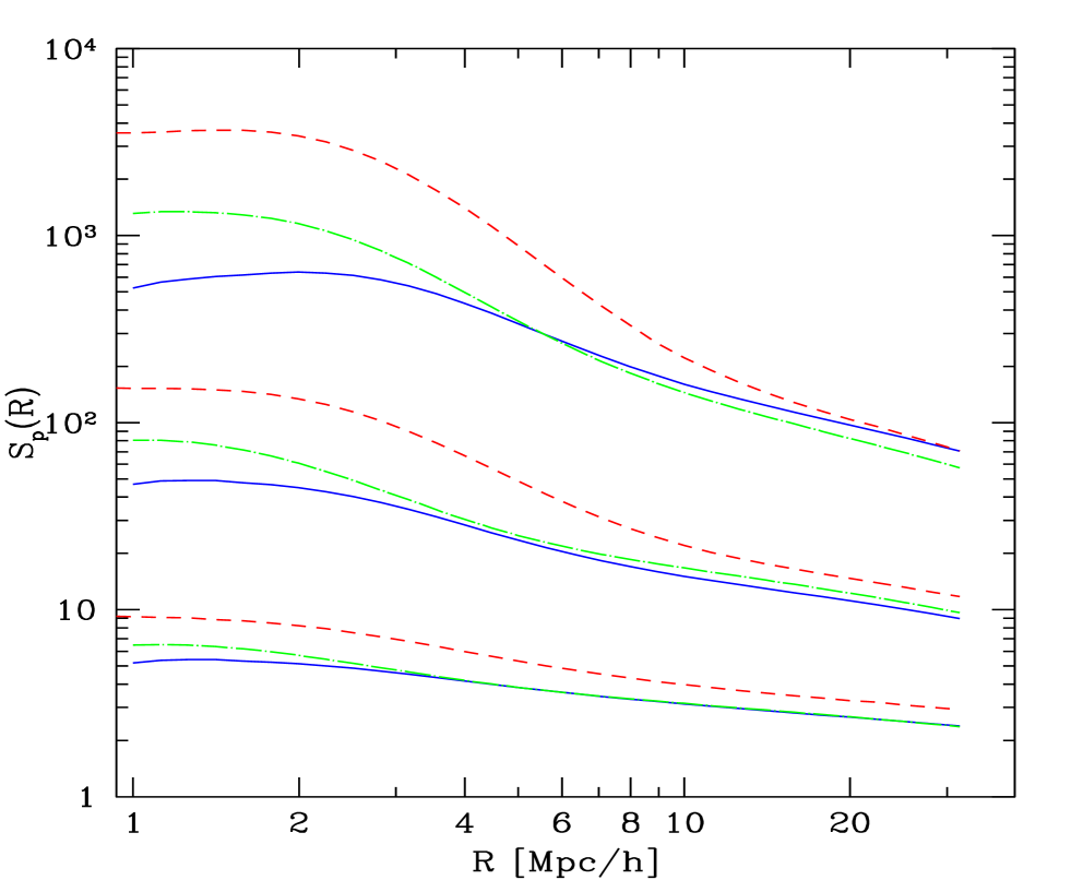
Figure 7: $S_{p}$ parameters ($p=3,4,5$ from bottom to top) as a function of smoothing scale $R$ for the mass (dashed), galaxies as in Eq.(46) with low-mass cutoff at $m_{\rm cut}=10^{11}M_{\sun}$/h (dot-dashed) and galaxies with $m_{\rm cut}=10^{11.5}M_{\sun}$/h (solid).

Figure 7 shows the $S_{p}$ parameters as a function of smoothing scale $R$ for the mass (dashed; same as ST in Fig 5), the galaxies with $m_{\rm cut}=10^{11}M_{\sun}$/h (dot-dashed) and the galaxies with $m_{\rm cut}=10^{11.5}M_{\sun}$/h (solid). Although we see the same general behavior as in the bispectrum case, it is interesting that the galaxy $S_{p}$ parameters are smaller than the dark matter ones at small scales, which is similar to the trend seen in comparisons of dark matter predictions with real galaxy catalogs. Both galaxy plots assume that the galaxy per halo moments obey Eq. (49). We have repeated the calculation assuming Poisson statistics ($\alpha(m)=1$) and found that the results are the same for scales $R\geq 5$ Mpc/h, and that at $R=1$ Mpc/h the Poisson values are about 15% below those shown in Fig. 7. The sensitivity of the clustering to the details of the relation of the number of galaxies as a function of halo mass can be used to probe aspects of galaxy formation, as we now discuss.

5 Comparison with APM Survey: Constraints on Galaxy Formation

Measurements of two-point and higher order moments of the galaxy field in the APM survey (Maddox et al. 1990) provide important constraints on models of galaxy clustering. Here we use the measurements of counts-in-cells, deprojected into three dimensions, by Gaztañaga (1994,1995) to constrain the $N_{\rm gal}(m)$ relation.

As discussed above, galaxy clustering at large scales is given by the standard local-bias model, with bias parameters obtained from Eq.(39). To constrain the $N_{\rm gal}(m)$ relation, we use the parametrized form

$$\mathop{\langle}N_{\rm gal}\mathop{\rangle}=(m/m_{0})^{a_{1}},\ \ \ \ \ m_{\rm cut}\leq m\leq m_{0},\ \ \ \ \ \ \ \ \ \ \mathop{\langle}N_{\rm gal}\mathop{\rangle}=(m/m_{0})^{a_{2}},\ \ \ \ \ m\geq m_{0},$$ (54)

with $\mathop{\langle}N_{\rm gal}\mathop{\rangle}=0$ for $m<m_{\rm cut}$ and the second moment obeys Eq. (47) with

$$\alpha(m)=\frac{\log(m/m_{\rm cut})}{\log(m_{0}/m_{\rm cut})},$$ (55)

for $m\leq m_{0}$ and $\alpha(m)=1$ for $m\geq m_{0}$. For the higher-order moments we adopt the binomial model in Eq.(49). Requiring that $p_{m}$ in the binomial model to be positive implies that $a_{1}\geq 0$. Note that in Eq. (54) we have set $\mathop{\langle}N_{\rm gal}\mathop{\rangle}=1$ at $m=m_{0}$ since clustering statistics do not depend on the overall number density of galaxies; however, constraints such as the luminosity function and the Tully-Fisher relation are sensitive to the overall amplitude of the $N_{\rm gal}(m)$ relation.

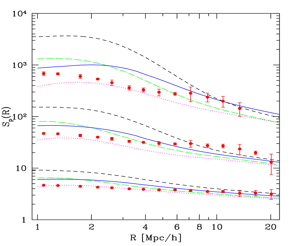
Figure 10: Same as previous figure for the $S_{p}$ parameters. In addition, the dashed lines show the predictions for the mass.

For the measured values in APM at large scales, we use that $\sigma_{g}^{2}=0.167\pm 0.021$ at $R=20$ Mpc/h, and for the higher-order moments we use $(S_{3})_{\rm gal}=3.3\pm 0.5$ and $(S_{4})_{\rm gal}=15\pm 4$ at $R=20$ Mpc/h. The latter are fiducial values obtained by averaging over the large scale ($R>10$) skewness and kurtosis, rather than the value at a particular scale. The skewness at large scales is rather flat so averaging is reasonable (see Fig. 10), for the kurtosis the large scale limit is not so well defined, but in practice this constraint is not very important because it comes with large error bars.

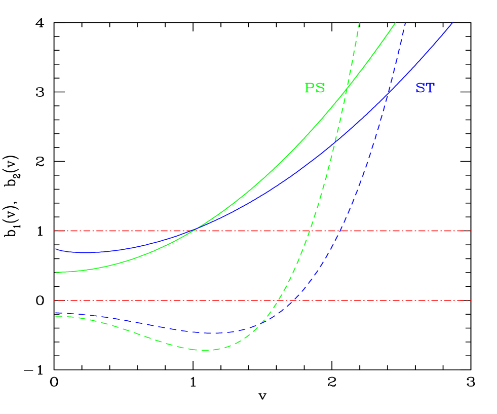
Figure 8: Halo linear ($b_{1}$, solid lines) and non-linear ($b_{2}$, dashed lines) bias parameters as a function of threshold $\nu=\delta_{c}/\sigma(m)$ for the PS and ST mass functions. The dot-dashed lines denote $b_{1}=1$ and $b_{2}=0$ for comparison.

The constraint on the variance at large scales sets the linear bias parameter, $1\mathrel{\mathchoice{\lower 3.6pt\vbox{\halign{$\mathsurround=0pt\displaystyle\hfill#\hfil$\cr<\crcr\sim\crcr}}}{\lower 3.6pt\vbox{\halign{$\mathsurround=0pt\textstyle\hfill#\hfil$\cr<\crcr\sim\crcr}}}{\lower 3.6pt\vbox{\halign{$\mathsurround=0pt\scriptstyle\hfill#\hfil$\cr<\crcr\sim\crcr}}}{\lower 3.6pt\vbox{\halign{$\mathsurround=0pt\scriptscriptstyle\hfill#\hfil$\cr<\crcr\sim\crcr}}}}b_{1}\mathrel{\mathchoice{\lower 3.6pt\vbox{\halign{$\mathsurround=0pt\displaystyle\hfill#\hfil$\cr<\crcr\sim\crcr}}}{\lower 3.6pt\vbox{\halign{$\mathsurround=0pt\textstyle\hfill#\hfil$\cr<\crcr\sim\crcr}}}{\lower 3.6pt\vbox{\halign{$\mathsurround=0pt\scriptstyle\hfill#\hfil$\cr<\crcr\sim\crcr}}}{\lower 3.6pt\vbox{\halign{$\mathsurround=0pt\scriptscriptstyle\hfill#\hfil$\cr<\crcr\sim\crcr}}}}1.15$, whereas the skewness also depends on the non-linear bias $b_{2}$. In halo models, $b_{1}$ and $b_{2}$ are not independent—for a given mass function they have a specific relation as a function of halo mass, Eqs. (14-15), shown in Fig.8 in terms of the threshold parameter $\nu=\delta_{c}/\sigma(m)$. As a result of this relation, it turns out to be non-trivial to satisfy both $\sigma_{g}^{2}$ and $(S_{3})_{\rm gal}$ constraints simultaneously. Essentially, since galaxies in cluster normalized $\Lambda$CDM are constrained by the APM variance to be almost unbiased at large scales ($b_{1}\approx 1$), a high skewness (as high as the mass skewness, shown as dashed lines in Fig. 10) requires that $b_{2}\approx 0$, which is not easy to obtain if galaxy formation is inefficient at small and large halo masses (the latter is required to suppress the 1-halo term contribution to the variance and match the observations at small scales). To quantify constraints on the $N_{\rm gal}(m)$ relation, we run a Monte Carlo with varying parameters for the $N_{\rm gal}(m)$ relation,

$$10^{9}M_{\sun}/h\leq m_{\rm cut}\leq 10^{13}M_{\sun}/h,\ \ \ \ \ m_{\rm cut}\leq m_{0}\leq m_{\rm cut}\times 10^{4},\ \ \ \ \ -1\leq a_{1}\leq 4,\ \ \ \ \ 0\leq a_{2}\leq 1.5,$$ (56)

and use the bias parameters from Eq.(39) in Eq.(44) to decide whether a given model is accepted. We considered both PS and ST mass functions. For the mass, we use that at $R=20$ Mpc/h, $\sigma^{2}=0.145$, $S_{3}=2.9$, and $S_{4}=14.6$. Note that the inferred deprojected variance of the APM corresponds to a median redshift $\bar{z}=0.15$, so we extrapolate the predictions from $\Lambda$CDM $\sigma_{8}=0.90$ to this redshift.

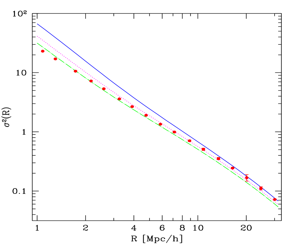
Figure 9: The variance of APM galaxies as a function of smoothing scale $R$ (symbols) compared to the predictions for galaxies as in Eq.(46) with $m_{\rm cut}=10^{11}M_{\sun}$/h (dot-dashed) and galaxies from Eq.(54) (solid) with $a_{1}=1.2$, $a_{2}=0.9$, $m_{\rm cut}=0.8\times 10^{10}M_{\sun}/h$ and $m_{0}=6\times 10^{10}M_{\sun}/h$. Dotted lines show the predictions for using Eq. (54) with the parameter values in Eq. (57).

If we impose no further constraint on the high-mass slope $a_{2}$, we find that the maximum skewness (at $R=20$Mpc/h) is $S_{3}=3$ for the ST mass function (with $a_{2}=1$) and $S_{3}=3.1$ for the PS mass function (with $a_{2}=1.1$). However, such a high value for $a_{2}$ means that 1-halo terms are not suppressed with respect to the mass, and thus the variance and skewness at scales $R\approx 1-5$Mpc/h are much larger than observed. If we restrict $a_{2}\mathrel{\mathchoice{\lower 3.6pt\vbox{\halign{$\mathsurround=0pt\displaystyle\hfill#\hfil$\cr<\crcr\sim\crcr}}}{\lower 3.6pt\vbox{\halign{$\mathsurround=0pt\textstyle\hfill#\hfil$\cr<\crcr\sim\crcr}}}{\lower 3.6pt\vbox{\halign{$\mathsurround=0pt\scriptstyle\hfill#\hfil$\cr<\crcr\sim\crcr}}}{\lower 3.6pt\vbox{\halign{$\mathsurround=0pt\scriptscriptstyle\hfill#\hfil$\cr<\crcr\sim\crcr}}}}0.9$, we find that the maximum skewness for the PS mass function becomes $S_{3}=2.4$, uncomfortably small for APM galaxies (but see below for discussion of APM deprojection issues). For the ST mass function we find that values as high as $S_{3}=2.64$ are possible (with $S_{4}=12.6$), this requires in addition that $a_{1}\approx a_{2}=0.9$ and $m_{\rm cut}\mathrel{\mathchoice{\lower 3.6pt\vbox{\halign{$\mathsurround=0pt\displaystyle\hfill#\hfil$\cr<\crcr\sim\crcr}}}{\lower 3.6pt\vbox{\halign{$\mathsurround=0pt\textstyle\hfill#\hfil$\cr<\crcr\sim\crcr}}}{\lower 3.6pt\vbox{\halign{$\mathsurround=0pt\scriptstyle\hfill#\hfil$\cr<\crcr\sim\crcr}}}{\lower 3.6pt\vbox{\halign{$\mathsurround=0pt\scriptscriptstyle\hfill#\hfil$\cr<\crcr\sim\crcr}}}}10^{10}M_{\sun}/h$, so galaxy formation is relatively efficient in small-mass halos. This values are insensitive to $m_{0}$, as $a_{1}\approx a_{2}$ and the large-scale clustering is insensitive to the distribution of galaxies within halos. Essentially, in this model galaxies trace as much as possible the dark matter. However, as shown in Figs. (9-10) in solid lines ($m_{\rm cut}=8\times 10^{9}M_{\sun}/h$, $m_{0}=6\times 10^{10}M_{\sun}/h$, $a_{1}=1.2$, $a_{2}=0.9$), the small-scale variance and skewness are overestimated in this model. So, further suppression of galaxy formation in high-mass halos is required, $a_{2}<0.9$. Similarly, the galaxy model of Eq.(46) (dot-dashed lines in Figs. (9-10)) suffers from the same problem for the skewness.

Before we turn to constraints derived from small-scale clustering, we should note that these depend on at least two additional assumptions (rather than just the $N_{\rm gal}(m)$ relation). First, we are assuming that galaxies trace the dark matter profile. Fig. 2 in Diaferio et al. (1999) shows that this cannot be true for both red and blue galaxies. The blue semianalytic galaxies, which should be more like the ones in the APM survey, are preferentially located in the outer regions of their parent halos. In the semianalytic models, this happens because, in the time it takes for a galaxy’s orbit to decay (by dynamical friction) from the edge of its parent halo to the centre, its stars age, so its colour changes from blue to red. Blue galaxies on approximately radial orbits which might pass close to the halo centre spend most of their time far from the centre anyway. As a result, most galaxies near the halo centre are red, and those further out are blue. To mimic this effect, we have studied what happens to our model predictions if we decrease the concentration parameter by a factor of two; as explained above, this decreases the variance but it does not change the ratio of moments such as the skewness appreciably, so our results seem robust to this effect.

Second, recall that we are assuming that halo-halo correlations are well described by leading order PT. In the case of the clustering of dark matter, this was well justified because at scales where exclusion effects become important (invalidating the extrapolation from PT), 1-halo terms dominate over halo-halo correlation contributions. For galaxies this may not be true anymore, particularly since many small mass halos host at most one galaxy, so the 1-halo term from these halos is suppressed. For example, we find that at 3 Mpc/h, the contributions of 1-halo and 2-halo terms to the variance and the third moment of the galaxy counts are comparable, whereas this scale is about 5 Mpc/h for the dark matter. If one assumes that exclusion effects suppress the contribution of 2-halo terms (see e.g. Fig. 5 in Mo & White 1996, or the analytic treatment of exclusion effects in Sheth & Lemson 1999), one might conclude that the skewness is higher than what we get by including 2-halo contributions using PT, since these affect more the square of the variance than the third moment. On the other hand, Mo, Jing & White (1997) show that, on scales smaller than the non-linear scale, our formulae for the 3-halo and 4-halo terms significantly overestimate the skewness and kurtosis of the haloes in their simulations (see the bottom right panels of their Figs. 3 and 4). Therefore, although these exclusion effects may conspire to approximately cancel out in the end, we should bear in mind that non-trivial behavior from exclusion effects can invalidate our conclusions from clustering statistics at small scales.

Modulo these caveats, if we impose the additional constraint that at small scales, e.g. $R=1$Mpc/h, $(S_{3})_{\rm gal}\mathrel{\mathchoice{\lower 3.6pt\vbox{\halign{$\mathsurround=0pt\displaystyle\hfill#\hfil$\cr<\crcr\sim\crcr}}}{\lower 3.6pt\vbox{\halign{$\mathsurround=0pt\textstyle\hfill#\hfil$\cr<\crcr\sim\crcr}}}{\lower 3.6pt\vbox{\halign{$\mathsurround=0pt\scriptstyle\hfill#\hfil$\cr<\crcr\sim\crcr}}}{\lower 3.6pt\vbox{\halign{$\mathsurround=0pt\scriptscriptstyle\hfill#\hfil$\cr<\crcr\sim\crcr}}}}6$, we find models with parameters

$$m_{\rm cut} = 4\times 10^{9}M_{\sun}/h,\ \ \ \ \ m_{0}=8\times 10^{11}M_{\sun}/h,\ \ \ \ \ a_{1}=1,\ \ \ \ \ a_{2}=0.8,$$ (57)

$$m_{\rm cut} = 2.5\times 10^{10}M_{\sun}/h,\ \ \ \ \ m_{0}=10^{12}M_{\sun}/h,\ \ \ \ \ a_{1}=0.8,\ \ \ \ \ a_{2}=0.8,$$ (58)

$$m_{\rm cut} = 6\times 10^{10}M_{\sun}/h,\ \ \ \ \ m_{0}=1.2\times 10^{12}M_{\sun}/h,\ \ \ \ \ a_{1}=0.6,\ \ \ \ \ a_{2}=0.8,$$ (59)

the first of which is shown in Figs. 9-10 as dotted lines (the others have very similar behavior). However, all these models predict a small scale variance which is too large; in fact in Fig. 9 we have used a concentration parameter a factor of two smaller than Eq.(12) to decrease the small-scale variance . We were unable to find a model which matched both the variance and skewness of the APM survey at all scales. Therefore, we conclude that the skewness provides a stringent constraint on models of galaxy formation. In particular, the relatively large skewness at large scales and relatively small skewness at small scales provide opposite requirements on the number of galaxies per halo for massive halos. The “large” value of the skewness at large scales requires that galaxies trace mass; however the small value of the skewness at small scales requires that galaxy formation be suppressed in massive halos.

In deprojecting from angular to three-dimensional space, Gaztañaga (1994,1995) assumed the validity of the hierarchical ansatz for the three- and higher-order correlation functions. At large scales, however, PT predicts that the hierarchy of correlation functions is not a simple hierarchical model with constant amplitudes, but rather the amplitudes depend strongly on the shape of the configuration (i.e. the bispectrum depends on the triangle configuration). This can affect the deprojection (Bernardeau 1995; Gaztañaga & Bernardeau 1998); in particular it can lower the three-dimensional skewness and higher-order moments deduced from the angular data, perhaps by as much as 20% at $R\mathrel{\mathchoice{\lower 3.6pt\vbox{\halign{$\mathsurround=0pt\displaystyle\hfill#\hfil$\cr>\crcr\sim\crcr}}}{\lower 3.6pt\vbox{\halign{$\mathsurround=0pt\textstyle\hfill#\hfil$\cr>\crcr\sim\crcr}}}{\lower 3.6pt\vbox{\halign{$\mathsurround=0pt\scriptstyle\hfill#\hfil$\cr>\crcr\sim\crcr}}}{\lower 3.6pt\vbox{\halign{$\mathsurround=0pt\scriptscriptstyle\hfill#\hfil$\cr>\crcr\sim\crcr}}}}10$Mpc/h (Gaztañaga, private communication). At large scales, at least, this would improve the agreement with halo-model predictions.

6 Conclusions

We used the formalism of Scherrer & Bertschinger (1991) to construct an analytic model of the dark matter and of galaxies. For the dark matter, we find that the predictions are in good agreement with numerical simulations, except for the configuration dependence of the bispectrum at small scales. This (numerically small) disagreement can be traced to the assumption that halo profiles are spherically symmetric; in reality the halos generically found in CDM simulations are triaxial. In general, halo models provide accuracy no better than $20\%$ when compared to simulations. However, as N-body results converge on the values of the ingredients of halo models (profiles, mass functions, etc.), their predictions will improve.

We showed how the finite volume of the simulation box can significantly affect the results of higher-order statistics, due to the fact that small boxes have a deficit of massive halos. In particular, we showed that, by making suitable cuts in halo mass function, we were able to reproduce the observed behavior of the bispectrum in small-box (100 Mpc/h) simulations. At small scales, halo models predict a significant departure from the hierarchical scaling, unless the low-mass dependence of the concentration parameter, the mass function, and the small-scale slope of the halo profile are different from the currently accepted values. Unfortunately, the limited resolution of our simulations cannot test these predictions. We caution that Ma & Fry’s (2000) conclusion about the breakdown of the hierarchical ansatz in numerical simulations is premature as their results are likely to suffer from finite volume effects and inadequate resolution.

If galaxies in individual dark matter halos trace the dark matter profiles, galaxy clustering is completely determined within halo models by specifying the moments of galaxy counts as a function of halo mass. In general, suppression of galaxy formation in large-mass halos leads to a power-law like behavior for the galaxy power spectrum and higher-order moments which are smaller than for the dark matter. This is similar to what is observed in galaxy surveys. However, a quantitative comparison with counts-in-cells statistics in the APM survey puts stringent constraints on the galaxy counts as a function of halo mass. At large scales, these require that galaxies trace the mass as closely as possible, implying that galaxy formation is relatively efficient even in small-mass halos. In addition, the small-scale behavior of the skewness requires a high-mass slope for the $N_{\rm gal}(m)$ relation of about $a_{2}=0.8$, although we found no model which simultaneously fits the small scale value of the second moment. The parameters of our “best fit models” are given in Eqs. (57-59). These constraints are independent of those derived from the luminosity function and Tully-Fisher relation which are sensitive to the overall amplitude of the galaxy counts as a function of halo mass.

Clearly, halo models provide a useful framework within which to address many interesting questions about galaxy clustering, and also related topics such as galaxy-galaxy and quasar-galaxy lensing. Our treatment should be of particular interest for the interpretation of clustering in future galaxy surveys, such as SDSS and 2dF. In these cases, however, redshift distortions of clustering must also be taken into account. We plan to address this issue and others relevant to upcoming galaxy surveys in the near future.

- (1) Barnes, J., & Efstathiou, G. 1987, ApJ, 319, 575
- (2) Benson, A.J., Cole, S., Frenk, C.S., Baugh, C.M., & Lacey, C.G. 2000, MNRAS, 311, 793
- (3) Bernardeau F. 1994, ApJ, 433, 1
- (4) Bernardeau F. 1995, A&A, 301, 309
- (5) Bullock, J.S., Kolatt, T.S., Sigad, Y., Somerville, R.S., Kravtsov, A.V., Klypin, A.A., Primack, J.R., Dekel, A. 1999, astro-ph/9908159
- (6) Catelan, P., Lucchin, F., Matarrese, S., & Porciani, C. 1998, MNRAS, 297, 692
- (7) Colombi, S., Bouchet, F. R., & Hernquist, L. 1996, ApJ, 465, 14
- (8) Cooray, A., & Hu, W. 2000, astro-ph/0004151
- (9) Couchman H. M. P., Thomas P. A., Pearce F. R. 1995, ApJ, 452, 797
- (10) Diaferio, A., Kauffmann, G., Colberg, J.M., & White, S.D.M. 1999, MNRAS, 307, 537
- (11) Durrer, R., Juszkiewicz, R., Kunz, M., & Uzan, J-P. 2000, astro-ph/0005087
- (12) Frenk, C.S., White, S.D.M., Davis, M., & Efstathiou, G. 1988, ApJ, 327, 507
- (13) Frieman, J., & Gaztañaga, E. 1994, ApJ, 425, 392
- (14) Frieman, J., & Gaztañaga, E. 1999, ApJ, 521, L83
- (15) Fry, J. N. 1984, ApJ, 279, 499
- (16) Fry J. N., Gaztañaga E. 1993, ApJ, 413, 447
- (17) Fry, J. N. 1994, Phys. Rev. Lett., 73, 215
- (18) Fry J. N., Scherrer, R. 1994, ApJ, 429, 36
- (19) Gaztañaga, E. 1994, MNRAS, 268, 913
- (20) Gaztañaga, E. 1995, ApJ, 454, 561
- (21) Gaztañaga, E., Mähönen, P. 1996, ApJ, 462, L1
- (22) Gaztañaga, E., Bernardeau F. 1998, A&A, 331, 829
- (23) Gaztañaga, E., Fosalba, P. 1998, MNRAS, 301, 524
- (24) Hamilton, A. J. S., Kumar, P., Lu, E., & Matthews, A. 1991, ApJ, 374, L1
- (25) Hui, L., & Gaztañaga, E., 1999, ApJ, 519, 622
- (26) Jain, B. 1997, MNRAS, 287, 687
- (27) Jain, B., Mo, H.J. & White, S. D. M. 1995, MNRAS, 276, L25
- (28) Jenkins, A., Frenk, C.S., White, S.D.M., Colberg, J.C., Cole, S., Evrard, A.E., Yoshida, N. 2000, astro-ph/0005260
- (29) Jing, Y. P., Mo, H. J., & Börner, G. 1998, ApJ , 494, 1
- (30) Kauffmann, G., Colberg, J.M., Diaferio, A., & White, S.D.M. 1999, MNRAS, 303, 188
- (31) Ma, C-P, & Fry, J.N. 2000, astro-ph/0003343
- (32) Ma, C-P, & Fry, J.N. 2000b, astro-ph/0005233
- (33) Maddox, S.J., Efstathiou, G., Sutherland, W.J., & Loveday, L. 1990, MNRAS, 242, 43
- (34) McClelland, J., & Silk, J. 1977, ApJ, 216, 665
- (35) McClelland, J., & Silk, J. 1977b, ApJ, 217, 331
- (36) McClelland, J., & Silk, J. 1978, ApJS, 36, 389
- (37) Matarrese, S., Verde, L., & Heavens, A.F. 1997, MNRAS, 290, 651
- (38) Mo, H. J., & White, S. D. M. 1996, MNRAS, 282, 347
- (39) Mo, H. J., Jing, Y. P., & White, S. D. M. 1997, MNRAS, 284, 189
- (40) Moore, B., Quinn, T., Governato, F., Stadel, J., & Lake, G. 1999, MNRAS, 310, 1147
- (41) Navarro, J. F., Frenk, C. S., & White, S. D. M. 1996, ApJ, 462, 563
- (42) Navarro, J. F., Frenk, C. S., & White, S. D. M. 1997, ApJ, 490, 493
- (43) Neyman, J., & Scott, E.L. 1952, ApJ, 116, 144
- (44) Peacock, J. A. & Dodds, S. J. 1996, MNRAS, 280, L19
- (45) Peacock, J. A. & Smith, R.E. 2000, astro-ph/0005010
- (46) Peebles, P.J.E. 1974, A&A, 32, 197
- (47) Peebles, P.J.E., 1980, The Large Scale Structure of the Universe. Princeton University Press, Princeton
- (48) Press, W.H., & Schechter, P. 1974, ApJ, 187, 425
- (49) Scherrer, R. J., & Bertschinger, E. 1991, ApJ, 381, 349
- (50) Scoccimarro, R., Colombi, S., Fry, J.N., Frieman, J.A., Hivon, E., & Melott, 1998, ApJ, 496, 586
- (51) Scoccimarro, R., & Frieman, J.A. 1999, ApJ, 520, 35
- (52) Scoccimarro, R. 2000, astro-ph/0004086
- (53) Scoccimarro, R., Feldman, H.A., Fry, J.N., & Frieman, J.A. 2000, astro-ph/0004087
- (54) Seljak, U. 2000, astro-ph/0001493
- (55) Sheth, R. K., & Jain, B. 1997, MNRAS, 285, 231
- (56) Sheth, R. K. 1996, MNRAS, 281, 1124
- (57) Sheth, R. K., & Lemson, G. 1999, MNRAS, 304, 767
- (58) Sheth, R. K., & Tormen, B. 1999, MNRAS, 308, 119
- (59) Sheth, R. K., & Diaferio, A. 2000, in preparation
- (60) Somerville R. S., Primack J. R., 1999, MNRAS, 310,1087
- (61) Szapudi I., Colombi S. 1996, ApJ, 470, 131
- (62) Szapudi I., Colombi S., Jenkins A., Colberg J., 1999, submitted to MNRAS, astro-ph/9912238.
- (63) White, S. D. M., & Frenk, C. S., 1991, ApJ, 379, 52
- (64) White, S. D. M., & Rees, M. J., 1978, MNRAS, 183, 341
- (65) Zurek, W.H., Quinn, P.J., & Salmon, J.K. 1988, ApJ, 330, 519