Kelvin-Helmholtz instability in three dimensional radiative jets

Abstract

The analysis of the stability properties of astrophysical jets against Kelvin-Helmholtz (or shear-layer) instabilities plays a basic role in the understanding the origin and physical characteristics of these objects. Numerical simulations by Bodo et al. (1998) have shown that the three-dimensional non-linear evolution of KH instabilities in supersonic jets is substantially faster than in the two-dimensional case, leading to a cascade of modes towards smaller scales and a very effective mixing and momentum transfer to the ambient medium. On the other hand, Rossi et al. (1997) and Micono et al. (1998) found, in two dimensions, that radiative losses tend to reduce and delay mixing effects and momentum transfer to the ambient medium. In this paper, as a logical next step, we investigate the effects of radiative losses on the stability of 3D supersonic jets, assuming that the internal jet density is initially lower, equal and higher than the ambient medium, respectively. We find that light and equal-density radiative jets evolve in a qualitatively similar fashion with respect to the corresponding adiabatic ones. Conversely, we note substantial differences in the evolution of heavy jets: they remain more collimated and do not spread out, while the momentum gained by the ambient medium stays within $\sim 5$ jet radii.

1 Introduction

Jets that originate from young T Tauri stars in giant molecular clouds and from Active Galactic Nuclei propagate, in a collimated fashion, up to distances $\sim 100-1000$ times their average radii. The question of their endurance against Kelvin-Helmholtz instabilities is a crucial one for understanding the phenomenology of these objects. This issue has been addressed by many authors first in the linear limit (see Birkinshaw 1991 for a review) and, in recent years, through the use of 2D and 3D numerical simulations (see Ferrari 1998 for a review). In particular, recently, Bodo et al. (1998) have examined the differences between two-dimensional and three-dimensional jet evolution, showing that three-dimensional jets undergo faster evolution, enhanced mixing and larger jet momentum depletion. The temporal duration of the shock-dominated phase of the Kelvin-Helmholtz instability evolution is strongly reduced, shocks that form are weaker, and the direct association between structures observed in astrophysical jets and shocks originating as a consequence of the nonlinear development of the Kelvin-Helmholtz instability is more problematic. Moreover, the rapid disruption that three-dimensional jets undergo raises the question as to how jets can survive for the long scale lengths shown by observations. Although relativistic bulk velocities may be a stabilizing factor in extragalactic jets, the stability problem remains crucial for the nonrelativistic jets associated with Young Stellar Objects (YSOs), and radiation might be an important ingredient in this respect.

The interest in radiation effects on the development of Kelvin-Helmholtz instabilities in supersonic jets was motivated by the observation of line-emitting knots in YSO jets. Linear analyses of the stability of radiative jets by Massaglia et al. (1992) and Hardee & Stone (1997), showed that radiation losses typically reduce the growth rates of perturbations. Extending the analysis to nonlinear amplitudes, Rossi et al. (1997) and Micono et al. (1998) found that radiative cooling has noticeable effects on the spatial and temporal evolution of two-dimensional jets; in particular, the action of cooling leads to a longer duration of the initial linear stage and of the shock-dominated stage of the instability; shocks that form appear weaker and the post-shock temperatures smaller; the importance of the mixing phase is reduced and in some case, depending on the jet density, it is totally absent. Studying this problem, Downes & Ray (1998) found a somewhat contrary result with respect to Rossi et al. (1997): from their temporal simulations they concluded that cooling enhances the momentum transfer to the ambient medium, increasing the level of mixing. They suggested that the differences in the two studies might be due to the different geometries adopted: Cartesian in their case, and cylindrical in Rossi et al. (1997).

The goal of the present work is to study the effect of radiative losses on the evolution of the Kelvin-Helmholtz instability in a three-dimensional jet, with particular focus on the issues of mixing and momentum transfer in a system which is not subject to any superimposed symmetry. Moreover, with explicit reference to jets from YSOs, we aim to verify whether the action of cooling is strong enough to prevent a fast disruption of three-dimensional jets, which must survive for the length and time scales that are observed. Specifically, we investigate the behavior of dense, light and equidense jets, and analyze the effects of increasing the amount of energy lost through radiation by changing the value of a radiative control parameter which is directly related to the ratio between the cooling and dynamical time scales.

The plan of the paper is the following: in Section 2 we examine the physical problem and the equations used; the numerical scheme is described in Section 3; Section 4 summarizes the results of our previous studies on the stability of adiabatic jets; the results of our simulations are discussed in Section 5. Finally, a summary and the conclusions are given in Section 6.

2 The physical problem

We study the evolution of a 3D fluid jet, subject to radiative losses; the equations regulating our system are thus the ideal fluid equations for mass, momentum and energy conservation:

$${{\partial\rho}\over{\partial t}}+\nabla\cdot(\rho{\bf{v}})=0\,,\\$$ (1)

$$\rho{{\partial{\bf v}}\over{\partial t}}+\rho({\bf v}\cdot\nabla){\bf v}=-\nabla p\,,\\$$ (2)

$${{\partial p}\over{\partial t}}+({\bf{v}}\cdot\nabla)p-\gamma\ {p\over\rho}\ \left[{{\partial\rho}\over{\partial t}}+({\bf{v}}\cdot\nabla)\rho\right]=(\gamma-1)\ \left({\it\cal Q}-{\it\cal L}\right)$$ (3)

where $p$, $\rho$, and ${\bf v}$ are pressure, density and velocity, $\gamma$ is the ratio of the specific heats, and ${\it\cal L}$ and ${\it\cal Q}$ are respectively the energy loss term and the heating term (assumed here constant, and equal to ${\it\cal L}$ taken at $t=0$); the right hand side of Eq. 3 vanishes in a purely adiabatic case.

We also follow the evolution of the number fraction of the neutral hydrogen atoms $f_{\rm n}$:

$${{\partial f_{\rm n}}\over{\partial t}}+({\bf v}\cdot\nabla)f_{\rm n}=n_{e}[-(c_{\rm i}+c_{\rm r})f_{\rm n}+c_{\rm r}]\,,$$ (4)

where $n_{\rm e}$ is the electron density, and $c_{\rm i}$ and $c_{\rm r}$ are the ionization and recombination coefficients, which depend on the temperature $T$ and on the electron density $n_{\rm e}$ in the following way:

$$c_{\rm i}=1.08\cdot 10^{-8}\cdot 13.6^{-2}\cdot\sqrt{T}\ {\rm e}^{(-157890./T)}\ \ \ \ \ {\rm cm}^{3}\ {\rm s}^{-1}$$ (5)

$$c_{\rm r}=2.6\cdot 10^{-11}/\sqrt{T}\ \ \ \ \ {\rm cm}^{3}\ {\rm s}^{-1}\$$ (6)

(Rossi et al. 1997).

Finally, we trace the jet material by means of a scalar field $\cal T$ whose evolution is followed by integrating the scalar advection equation:

$${{\partial\cal T}\over{\partial t}}+({\bf v}\cdot\nabla){\cal T}=0\ .$$ (7)

Cooling is treated here as in our two previous papers on 2D cooling jets, and the reader is referred to Rossi et al. (1997) for a detailed description. The assumed losses are a reasonable approximation for temperatures $T\mathbin{\raise 2.0pt\hbox{$<$}\hskip-9.0pt\lower 4.0pt\hbox{$\sim$}}$ 35,000 K and shock velocities up to about 80 km s^-1; both conditions are generally fulfilled in YSO jets. We recall, in particular, that we assume here that our jet is composed of atomic gas with solar abundances, and we neglect the formation of molecules and molecular emission. This assumption is consistent with our choice for the initial jet temperature, which is well above the dissociation temperature for the hydrogen molecule.

3 The numerical setup

3.1 The integration method

The hydrodynamical equations are integrated numerically using a three-dimensional version of the Piecewise Parabolic Method code (Colella & Woodward 1984). The code was parallelized through the MPI package. Multidimensionality, as well as the inclusion of radiative losses, are achieved through operator splitting: the PPM code solves the Eqs. 1 - 4) and 7) in a conservative form; where non-conservative terms are present, the physical quantities are updated at the end of the main time step. In addition, the integration time step is constrained by the Courant condition, and is further corrected so that the temperature does not vary by more than 10% in a single step.

3.2 Integration domain, initial and boundary conditions

Our 3D domain $\{(0,D)\times(-R,R)\times(-R,R)\}$, with $D=10\pi a$ and $R=6.7a$ where $a$ is the jet radius, is covered by a $256\times 256\times 256$ grid, and is described by a Cartesian coordinate system $(x,y,z)$.

The initial flow structure is a cylindrical jet, with its symmetry axis lying along the $x$-direction and defined by $(y=0,\ z=0)$. The initial jet velocity is along the $x$-direction. The interface between the jet and the surrounding material is not a vortex-sheet-like interface, but a smoothly varying velocity shear layer. The form of the initial jet velocity profile is thus:

$$V_{x}(y,z)=V_{0}\ {\rm sech}\left[\left({\sqrt{y^{2}+z^{2}}}\over a\right)^{m}\right]\,,$$ (8)

where $V_{0}$ is the velocity on the jet axis, and $m$ is a parameter controlling the interface layer width; in these calculations we set $m=8$ which implies a shear layer thickness of approximately 0.4 jet radii.

The initial structure of the density in our domain is defined by:

$${{\rho_{0}(y,z)}\over\rho_{0,jet}}=\nu-(\nu-1)\ {\rm sech}\left[\left({\sqrt{y^{2}+z^{2}}}\over a\right)^{m}\right]\,,$$ (9)

where $\nu$ is the ratio of the density at $r=\sqrt{y^{2}+z^{2}}=\infty$, to that on the jet axis $(y=z=0)$ at the initial time.

We assume that the jet is initially in ionization equilibrium, and in pressure equilibrium with its surroundings (with an initially uniform imposed pressure distribution).

Finally, we impose the following initial conditions for the passive tracer $\cal T$:

$$\cal T=\left\{\begin{array}[]{cc}\;1,&\quad r<1\\ \;0,&\quad r>1\,.\end{array}\right.$$ (10)

so that we are able to follow the jet material during its subsequent evolution.

This initial configuration is then perturbed at $t=0$; we perturb the transverse velocities $V_{y}$ and $V_{z}$, so that a wide range of modes can be excited. In order to mainly excite the helical mode, we choose the following functional form for the transverse velocities:

$$V_{y}(x,y,z)=V_{y,0}\ {\rm sech}\left[\left({\sqrt{y^{2}+z^{2}}}\over a\right)^{m}\right]\times{}$$ (11)

$${}\qquad\qquad\,\times{1\over n}\ \sum_{j=1}^{n}\sin(jk_{0}x+\phi_{j})\,,$$

$$V_{z}(x,y,z)=V_{z,0}\ {\rm sech}\left[\left({\sqrt{y^{2}+z^{2}}}\over a\right)^{m}\right]\times{}$$ (12)

$${}\qquad\qquad\,\times{1\over n}\ \sum_{j=1}^{n}\cos(jk_{0}x+\phi_{j})\,,$$

where $V_{y,0}=V_{z,0}=0.05V_{0}$ is the amplitude of the initial perturbation, $\{\phi_{j}\}$ are the phase shifts of the various Fourier components, $n=8$ and $k_{0}=2\pi/D$.

As regards the behavior at the boundaries, we adopt free outflow boundary conditions at the upper and lower boundaries in the $y$ and $z$ directions, by setting the gradient of every variable to zero. The central region of the domain, $-3a<y<3a$, $-3a<z<3a$, is covered uniformly by 150 grid points in the radial direction (with the jet itself initially occupying 50 grid points at $t=0$); at larger distances from the jet axis, both the $y$ and the $z$ mesh sizes increase accordingly to the scaling laws $\Delta y_{j+1}=1.02\Delta y_{j}$ and $\Delta z_{k+1}=1.02\Delta z_{k}$ respectively. The grid along the $x$ direction is instead uniform, and the boundary conditions are periodic. This choice implies a temporal approach to the study of the instability evolution, as opposed to a spatial approach where inflow and outflow conditions are applied at the left and right boundary respectively, along the jet flow direction. We refer to Rossi et al. (1997) and Bodo et al. (1998) for a more detailed discussion of boundary conditions, grid settings and comparison between the temporal and spatial approaches.

3.3 Scaling and parameters

Our calculations are carried out in non-dimensional form. Distances are thus measured in units of the jet radius $a$, velocities are scaled to the isothermal sound speed $c_{\rm s}$, evaluated on the jet axis and at the initial time $t=0$. Accordingly, time is then measured in units of the sound crossing time $t_{\rm cr}$.

The dynamical control parameters for our problem are the Mach number M($=V_{0}/(c_{\rm s}\sqrt{\gamma})$) and the density ratio $\nu=\rho_{\infty}/\rho_{\rm jet}$. The treatment of cooling introduces two more parameters in our calculations, namely the initial temperature on the jet axis $T_{0}$ and the ratio $\tau_{\rm rad}$ between radiative cooling time $t_{\rm rad}=p/[(\gamma-1){\cal L}]$ and the sound crossing time. Fixing $\tau_{\rm rad}$ is analogous to fixing the product of the jet particle density and the jet radius $n_{0}a$, which was selected in our calculations since it has more direct observational meaning (Rossi et al. 1997).

In our simulations, we fixed the Mach number $M=10$ and we selected three values for the ratio $\nu$ between the external and the jet material, i.e. $\nu=0.1$ (overdense jet), $\nu=1$ (isodense jet) and $\nu=10$ (underdense jet). The initial temperature on the jet axis was always $T_{0}=10,000$ K, and for the product of the jet particle density and the jet radius we selected the value $n_{0}a=5\times 10^{17}\ {\rm cm}^{-2}$, which is consistent, for example, with a jet radius $a=5\times 10^{15}\ {\rm cm}$ and a jet particle density $n_{0}=100{\rm cm}^{-3}$; however, we recall that our results are valid for all pairs of values of $n_{0}$ and $a$ for which their product is constant.

For the equidense jet ($\nu=1$) case we performed a simulation with the value $n_{0}a=5\times 10^{18}\ {\rm cm}^{-2}$ in order to study the effect of varying the radiative cooling time on the instability evolution.

In Table 1 we summarize the simulations discussed in the present paper, with the values of the relevant parameters.

Table 1:

Simulation	$M$	$\nu$	$T_{0}$	$n_{0}a$
A	10	0.1	$10^{4}$ K	$5.\times 10^{17}\ {\rm cm}^{-2}$
B	10	10.	$10^{4}$ K	$5.\times 10^{17}\ {\rm cm}^{-2}$
C	10	1.	$10^{4}$ K	$5.\times 10^{17}\ {\rm cm}^{-2}$
D	10	1.	$10^{4}$ K	$5.\times 10^{18}\ {\rm cm}^{-2}$

4 Results of previous studies

4.1 Stages of the instability evolution

Previous studies of the temporal (Bodo et al. 1994, 1995, Rossi et al. 1997) and spatial (Micono et al. 1998) evolution of the Kelvin-Helmholtz instability in two-dimensional jets allowed us to distinguish four stages of evolution; they were identified in adiabatic and cooling jets in the spatial and temporal approach, in slab and cylindrical geometry; their features, as for example the onset time, the duration, the morphological and physical evolution of the jet during each stage, were dependent on the parameters adopted, although the general trend was common to all studied cases. We recall in the following the main features of each evolutionary stage:

• Stage 1: the unstable modes excited by the perturbation grow in accord with the linear theory. In the latter portion of this stage, the growth of the modes leads to the formation of internal shocks.

• Stage 2 : the growth of internal shocks is accompanied by a global deformation of the jet, which thus drives shocks in the external medium. These shocks can carry momentum and energy away from the jet, and transfer them to the external medium.

• Stage 3 : as a consequence of the shock evolution, mixing between jet and external material begins to occur. The longitudinal momentum, which is initially concentrated inside the jet radius, is spread over a much larger region by the spreading of the jet material.

• Stage 4: in this final state, the jet attains a statistically quasi-stationary state.

The effects of radiative losses on the instability have been traced by Rossi et al. (1997) and Micono et al. (1998). The main differences of this analysis with respect to the adiabatic case are: i) a longer duration of stages 1 and 2 of the evolution; ii) a decrease of the shock strength and of the post-shock temperatures, and iii) a general reduction of the importance of the mixing phase (depending on the values of $\nu$ and $n_{0}a$), with a complete absence of the mixing phase for high values of $n_{0}a$.

4.2 2D vs 3D behaviour

In this section we summarize the main results obtained by Bodo et al. (1998) in their comparative analysis of 2D and 3D adiabatic jets. Bodo et al. (1998) adopted a Cartesian geometry and a temporal approach (i.e., periodic boundary conditions in the direction of the jet axis), and superimposed helical perturbations onto the initial transverse velocities (see also below).

The expected differences are mainly due to two factors: first, there are many more unstable modes in three dimensions than in two dimensions, and the growth rates of the 3D modes can predominate. Second, it is well-known that turbulence in two and three dimensions differs substantially, especially as far as the mixing properties are concerned. Both effects – the presence of unstable high-wavenumber modes, and the cascade to high wave numbers via nonlinear interactions – can lead to the formation of small-scale structures that are not observed in two dimensions.

The main features observed by Bodo et al. (1998) in the evolution of over-dense and under-dense three-dimensional adiabatic jets, compared to analogous two-dimensional slab jets, can be summarized as follows:

• Faster evolution.

• Absence of a clear separation of stages 2 and 3 of the instability (as defined in section 4.1).

• More rapid development of small-scale structures due to the growth of linearly unstable higher order (azimuthal number $\leq 2$) fluting modes and, at advanced times, to a cascade to small scales through nonlinear turbulent processes.

• Enhanced material mixing between the jet and the ambient medium; more effective and faster momentum transfer from jet to the ambient medium.

• Enhanced jet broadening.

• Similar evolution of the largest-scale structures.

• Similar asymptotic states (although reached at very different times).

5 Results

5.1 Heavy jets ($\nu=0.1$)

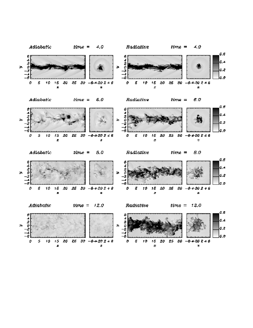
Figure 1: Grey-scale images of the density distribution for heavy ($\nu=0.1$) adiabatic (left column) and radiative (right column) jets; 2D cuts at a fixed $z$ ($z=0$) and at a fixed $x$ ($x=5\pi$).

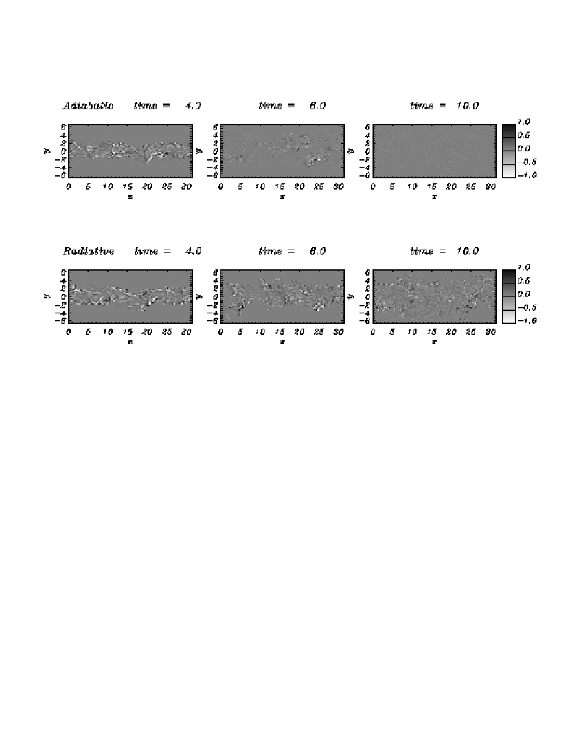
Figure 2: Grey-scale images of two dimensional cuts of the density Laplacian, in the plane $z=0$

In this section we present the results of the calculations for an adiabatic jet and a cooling jet with Mach number $M=10$ and density ratio $\nu=0.1$. We carried out the simulation for $t=12$ units of sound crossing time, since at this time the adiabatic jet reaches the boundaries in the $y$ and $z$ directions.

In Fig. 1 we show grey-scale images of two-dimensional cuts of the jet density, in the $z=0$ plane (i.e., a longitudinal cut in the $(xy)$ plane in the middle of the domain) and in the $x=5\pi$ plane (i.e. a transverse cut in the $(yz)$ plane in the middle of the domain), for the radiative and adiabatic jets at different stages of the evolution.

At time $t=4$ the situations is similar for the adiabatic and cooling jets: the instability has already entered the acoustic phase, with the development of shock waves driven by the jet into the external medium, in correspondence to the major “kinks” caused by the growth of the fundamental helical mode excited by the imposed perturbation. Acoustic waves are driven in the external medium, as it can be clearly seen in the upper panels of Fig. 1. Already at this early stage, a little amount of external material is being entrained by the jet, as a result of the growth of higher order fluting modes that produce short scale ripples on the surface of the jet.

At time $t=6$ the radiative jet is still shock-dominated, although the disturbances induced on the jet surface have grown in amplitude and the amount of entrained ambient medium has increased. In contrast, the adiabatic jet appears to have fully entered the mixing phase; no trace of the coherent large-scale deformations induced by the fundamental helical Kelvin-Helmholtz mode can be discerned. As the evolution proceeds, the adiabatic jet appears to be completely mixed with the ambient medium ($t=8$, Fig. 1), while the jet subject to radiative losses maintains its collimation up to the latest time in our calculations, $t=12$; at this time both jets have reached stage 4 of the instability evolution, i.e., a statistically “quasi-stationary” stage. The comparison between the adiabatic and radiative jets in Fig. 1 also conveys the impression that the adiabatic jet has become much wider than its radiative counterpart. To analyze this effect in more detail, we have computed the radial distribution of velocity averaged over the longitudinal and azimuthal directions and we have defined the jet radius as the radius at which this averaged velocity drops to one half of its maximum value (found at $r=0$). Fig. 3c) shows the evolution of this radius as a function of time; we see from the figure that in fact the adiabatic jet widens much more than the radiative one.

In Fig. 2 we show a two-dimensional cut of the Laplacian of the density in the plane $z=0$ (the Laplacian of the density is a valuable tool to mark the presence of shock waves in the flow, and is widely used in gas dynamics).  Upon examining this figure, we can follow the same evolutionary path described above. The Laplacians at time $t=2$ are not shown since no significant feature can be detected: both jets are in fact still in the linear phase (stage 1) of the evolution. When the perturbations steepen into shock waves, the jet enters the acoustic phase ($t=4$). The duration of the acoustic phase is longer for the radiative jet, where strong shock waves survive up to $t=10$; for the adiabatic jet, instead, shock waves are damped by the vigorous mixing that occurs already during the acoustic stage: after time $t=6$, no shocks can be detected in the flow, and turbulent mixing dominates.

Figure 3: Panel (a) shows a plot of the tracer entropy for the radiative (solid line) and adiabatic (dashed line) jets as a function of time (for the analytical and physical definition of tracer entropy see Bodo et al. 1995); panel (b) shows a plot of the jet momentum for the radiative (solid line) and adiabatic (dashed line) jets as a function of time. Panel (c) provides a plot of the temporal evolution of the jet radius for the radiative (solid line) and adiabatic (dashed line) cases . All the plots are for the heavy jet case ($\nu=0.1$).

Figure 4: Panel (a): ambient medium momentum as a function of the distance from the jet axis. Panel (b): ambient medium momentum versus the corresponding value of the density. In both panels we plot the trends referring to heavy radiative (solid line), and adiabatic (dashed line) jets at different times.

In panel (a) of Fig. 3 we plot the tracer entropy $\cal W$ vs. time, for the adiabatic (dashed line) and radiative (solid line) dense jets. $\cal W$ measures the departure of the tracer’s distribution from the initial form (${\cal T}=1$ for the jet material and ${\cal T}=0$ for the external material; see Bodo et al. (1995) for the mathematical definition of $\cal W$). Up to time $t=2$ the jet is still in the linear phase of the evolution, and the entropy is almost constant, since the tracer distribution does not differ substantially from the initial one. As time elapses, the jet goes through stages 2 and 3 of the evolution, during which the entropy grows, reaching a quasi-constant value at the end of the evolution.

In Fig. 3b) we plot the momentum of the radiative (solid line) and adiabatic (dashed line) jets, normalized to the initial values, as a function of time. In both cases, the jets start losing momentum early in time; the final momentum loss is dramatic, since at time $t=12$ radiative and adiabatic jets have lost almost 80% of their initial momentum. Fig. 3b) shows that the amount of momentum lost by the radiative and the adiabatic jets is similar; the momentum loss is slightly greater for the radiative jet. This result seems to be in contradiction with the behavior described previously: if we assume that the quantity of momentum lost is a valid indicator of the instability effects, then we would expect that the radiative jet is equally or more unstable than the adiabatic jet; on the other hand, we saw that radiative cooling acts to reduce the development of mixing and to conserve the collimation of the jet for longer times. In fact, as we have seen above, the jet widening in the adiabatic case is larger than in the radiative case; one could then expect that the amount of entrained material would be much larger in the adiabatic case, and correspondingly the residual jet momentum much lower. This apparent discrepancy can be explained if we analyze how momentum is lost by the jet in the two cases.

The rate of momentum transfer is almost similar for the cooling and adiabatic jets, but the radiative jet accelerates only the ambient medium located very near the jet itself; in contrast, the adiabatic jet expands and entrains material over a much larger radial extent, accelerating it until at the end of our calculations all the ambient medium in our computational domain has a non-zero velocity in the longitudinal direction; this trend appears clearly in Fig. 4a), where the amount of momentum acquired by the external medium at different times is shown as a function of the distance from the initial jet axis.

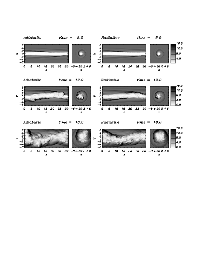
Figure 5: Grey-scale images of the density distribution for light ($\nu=10$) adiabatic (left column) and radiative (right column) jets; 2D cuts at a fixed $z$ ($z=0$) and at a fixed $x$ ($x=5\pi$).

The typical velocities attained by the accelerated ambient medium in the two cases are similar (for example, the maximum velocity of the material with ${\cal T}<0.1$ at t=10 is $\sim 6.8$ for both cases), but the adiabatic jet accelerates a larger radial volume of ambient material. A similar amount of transferred momentum is thus achieved in the two cases only if in the radiative case denser ambient material is accelerated. That this is the case is demonstrated by Fig. 4b), which shows the distribution of momentum in the external medium versus the corresponding value of the density for the radiative and adiabatic jets: we characterized each volume of ambient medium by its values of momentum and density, divided the density range into density bins, and integrated the momentum over each density bin, obtaining the distribution showed in Fig. 4b. This figure shows that the typical densities of the entrained material are much larger in the radiative case than in the adiabatic case; furthermore, the total mass of the entrained material turns out to be of the same order in both cases. We can understand this if we note that the initial shocks driven by the adiabatic jets heat the external gas, which consequently expands and thus lowers its density. In the radiative case, cooling suppresses the expansion, leading in contrast to a compression of the shocked material; the momentum acquired by the external medium resides largely in material whose density is up to ten times higher than the initial external density. In addition we must remember that this shock-induced compression can be very effective in the radiative case since strong shock waves survive for long times, from $t=4$ to $t=10$ (see Fig. 2).

5.2 Light jets ($\nu=10$)

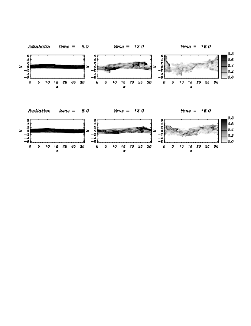
Figure 6: Grey-scale images of the jet density (i.e., of the product between density and tracer) distribution for light ($\nu=10$) adiabatic (upper line) and radiative (lower line) jets; 2D cuts at $z=0$.

A quick glimpse at Fig. 5, which displays two-dimensional grey-scale cuts of the density at different times in the $z=0$ and $x=5\pi$ planes, shows that radiative losses in underdense jets have little effect on the instability evolution, which is slower with respect to the previously examined cases: the linear phase of the instability (stage 1) lasts until time $t=8$ when the first shocks appear in both the adiabatic and in the cooling jets. The density distributions shown in Fig. 5 cannot show details inside the jet because the grey-scale saturates there. Therefore, in order to obtain better views of the jet structures, we show in Fig. 6 grey-scale two-dimensional cuts of the product of the tracer and the density at different times. From these figures we can see that shocks form inside the jet and in the external medium, corresponding to the kinks induced by the fundamental helical mode, and persist for long times: at time $t=16$, when mixing has taken place and the jet diameter has considerably widened, a few weak shocks can still be detected both in the adiabatic and cooling jets.

The growth of the higher order fluting modes is delayed in time, and mixing occurs later, mainly because of the inertia of the external medium. The onset of mixing occurs between times $t=10$ and $t=12$, and is initially limited to the more external layers of the jet. At later times (e.g., time $t=18$ in Fig. 5) the action of mixing is not disruptive, and the jet maintains its collimation.

Figure 7: In panel (a) we show a plot of the tracer entropy for the radiative (solid line) and adiabatic (dashed line) jets as a function of time; in panel (b) we show a plot of the jet momentum for the radiative (solid line) and adiabatic (dashed line) jets as a function of time. In panel (c) the temporal evolution of the jet radius for the radiative (solid line) and adiabatic (dashed line) cases is plotted. All the plots are for the light jet case ($\nu=10$).

The transition between the evolutionary stages is well depicted by the tracer entropy, plotted in Fig. 7a): entropy remains almost constant, increasing slowly for the first 8-10 sound crossing times, when the perturbations grow linearly and the first shocks form. A larger increase of the entropy occurs at later times, with a steeper growth for the adiabatic case (which reaches the quasi-stationary phase earlier, at $t\sim 15$ as compared to $t\sim 18$ for the radiative case). The jet momentum is plotted in Fig. 7b) as a function of time; we can see that the momentum behavior is similar to the entropy behavior: the drop in the jet momentum appears to be steeper for the adiabatic case, but it stops earlier so that the total amount of momentum lost by the jet material is about the same for the two cases ($\sim$ 90% of the initial value). A more careful comparison between the behaviors of entropy and momentum shows that the phase of steeper decrease of momentum begins earlier than the phase of steeper increase of entropy. In this case we then have a distinct phase 2 (acoustic phase) of the evolution in which momentum is mainly lost through shocks.

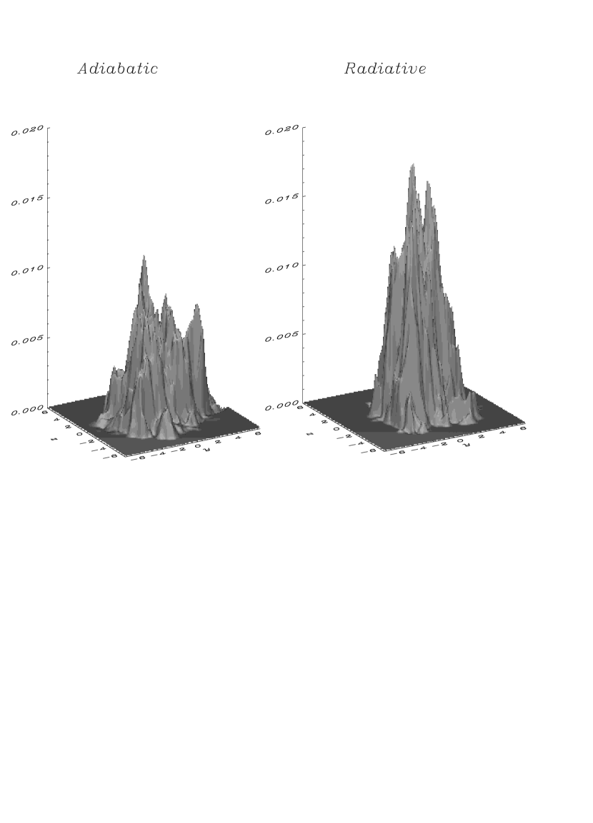
Figure 8: Longitudinally averaged distribution of the jet momentum at time t=18 for the adiabatic and radiative light jets.

The largest differences between the adiabatic and the radiative cases can be seen in the last stage of the evolution: looking at Figs. 5 and 6 at times $t=16$ and $t=18$, we see that the adiabatic jet appears to be wider than the radiative one. This is confirmed by Fig. 7c), which shows the behavior of the jet radius, as defined in the previous subsection, as a function of time. The difference between the adiabatic and the radiative cases however is not so large as for the dense jets. This same effect can also be seen in the jet momentum distribution: in Fig. 8 we show the grey-scale distribution in the (yz) plane of the average of the jet momentum over the longitudinal direction for the two cases; we see that the distribution is wider for the adiabatic jet. Since the total amount of momentum retained by the jet is about the same in the two cases, we also find that the maximum value of the jet momentum, located at a position corresponding to the initial jet axis, is smaller for the adiabatic jet (about half the maximum value of the cooling jet momentum).

From the above description we can conclude that – in contrast to the heavy jet case – the presence of radiative losses does not strongly modify the overall evolution of the instability in a light jet. To investigate the reasons for this behaviour, we plotted in Fig. 9 the total radiative power (jet plus ambient medium) for heavy, light and equal-density jets. In each case, the peak in the emission takes place shortly after the onset of the acoustic stage, when shocks are well developed and not yet disrupted by mixing.

Figure 9: Power lost through radiation by heavy (solid line), light (dotted line) and equal-density jets (dashed line). Units are normalized to the peak emission in the $\nu=0.1$ jet.

The amount of energy lost through radiation is at least an order of magnitude smaller in the light jet compared to the dense jet. The reasons for this behavior are many; first, the growth of the helical mode in the dense jet drives larger amplitude kinks when compared to those observed in the light jet; in this way the shock fronts are wider in the $\nu=0.1$ jet, and a larger amount of material is compressed, heated and ultimately cooled through radiation. In addition, the wavelength of the most unstable mode may play an important role: a shorter wavelength, typical of dense jets (see Hardee & Norman 1988) leads to the formation of a higher number of shocks in a short time, increasing the efficiency of the cooling mechanism at shocks (compare also Figs. 1 and 5). We also note that the ambient medium gives a significant contribution to the subtraction of energy from the system, in particular when dense and equal-density jets are concerned; in fact, shocks are driven by the jet into the ambient medium, and they propagate in the external regions immediately surrounding the jets; the spatial extension of these shocks can be consistently larger that in the jet’s body.

5.3 Equal-density jets ($\nu=1$)

When studying equal-density radiative jets with the same value of $n_{0}a$ as considered in the previous cases ($n_{0}a=5\times 10^{17}$ cm^-2, consistent, for example, with a jet radius $a=5\times 10^{15}$ cm and a jet particle density $n_{0}=100$ cm^-3), we find that radiation introduces little effect on the instability evolution, as was the case for light jets. This can be seen by comparing the first two columns of Fig. 10, where we show two-dimensional cuts of density in the plane $z=0$ for the adiabatic and radiative jets.

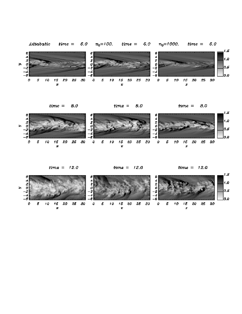
Figure 10: Grey-scale images of the density distribution for equidense ($\nu=1$) adiabatic (left column), and radiative jets, with the product of the jet density and radius $n_{0}a=5\times 10^{17}$ cm^-2 (center column) and $n_{0}a=5\times 10^{18}$ cm^-2 (right column); 2D cuts at a fixed $z$ ($z=0$).

The smallness of the effects introduced by radiation could have been predicted from the analysis of Fig. 9, which shows that the amount of energy lost by radiation is similar to the light jet case, and is smaller by more than an order of magnitude when compared to losses associated with the heavy jet. For this reason, we have examined an additional case with $n_{0}a$ increased by an order of magnitude, i.e., $n_{0}a=5\times 10^{18}$ cm^-2, which is consistent, for example, with a jet radius $a=5\times 10^{15}$ cm and a jet particle density $n_{0}=1000$ cm^-3. This will increase radiative losses; for example, the amount of energy lost by radiation at time $t=8$ corresponds to 0.08% of the kinetic energy of the jet at that same time, compared to a value of 0.02% obtained in the previous case. The results for this high-cooling case are also shown in Fig. 10, in the third column.

Looking at the general evolution, the upper panels of Fig. 10 show that at time $t=6$ shocks have formed, as a consequence of the non-linear growth of the helical mode; the fluting modes drive deformations of the jet surface and entrainment of the external medium by the jet. (Previous times are not represented since $t=6$ is the first time when non-linear effects can be detected.)  The evolution of fluting modes, which are responsible for early mixing, is similar in equal-density jets and in heavy jets, for both adiabatic and radiative cases: however, mixing between the jet and the external medium starts later (at time $t=6$) with respect to the $\nu=0.1$ case. Mixing has an immediate and disruptive effect: external material is entrained and the jet diameter widens quickly; at time $t=12$ the jet maintains its large-scale structure and collimation, but on small scales it appears completely mixed with the ambient medium. Comparing the results for the three cases, we see that the radiative cases show stronger density enhancements inside the jets, and that the widening in the radiative cases is reduced (this reduction is particularly evident in the high-cooling case). This is again confirmed by Fig. 11c), which shows the behavior of the jet radius, as defined above, as a function of time.

As for the heavy jet case, the acoustic and mixing stages cannot be distinguished in the jet evolution, both for the adiabatic and radiative cases. The onset of mixing is contemporary with the formation of the first shocks in the flow, but the interaction of the two phenomena is different if cooling is significant: in the adiabatic and $n_{0}=100$ jets, vigorous mixing takes place and shocks are destroyed after a few sound-crossing times, while in the cooling $n_{0}=1000$ jet strong shocks survive up to the latest stages in the jet evolution, when the global collimation of the jet has been partially destroyed. In fact, in the adiabatic jet a strong shock appears only at time $t=6$, while no shocks survive after time $t=8$ when a weak discontinuity in the flow can be traced. In the cooling $n_{0}=1000$ jet, instead, shock waves are not destroyed up to time $t=14$; this is approximately the time at which the cooling jet enters the quasi-stationary stage of the evolution, as it is indicated by the behavior of the tracer entropy shown in Fig. 11a). Entropy grows more steeply for the adiabatic case: the quasi-stationary phase is attained earlier, i.e., at time $\sim t=12$.

Figure 11: In panel (a) we show a plot of the tracer entropy for the radiative, $n_{0}=100$ (solid line), radiative, $n_{0}=1000$ (dotted line) and adiabatic (dashed line) jets as a function of time; in panel (b) we show a plot of the jet momentum for the radiative, $n_{0}=100$ (solid line), radiative, $n_{0}=1000$ (dotted line) and adiabatic (dashed line) jets as a function of time. In panel (c) the temporal evolution of the jet radius for the radiative, $n_{0}=100$ (solid line) , radiative, $n_{0}=1000$ (dotted line) and adiabatic (dashed line) cases is plotted. All the plots are for the equal density jet case ($\nu=1$).

Fig. 11b) shows the variation in jet momentum as a function of time for the radiative and adiabatic jets. The momentum loss appears to occur slightly faster for the adiabatic and $n_{0}=100$ jets, although the final loss attained at the end of the evolution is similar for the three cases, and corresponds to the $\sim$ 10% of the initial jet momentum. Although the integrated values are similar in all cases, the spatial distribution of the jet momentum reflects the differences in the jet widening noted above.

6 Energy spectra

Table 2: Value of the maximum kinetic energy in the transverse motions, time at which this maximum is reached and time at which equipartition between longitudinal and transverse energy is attained, for all cases, and in four different scale intervals. Blank spaces are left where equipartition was not observed within the maximum evolutionary time reached in our calculations.

	$\lambda<0.5$			$0.5<\lambda<1$			$1<\lambda<2$			$\lambda>2$
	$E_{max}$	$t_{max}$	$t_{eq}$	$E_{max}$	$t_{max}$	$t_{eq}$	$E_{max}$	$t_{max}$	$t_{eq}$	$E_{max}$	$t_{max}$	$t_{eq}$
$\nu=0.1$ - Ad.	$5.5\times 10^{-3}$	$6.$	$9.5$	$6\times 10^{-3}$	$6.$		$6\times 10^{-3}$	$6.$		$1.8\times 10^{-2}$	$6.$
$\nu=0.1$ - Rad.	$5\times 10^{-3}$	$6.$		$5.5\times 10^{-3}$	$6.$		$4.5\times 10^{-3}$	$6.$		$8\times 10^{-3}$	$6.$
$\nu=1.$ - Ad.	$10^{-2}$	$8.1$	$11.5$	$10^{-2}$	$8.5$	$13.$	$10^{-2}$	$8.5$	$14.5$	$2.3\times 10^{-2}$	$10.$
$\nu=1.$ - Rad.	$8.\times 10^{-3}$	$8.1$	$12.5$	$8.\times 10^{-3}$	$8.8$	$14.$	$7.\times 10^{-3}$	$8.8$	$16.$	$1.6\times 10^{-2}$	$10.$
$\nu=10.$ - Ad.	$1.3\times 10^{-2}$	$12.$	$13.2$	$1.3\times 10^{-2}$	$12.$	$16.$	$10^{-2}$	$13.$	$18.$	$2.\times 10^{-2}$	$14.$
$\nu=10.$ Rad.	$10^{-2}$	$12.$	$16.$	$8\times 10^{-3}$	$12.$	$18.5$	$8\times 10^{-3}$	$13.$	$20.$	$1.5\times 10^{-2}$	$14.$

We have seen that radiation losses tend to maintain jet collimation. To obtain a different perspective on the instability evolution and on the differences between the various cases, we have analyzed the relative amounts of kinetic energy in longitudinal and transverse motions at different scales.

When the instability grows, the kinetic energy of the longitudinal jet bulk motion goes into internal energy, radiation, and kinetic energy in the transverse motions. In the direction perpendicular to the jet axis we can have: a) large-scale motions, due to the growth of the helical unstable modes, and b) small-scale motions, induced by the Kelvin-Helmholtz fluting modes, and by a possible turbulent cascade from large to small scale motions. Our aim is to analyze in more detail the transfer of energy from longitudinal to transverse motions; the key issue is to identify possible differences due to radiative losses. This analysis can also give us informations about the persistence of the jet as a coherent structure of longitudinal velocity.

We perform this analysis by calculating the three-dimensional Fourier spectra of the kinetic energy for longitudinal and transverse motions. We then obtain one-dimensional spectra by integrating first over the transversal wavenumbers $k_{y}$ and $k_{z}$, and second over the longitudinal and azimuthal wave numbers (after transforming to cylindrical coordinates). We use these one-dimensional Fourier spectra ${\rm A}_{x}(k_{x})$ and ${\rm A}_{r}(k_{r})$ to compare the amount of energy in the longitudinal and radial direction, at all times, and for all the studied cases. Initially, before the jet enters the non-linear phase, the energy is found in longitudinal motions at large scales; as the instability evolves, a portion of the kinetic energy is transferred to longitudinal motions at smaller scales and to transverse motions. In Fig. 12 we can follow this process for the particular case of underdense jets. The figure shows the behavior of longitudinal and transverse energies, normalized to the initial jet kinetic energy, as a function of time for different scale ranges (recall that lengths are given in units of the jet radius). Looking at the longitudinal energy at large scales ($\lambda>2$, panel a) we see that this component, as noted above, initially represents the only form of energy present in the system and, as the instability evolves, this component decreases monotonically. At smaller scales (panels b,c,d) the longitudinal energy first increases, reaches a maximum, and then decreases. The time at which the maximum is reached is about the same for all the scale ranges. A similar behavior is found for the transverse energy, but the maximum is reached at later times. The faster decrease observed in longitudinal energy when compared to that observed for the transverse energy leads at some time to an equipartition between the two and, from then on, motions can be considered to be isotropic. This isotropy is first reached at small scales, and then at larger scales. We further note, by comparing the curves for the adiabatic case and those for the radiative case, that in this last case the transfer of energy to transverse motions is less efficient and more energy is always kept in longitudinal motions.

The behavior described for the underdense case is found also for the other cases; we have then summarized all our results in Table 2, where we report, for all our cases and for each scale interval, the time at which the maximum of transverse energy is reached, the value of this maximum, and the time at which equipartition between longitudinal and transverse energy is attained.

By comparing the table with the behavior of entropy and momentum shown above, we can see that the time at which the maximum transverse energy is reached falls in the steepest portion of the momentum drop and of the energy growth, confirming the connection between the mixing process and the transfer of energy to the transverse motions. In the case of radiative jets, this process of energy transfer is less efficient as demonstrated by the lower values of $E_{max}$ for these cases and, as discussed above, mixing and jet widening is lower for these types of jets. Comparing the different values of the density ratio, we see that $E_{max}$ increases slightly as $\nu$ is increased, i.e., going from overdense to underdense jets. This increase however cannot compensate for the increase in density with $\nu$; therefore we expect lower transverse velocities for the high $\nu$ cases, and therefore a smaller jet widening, as it is indeed observed in our simulations.

Figure 12: Kinetic energy for longitudinal and transverse motions, as a function of time for light jets. Solid and dotted lines represent the energy of longitudinal motions respectively for adiabatic and radiative jets; dot-dashed and dashed lines represent the energy of transversal motions again for adiabatic and radiative jets.

The table also shows that near the end of our simulations for the $\nu=1$ and $\nu=10$ cases, we reach equipartition between the longitudinal and transverse energies also at scales larger than the jet radius, while in the overdense case equipartition is found only at small scales. We can therefore ask whether, in these cases, the jet can still be identified as a coherent velocity structure. To answer this question, we have computed the autocorrelation function for the longitudinal velocity, defined as

$$F(h)=\int v_{x}(x,y,z)v_{x}(x+h,y,z)dxdydz$$

where the integral is performed over the whole domain of integration. We have then defined a correlation length as

$$l_{c}=\int_{0}^{L}F(h)/F(0)dh$$

and have plotted in Fig. 13 $l_{c}$ as a function of time for all the different cases. The three panels in the figure refer respectively to the overdense case (upper panel), the equal density case (middle panel) and the underdense case (lower panel); the solid curves are for adiabatic cases and the dashed curves are for radiative cases.

Figure 13: Longitudinal velocity autocorrelation length as a function of time, the autocorrelation length is in units of the size of the domain. The upper panel refers to $\nu=0.1$, the middle panel refers to $\nu=1$ and the lower panel refers to $\nu=10$. The solid curves are for the adiabatic cases, while the dashed curves are for the radiative cases.

From Figure 13, we see that, as was also suggested by the Fourier analysis described above, the overdense case maintained an higher coherence than the other two cases, especially compared to the low density case in which $l_{c}$ drops to $\sim 0.4$ at the end of the simulation. Radiation acts in different directions for the different values of $\nu$: in the overdense case radiation tends to give a more inhomogeneous structure both in density (as we have already seen) and in velocity and this is reflected by the lower value of $l_{c}$, in the equal density case the effects of radiation are very small, while in the underdense case radiation tends to keep a more coherent structure with an higher value of $l_{c}$.

7 Summary and Conclusions

We studied the evolution of the Kelvin-Helmholtz instability in three-dimensional jets, solving the hydrodynamical equations through a finite-differences numerical code, adopting a temporal approach and varying the external-to-ambient medium density; we thus considered dense, underdense and iso-dense jets. The main results of our calculations can be summarized as follows:

• Heavy jet

  Dense jets undergo fast evolution. Both helical and fluting modes grow non-linearly at the earliest stages of the evolution, giving rise to large scale deformations in the structure of the jet and to entrainment of ambient material. If cooling is present, the duration of the acoustic phase of the evolution is increased, and shocks survive in the flow for longer times. Furthermore, the strength of the fluting modes is reduced; as a result, mixing with the ambient medium is less effective and the jet retains its collimation for longer times. The momentum loss in the adiabatic and radiative cases is similar, but it occurs in different ways: in both cases, the momentum is transferred away from the jet axis. However, the adiabatic jet loses momentum by expansion and entrainment of ambient medium far from the jet axis, material which is heated and expands by shocks that are driven into the ambient matter from the jet; in contrast, the radiative jet transfers its momentum to ambient material which is located near the jet surface, material which has been shocked and cooled, and thus condensed relative to its initial state.

• Light jet

  For underdense jets the evolution develops over 20 sound crossing times, and thus is slower than the previous case. Mixing takes place later with respect to the onset of the acoustic stage, and its action is damped by the inertia of the external medium. The final jet widening is caused by the growth in amplitude of the fundamental helical mode, which is the main source of shock formation and momentum loss. The amount of energy lost through radiation at a fixed time is smaller than in the previous case, but cooling has nonetheless a small effect on the instability evolution, again reducing the amplitude of the jet widening.

• Equidense jet

  Iso-dense jets evolve similarly to dense jets, although the onset of the various stages is delayed in time. The amount of energy lost through radiation is smaller, and the short duration of the shock-dominated stage suppresses the effects of cooling on the overall instability evolution. To demonstrate the effects of radiative losses, we ran a simulation in which we increased the jet particle density (which is one of the radiative control parameters). The main effects of cooling are a longer duration of shocks in the flow, damping of the helical unstable mode (and thus of the amplitude of the jet deformations in the transverse direction) and of the fluting modes, which implies that mixing is limited to the external layers of the jet.

These results indicate that radiative losses indeed cause jet stabilization, an effect which is more evident in the overdense case and less evident in the other cases; they are thus consistent with the results of previous 2D studies by Rossi et al. (1997) and Micono et al. (1998), even though the effect is not large as in the cases studied by these authors. This difference can be explained as a result of the assumptions of (i) cylindrical geometry with axial symmetry and (ii) axi-symmetric initial perturbations for the 2D cases. The evolution of the instability in two dimensions is then dominated by strong shocks on the jet axis: the amount of energy lost through radiation in these strong compressions is high, and the stabilizing effects of cooling are enhanced. In our 3D study, the strength of the shock waves that form is smaller, both because of geometry and because of small-scale motions driven by the growth of the Kelvin-Helmholtz fluting modes (the latter are neglected in two dimensions). In this way, the effects of cooling are weaker, and their importance depends on the density ratio between the jet and the ambient medium. However, our results can confirm that cooling is efficient in reducing the disruptive action of the instability, in maintaining the jet collimation for longer times, and in extending the temporal duration of the stage where shocks are present in the flow.

Acknowledgments: The calculations have been performed on the Cray T3E at CINECA in Bologna, Italy, thanks to the support of CNAA. This work has been supported in part by and by the DOE ASCI/Alliances grant at the University of Chicago. M.M. acknowledges the CNAA 3/98 grant.

8 References

Birkinshaw, M. ‘Beams and Jets in Astrophysics’ 1991

Bodo, G., Massaglia, S., Ferrari, A., Trussoni, E., 1994, A&A 283, 655

Bodo, G., Massaglia, S., Rossi, P., Rosner, R., Malagoli, A., Ferrari, A., 1995, A&A 303, 281

Bodo, G., Rossi, P., Massaglia, S., Ferrari, A., Malagoli, A., Rosner, R., 1998, A&A 333, 1117

Colella, P., Woodward, P.R., 1984, J. Comp. Phys. 54, 174

Downes, T.P., Ray, T.P., 1998, A&A 331, 1130

Ferrari, A., 1998, Ann.Rev.As.Ap. 36, 539

Gerwin, R.A., 1968, Rev.Mod.Phys. 40, 532

Hardee, P.E., Norman, M.L., 1988, ApJ 334, 70

Hardee, P.E., Clarke, D.A., Howell, D.A., 1995, ApJ 441, 644

Hardee, P.E., Clarke, D.A., 1995, ApJ 451L 25

Hardee, P.E., Clarke, D.A., Rosen, A., 1997, ApJ 485, 533

Hardee, P.E., Stone, J.M., 1997, ApJ 483, 121

Massaglia, S., Trussoni E., Bodo G., Rossi P., Ferrari A. 1992, A&A 260, 243

Micono, M., Massaglia, S., Bodo, G., Rossi, P., Ferrari, A., 1998, A&A 333, 989

Rossi P., Bodo, G., Massaglia, S., Ferrari, A., 1997, A&A 321, 672