Detection of a spectroscopic transit by the planet orbiting the star HD209458

Abstract

We report the first detection of a planetary transit by spectroscopic measurements. We have detected the distortion of the stellar line profiles during a planetary transit. With the ELODIE spectrograph we took a sequence of high precision radial velocities of the star HD209458 at time of a transit of its planet. We detected an anomaly in the residuals of the orbit. The shape and the amplitude of the anomaly are modeled as a change of the mean stellar line profile resulting from the planet crossing the disk of the rotating star. The planetary orbit is in the same direction as the stellar rotation. Using the photometric transit to constrain the timing and the impact parameters of the transit, we measure an angle $\alpha=3.9$ [⁰] between the orbital plane and the apparent equatorial plane as well as a $v\sin i$=$3.75\pm 1.25$ km s^-1. With additional constrains on the inclination of the star and on the statistics of the line of sight distribution, we can set an upper limit of 30 ⁰ to the angle between the orbital plane and the stellar equatorial plane.

1 Introduction

A Jupiter mass companion having a short period orbit was recently detected for the star HD209458 by high-precision radial velocity surveys (Henry et al. (2000), Mazeh et al. (2000)). Luckily, the orbital plane of the planet is close enough to the line of sight for transits to occur and be detected by photometric measurements (Charbonneau et al. (2000), Henry et al. (2000)). The measurement of the photometric transit across HD209458 is the first independent confirmation of the reality of the giant planets in short period orbits detected by radial velocity surveys (see Marcy et al. (1999) for a review). It leads to the first estimate of the radius of a ”hot Jupiter” planet (or 51-Peg type planet) and it strongly constrains the orbital inclination $i_{\hbox{\scriptsize orb}}$.

The crossing of a companion in front of a rotating star produces a change in the line profile of the stellar spectrum. During its transit across the star, the companion occults a small area of the stellar disk. If the star is rotating, the stellar line profiles will be distorted according to the location of the planet in front of the stellar disk. This phenomenon was already well known from past observations of eclipsing binaries. It was first detected on $\beta$ Lyrae and Algol systems by Rossiter (1924) and McLaughlin (1924). Recently, it has been suggested by Schneider (2000) that a transit by a planet could also be detected in the line profile of high signal-to-noise ratio stellar spectra for stars with high $v\sin i$. But most of the stars with a close-in planet have low $v\sin i$  values and in such a case the line profile distortion by a transit would be less than 1% of the width of the lines. This small effect is extremely challenging to detect for individual lines, but if a multi-line approach – like in the cross-correlation technique – is used, the mean effect could be large enough to be measured. Actually, any slight distortion of the stellar line profile changes the radial velocity measured from the Doppler effect, similar to the effect of stellar spots on rotating stars (see Queloz (1999) for references and details). Current high-precision radial velocity measurements probably offer the easiest way to detect a spectroscopic transit of a giant planet.

The timing and the amplitude of the drop of the stellar luminosity observed during a planetary transit measure the radius of the planet and its orbital inclination to the line of sight. The detection of a spectroscopic transit by radial velocity measurements provides a unique means to estimate the relative inclination ($\alpha$) between the stellar equatorial plane projected on the line of sight (called hereafter the apparent equatorial plane) and the orbital plane, as well as the ascending node of the orbit ($\Omega_{p}$) on the apparent equatorial plane.

From a weak friction model (Hut (1981)) we find that the tidal effect of a short period Jupiter-mass planet on the star is not strong enough to force coplanarity. Comparison between the coplanarization time and the stellar circularization time indicates that the alignment time is 100 times longer than the circularization time. The stellar circularization time is of the order of a billion years (Rasio et al. (1996)). Usually one makes the assumption that the orbital plane is coplanar with the stellar equatorial plane for close-in planets. Combined with the $v\sin i$  measurement of the star, this ad-hoc assumption is used to set an upper limit to the mass of the planet (e.g. Mayor & Queloz (1995)). The shape of the radial velocity anomaly during the transit provides a tool to test this hypothesis. Moreover, the coplanarity measurement is also a way to test the formation scenario of 51-Peg type planets. If the close-in planets are the outcome of extensive orbital migration, we may expect the orbital plane to be identical to the stellar equatorial plane. If other mechanisms such as gravitational scattering played a role, the coplanarity is not expected. A review of formation mechanisms of close-in planets may be found in Weidenschilling & Mazzari (1996) and Lin et al. (1999).

The amplitude of the radial velocity anomaly stemming from the transit is strongly dependent on the star’s $v\sin i$  for a given planet radius. A transit across a star with high $v\sin i$  produces a larger radial velocity signature than across a slow rotator. However it is more difficult to measure accurate radial velocities for stars with high $v\sin i$. It requires higher signal-to-noise spectra because the line contrast is weaker. A star like HD209458 with $v\sin i$  about 4 km s^-1  is a good candidate for such a detection. With the large wavelength domain of ELODIE (3000Å) approximately 2000 lines are available for the cross-correlation thus only moderate signal-to-noise ratio spectra (50-100) are required.

If we use the planet’s radius derived from the photometric transit, the $v\sin i$  of the star can be estimated from the measurement of the spectroscopic transit. Unlike spectral analysis, the measurement of the $v\sin i$  provided by the spectroscopic transit is almost independent of the accurate knowledge of the amplitude of the spectral broadening mechanism intrinsic to the star. A complete description of transit measurements is given in Kopal (1959) for eclipsing binaries and Eggenberger et al. (in prep.) for planetary transit cases.

2 The measurement of the spectroscopic transit

During the transit, on November 25th 1999, we got a continuous sequence of 15 high precision radial velocity measurements with the spectrograph ELODIE on the 193cm telescope of the Observatoire de Haute Provence (Baranne et al. (1996)) using the simultaneous thorium setup. The following night we repeated the same sequence, but off-transit this time, in order to check for any instrumental systematics possibly stemming from the relative low position on the horizon. For both nights the sequence was stopped when a value of two airmasses was reached. The ADC (atmospheric dispersion corrector) does not correct efficiently at higher airmass.

As usual for ELODIE measurements, the data reduction was made on-line at the telescope. The radial velocities have been measured by a cross-correlation technique with our standard binary mask and Gaussian fits of the cross-correlation functions (or mean profiles) (see Baranne et al. (1996) for details).

Figure 1: Two sequences of radial velocity residuals for the star HD209458 taken at the same time during the night but one day apart. The data are corrected for the orbital motion of the planet with the Mazeh et al. (2000) ephemeris. Top out of the planetary transit, the residuals agree with random error. Bottom during the planet transit an anomaly is detected. The duration of the photometric transit is indicated by the thick dashed line. Notice the good timing agreement between the beginning of the photometric transit and the beginning of the radial velocity anomaly. Our best model of the radial velocity anomaly (see below) is superimposed on the data (solid line). The $1\sigma$ confidence level of the anomaly model is illustrated by the dotted area

The residuals from the spectroscopic orbit of HD 209458 (Mazeh et al. (2000)) are displayed for two selected time spans in Fig. 1. During the transit an anomaly is observed in the residuals. The probability to be a statistical effect of a random noise distribution is $10^{-4}$ ($\chi 2=53.4$). The second night with the same timing sequence no significant deviation from random residuals is observed. Note that the usual 10 m s^-1long-term instrumental error has not been added to the photon-noise error since the instrumental error is negligible on this time scale, accordingly with the 40% confidence level measured for the non-signal model during the off-transit night.

3 Modeling the data

In Fig. 2 the geometry of our model is illustrated. The orbital motion is set in the same direction as the stellar rotation. This configuration actually stems from the transit data themselves: the radial velocity anomaly first has a positive bump and then a negative dip. This tells us that the planetary orbit and the stellar rotation share the same direction whatever the geometry of the crossing may be (direct orbit).

Figure 2: Illustration of the geometry of our model. The $(x-y)$ plane is called apparent equatorial plane. The y-axis is the line of sight. Notice the definition of the angle $\alpha$ and the ascending node $\Omega_{p}$ on the apparent equatorial plane. The angle between the star’s equatorial plane and the planetary plane is described by $\psi$. On the $(x-z)$ plane the thick line represents the orbital trajectory projected on the stellar disk. The stellar rotation axis (dashed line) is seen in the plane $(y-z)$ with its angle $i$.

In this paper we decided to restrict our analysis to the measurement of three parameters: the angle $\alpha$ between the orbital plane and the apparent equatorial plane, the $v\sin i$  of the star and the ascending node $\Omega_{p}$. The ascending node is taken positive in the direction of the star’s rotation and equal to $90^{0}$ when crossing the line of sight axis. The timing of the transit and the impact parameter $\Delta$ (shorter projected distance between the transit trajectory and the star center) are set by the results of the photometric transit. The Hipparcos measurements of the transit (Robichon & Arenou (2000)) constraint a very accurate orbital period of the system. Combined with the mid-time of the transit by Mazeh et al. (2000), we know the observed transit mid-time with an accuracy of 5 minutes. More radial velocity data at high precision would be required to make a full adjustment of the transit (timing and geometry). In Table 1 we list the results from the spectroscopic orbit and the photometric transit that were used to constrain our model adjustments.

Table 1: Star, planet and orbit parameters of our model

fixed parameters
$P$		$3.524739\pm 1.4\cdot 10^{-5}$ d
$a$		$0.047\pm 0.001$ AU
$e$		$0$
$T_{c}^{\diamond}$		$2451508.368\pm 0.0032$
$R_{\star}$		1.2($\pm 0.1$) R⊙
$R_{\hbox{\scriptsize\rm planet}}$		1.40($\pm 0.17$) RJ
$\Delta^{\ddagger}$		$0.569\pm 0.004$ R⋆
Our best solution
$v\sin i$		$3.75\pm 1.25$  km s-1
$\alpha$		$\pm 3.9^{+18}_{-21}$ [0]
$\Omega_{p}^{\dagger}$	for $\alpha=3.9$	$0$ [0]
	for $\alpha=22$	$100$ [0]
	for $\alpha=-25$	$81$ [0]

Orbit and transit data are from Mazeh et al. (2000) excepted for the period which is from Robichon & Arenou (2000)
(^⋄) computed with $P$ of Robichon & Arenou (2000) and $T_{c}$ by Mazeh et al. (2000)
(^‡) derived from the orbital inclination angle $86.1^{0}\pm 1.6^{0}$
(^†) $\pm 180$ [⁰] undefined

In our model we consider a spherical star in uniform rotation. The star is divided into 90000 cells. A Gaussian shape cross-correlation model with $\sigma_{0}=3.0$ km s^-1width is used to model the mean individual spectral line of each cell where the center of the Gaussian is equal to the mean radial velocity of the cell. The effect of the $\sigma_{0}$ value on the $v\sin i$  estimate is negligible: with $\sigma_{0}=2.5$ km s^-1  we would only increase the $v\sin i$  measurement by 0.1 km s^-1.

The integration is made by summation of the cells free of the planet along the line of sight. A linear limb darkening weighting ($B_{\mu}=1-\epsilon(1-\mu)$) with $\epsilon=0.6$ is used in the sum. The planetary orbit is circular. We divide the transit into 50 phase steps for computing the radial velocity anomaly of the spectroscopic orbit residuals.

To illustrate the effect of the transit geometry on the radial velocity anomaly during the transit, we display in Fig. 3 the anomaly expected for three geometric configurations and two different $v\sin i$  values. We see that the amplitude of the anomaly is driven by the $v\sin i$  value of the star. The radial-velocity symmetry of the anomaly of the spectroscopic orbit residuals (from the mid-transit) for $\Delta>0$ impact parameter depends on the angle $\alpha$ between the stellar apparent equatorial plane and the orbital plane. Interestingly enough, the $\alpha$ parameter is not tied to the $v\sin i$  measurement. The two parameters are uncorrelated. In Fig. 3 we also see that the mirror trajectories along the apparent equatorial plane make similar radial velocity anomalies because $\Omega_{p}$ is $\pm 180$ [⁰] undefined. Nevertheless, the value of $\Omega_{p}$ can be used to make the distinction between cases a and b from Fig. 3.

Figure 3: Illustration of the effect of the geometry of the transit on the radial velocity anomaly for HD209458: Upper panel. Geometry of the crossing for 3 cases (+3 symmetrical cases): (a) $\alpha=20$ [⁰] and $\Omega_{p}\in[0;90]\cup[180;270]$; (b) $\alpha=20$ [⁰] and $\Omega_{p}\in[90;180]\cup[270;360]$; (c) $\alpha=3.9$ [⁰] (horizontal trajectory). Lower Panel. Radial velocity anomalies for the geometries displayed above for (top) $v\sin i$=3 km s^-1and (bottom) $v\sin i$=4.75 km s^-1

The comparison of the transit model with the data is made by $\chi^{2}$ statistics with the velocity offset, the star’s $v\sin i$, and $\alpha$ as free parameters. To distinguish the geometry of the two trajectories that have similar $\alpha$ angle but different $\Omega_{p}$ value, we arbitrarily set $\alpha<0$ when $\Omega_{p}$ value is between 0 and 90 (or 180-270) and $\alpha>0$ when $\Omega_{p}$ value is between 90 and 180 (or 270-360). These are respectively the a and b trajectories illustrated on Fig. 3.

The best set of $\alpha$-$v\sin i$  solutions is listed in Table. 1 with $1\sigma$ confidence levels. Following our definition of $\alpha$, any angle with $3.9<\alpha<-3.9$ [⁰] is impossible given our impact parameter $\Delta=0.569$ R_⋆. Our best fit is reached when $\alpha=\pm 3.9$ and $\Omega_{p}=0$. It corresponds to a transit trajectory parallel to the apparent equatorial plane.

The uncertainties on our best solution listed in Table. 1 do not include systematics stemming from errors in fixed parameters of the model. A ($\pm 0.17\,R_{J}$) change of the planet radius would lead to a change of the $v\sin i$  by $\pm$0.75 km s^-1. Actually if the planet has indeed a larger radius we overestimate the $v\sin i$  value. The uncertainty on the star radius has a weaker effect on the $v\sin i$  measurement than the uncertainty on the planet radius. A change of the star radius by $\pm 0.1\,R_{\odot}$ would make the $v\sin i$  change by 0.3 km s^-1only.

4 Discussion

We have successfully demonstrated the detection of a planetary transit using a time sequence of stellar spectra when the stellar line profile is distorted by the crossing of the planet and changes the radial velocity measurement of the star. We have detected an anomaly in the residuals of the radial velocity orbit of HD 209458 at the time of the transit. This anomaly has been modeled with high confidence as the effect of the planetary transit. The data suggest an orbital trajectory parallel to the apparent equatorial plane.

The measurement of an $\alpha$ different from zero and an ascending node off the plane of the sky ($\Omega_{p}\neq 0$) would indicate deviation from the coplanarity between the orbital plane and the stellar equatorial plane. In our case we can only argue that no evidence for non-coplanarity is found. However additional arguments can set some limits on the coplanarity level. From the statistics only, it would be ”bad luck” to observe a non-coplanar system in a configuration such as $\alpha\approx 0$ and $\Omega_{p}=0$. This would only happen for a very small set of system orientations. We computed the probability of finding $\alpha$ smaller than $\alpha_{max}$ for a system with an angle $\psi$ between its orbital plane and the equatorial plane (see on Fig. 2 for an illustration of the $\psi$ angle). First, we have determined the relation between $\alpha$ and $i$ for various $\psi$ configurations. Simply said we have computed for each configuration all the different spectroscopic signals that extra-terrestrial observers looking at the system from different points of view could see the same photometric transit. Then we have generated series of random numbers $i$ by recalling that the probability of seeing a system with a small $i$ is smaller than the probability of seeing a system with a large $i$. For each of these values we have used the relation between $\alpha$ and $i$ to calculate the corresponding statistical distribution of $\alpha$. Finally the cumulative distribution of $\alpha$ is shown on Fig. 4. With $1\sigma$ confidence level we can rule out a $\psi$ angle larger than 30 degrees.

To get a complete description of the coplanarity between the stellar equatorial plane and the orbital plane, measurement of the angle $i$ is required. Ideally $i$ can be estimated from the rotation rate of the star. HD209458 has a quiet chromosphere ($R_{HK}=-4.9$ by Henry et al. (2000)) but significant spectral line rotation broadening ($v\sin i$) is detected. The spectroscopic $v\sin i$  measurements have a weighted mean value of $3.7\pm 0.5$  km s^-1(measurements by Mazeh et al. (2000) and Marcy et al. private comm.) in agreement with the value measured in this work. The low chromospheric HK value suggests a rotation period of at least 17 days (Noyes et al., (1984)). With the $v\sin i$  and the period estimate we find $i\tilde{>}60^{0}$.

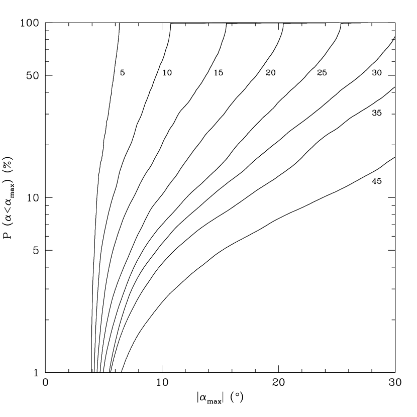
Figure 4: Probability to measure an angle $\alpha$ for various configurations. The labels of curves describes the angle $\psi$ (⁰) between the equatorial plane and the orbital plane

The statistical result on the geometry distribution of the system added to the constraint on $i$ provides two arguments refuting strong non-coplanarity for this system. Better measurements of the spectroscopic transit are needed to get stronger constrains. Simulations show that for a coplanar system with the same radial velocity accuracy but 4 times more data spread over the whole transit duration, the error bars on the measurement of $\alpha$ would be small enough to conclude that $\psi<10[^{0}]$ with $1\sigma$ confidence level.