Accepted for publication in Monthly Notices
Formulae for Growth Factors In Expanding Universes Containing Matter and a Cosmological Constant

Abstract

Formulae are presented for the linear growth factor $D/a$ and its logarithmic derivative ${\rm d}\ln D/{\rm d}\ln a$ in expanding Friedmann-Robertson-Walker Universes with arbitrary matter and vacuum densities. The formulae permit rapid and stable numerical evaluation. A fortran program is available at http://casa.colorado.edu/$\sim$ajsh/growl/.

1 Introduction

The linear growth factor $g\equiv{D/a}$, where $D$ is the amplitude of the growing mode and $a$ is the cosmic scale factor, determines the normalization of the amplitude of fluctuations in Large Scale Structure (LSS) relative to those in the Cosmic Microwave Background (CMB) (Eisenstein, Hu & Tegmark 1999 Appendix B.2.2). Its logarithmic derivative, the dimensionless linear growth rate $f\equiv{\rm d}\ln D/{\rm d}\ln a$, determines the amplitude of peculiar velocity flows and redshift distortions (Peebles 1980 §14; Willick 2000; Hamilton 1998). As such, the growth factor $g$ and growth rate $f$ are of basic importance in connecting theory and observations of LSS and the CMB.

In a Friedmann-Robertson-Walker (FRW) Universe containing only matter and vacuum energy, with densities $\Omega_{\rm m}$ and $\Omega_{\Lambda}$ relative to the critical density, the linear growth factor is given by (Heath 1977; Peebles 1980 §10)

$$g(\Omega_{\rm m},\Omega_{\Lambda})\equiv{D\over a}={5\,\Omega_{\rm m}\over 2}\int_{0}^{1}{{\rm d}a\over a^{3}H(a)^{3}}\ ,$$ (1)

where $a$ is the cosmic scale factor normalized to unity at the epoch of interest, $H(a)$ is the Hubble parameter normalized to unity at $a=1$,

$$H(a)=\left(\Omega_{\rm m}a^{-3}+\Omega_{\rm k}a^{-2}+\Omega_{\Lambda}\right)^{1/2}\ ,$$ (2)

and the curvature density $\Omega_{\rm k}$ is defined to be the density deficit

$$\Omega_{\rm k}\equiv 1-\Omega_{\rm m}-\Omega_{\Lambda}\ ,$$ (3)

which is respectively positive, zero, and negative in open, flat, and closed Universes. The normalization factor of $5\,\Omega_{\rm m}/2$ in equation (1) ensures that $g\rightarrow 1$ as $a\rightarrow 0$. It follows from equation (1) that the dimensionless linear growth rate $f$ is related to the growth factor $g$ by

$$f(\Omega_{\rm m},\Omega_{\Lambda})\equiv{{\rm d}\ln D\over{\rm d}\ln a}=\mbox{}-1-{\Omega_{\rm m}\over 2}+\Omega_{\Lambda}+{5\,\Omega_{\rm m}\over 2\,g}\ .$$ (4)

The fact that the integrand on the right hand side of equation (1) is a rational function of the square root of a cubic implies that the integral can be written analytically in terms of elliptic functions. However, the analytic expressions are complicated, and have yet to be implemented in any published code. Explicit analytic expressions in the special case of a flat Universe, $\Omega_{\rm k}=0$, have been given in terms of the incomplete Beta function by Bildhauer, Buchert & Kasai (1992) and in terms of the hypergeometric function by Matsubara (1995). Analytic expressions for the luminosity distance in the general non-flat case are given in terms of elliptic functions by Kantowski, Kao & Thomas (2000).

Lahav et al. (1991) give a simple and widely used approximation to the growth rate:

$$f(\Omega_{\rm m},\Omega_{\Lambda})\approx\Omega_{\rm m}^{4/7}+(1+\Omega_{\rm m}/2)\,\Omega_{\Lambda}/70\ .$$ (5)

From this, together with relation (4), follows the approximate expression for the growth factor quoted by Carroll, Press and Turner (1992):

$$g(\Omega_{\rm m},\Omega_{\Lambda})\approx{5\,\Omega_{\rm m}\over 2\,\left[\Omega_{\rm m}^{4/7}-\Omega_{\Lambda}+(1+\Omega_{\rm m}/2)(1+\Omega_{\Lambda}/70)\right]}\ .$$ (6)

Given the increasing precision of measurements of fluctuations in the CMB (de Bernardis et al. 2000; Hanany et al. 2000) and LSS (Gunn & Weinberg 1995; York et al. 2000; Colless 2000) and the growing evidence favouring a cosmological constant (Gunn & Tinsley 1975; Perlmutter et al. 1999; Riess et al. 1998; Kirshner 1999), it seems timely to present exact expressions, suitable for numerical evaluation, for the growth factor $g$ (hence $f$, through formula [4]) valid for arbitrary values of the cosmological densities $\Omega_{\rm m}$ in matter and $\Omega_{\Lambda}$ in vacuum.

The procedure presented in this paper is to expand the integral of equation (1) as a convergent series of incomplete Beta functions, conventionally defined by

$$B(x,a,b)\equiv\int_{0}^{x}t^{a-1}(1-t)^{b-1}\,{\rm d}t\ .$$ (7)

In effect, the method can be regarded as generalizing Bildhauer et al.’s (1992) formula. What makes the scheme attractive is that the Beta functions in successive terms of the series can be evaluated recursively from each other through the recursion relations

$$a\,B(x,a,b)=x^{a}(1-x)^{b}+(a+b)\,B(x,a+1,b)$$ (8)

$$b\,B(x,a,b)=-x^{a}(1-x)^{b}+(a+b)\,B(x,a,b+1)$$ (9)

$$a\,B(x,a,b+1)=x^{a}(1-x)^{b}+b\,B(x,a+1,b)$$ (10)

the last of which follows from the other two. In practice, each evaluation of the growth factor $g$ involves from one to seven calls to an incomplete Beta function, followed by elementary recursive operations.

The resulting numerical algorithm is fast (provided that $\Omega_{\rm m}$ and $|\Omega_{\Lambda}|$ are not huge – see §3) and stable, and has been implemented in a fortran package grow$\lambda$ available at http://casa.colorado.edu/$\sim$ajsh/growl/. The grow$\lambda$ package includes an updated version of an incomplete Beta function originally written by the author a decade ago.

2 Formulae

Figure 1 shows contour plots of the growth factor $g(\Omega_{\rm m},\Omega_{\Lambda})$ and growth rate $f(\Omega_{\rm m},\Omega_{\Lambda})$ computed from the formulae presented below, as implemented in the code grow$\lambda$. The results have been checked against numerical integrations with the Mathematica program.

Perhaps the most striking aspect of these plots, emphasized by Lahav et al. (1991), is that the growth rate $f$ is sensitive mainly to $\Omega_{\rm m}$, with only a weak dependence on $\Omega_{\Lambda}$.

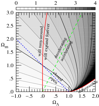
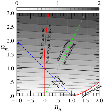
Figure 1: Contour plots of (left) the growth factor $g(\Omega_{\rm m},\Omega_{\Lambda})$, and (right) the growth rate $f(\Omega_{\rm m},\Omega_{\Lambda})$, in expanding Universes containing matter and cosmological constant with densities $\Omega_{\rm m}$ and $\Omega_{\Lambda}$ relative to the critical density. Universes below the $45^{\circ}$ dashed line are geometrically open, while those above are closed. Universes to the upper left of the long dashed line are decelerating, while those to lower right are accelerating. Universes to the left of the almost vertical line near $\Omega_{\Lambda}\approx 0$ will eventually turn around, while Universes to the right will expand forever. The region at the bottom right corner is physically inaccessible to Universes that expand from zero and that contain only matter and cosmological constant. The boundary between turnaround and eternal expansion, and the boundary of the inaccessible region, together form, in the closed case, the approaching and receding parts of the loiter line. Starting at $\Omega_{\rm m}=1$, $\Omega_{\Lambda}=0$, a Universe can evolve upward and rightward along the approaching part of the loiter line to Einstein’s loiter point at $\Omega_{\rm m}=2\,\Omega_{\Lambda}\rightarrow\infty$. After an indefinite period of hanging around, the Universe can then either recollapse along the same loiter line, or else continue into renewed expansion downward and leftward along the receding part of the loiter line, the boundary of the inaccessible region. The growth factor $g$ tends to infinity at the boundary of the inaccessible region, but only contours up to $g=5$ are marked. The contour plot of $g(\Omega_{\rm m},\Omega_{\Lambda})$ is similar to Figure 7 of Carroll et al. (1992).

Figure 2 shows the ratio of the Lahav et al. (1991) growth rate $f$, equation (5), to the true growth rate. The Figure illustrates that the Lahav et al. approximation works well except at small $\Omega_{\rm m}$. The approximation (with the $4/7$ exponent advocated by Lightman & Schechter 1990) works particularly well for currently favoured cosmologies, being accurate to better than $1\%$ for flat Universes with $\Omega_{\rm m}=0.2$–$3.9$.

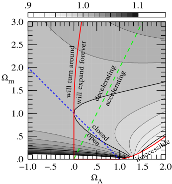
Figure 2: Contour plot of the ratio of the Lahav et al. (1991) growth rate $f$, equation (5), to the true growth rate. The plot illustrates that the Lahav et al. approximation works well except for small $\Omega_{\rm m}$. In particular, the approximation is accurate to better than 1% for currently favoured cosmologies, flat Universes ($45^{\circ}$ dashed line) with $\Omega_{\rm m}\geq 0.2$. For small $\Omega_{\rm m}$ (and any $\Omega_{\Lambda}$) a somewhat better approximation results if the Lightman & Schechter (1990) exponent $4/7$ in equation (5) is replaced with $0.6$, as in Lahav et al.’s original paper. The white region in the diagram at $\Omega_{\rm m}\la 0.1$ and $\Omega_{\Lambda}<1$ is where the error in the Lahav et al. approximation (with the $4/7$ exponent) exceeds 10%; contours in this region are omitted to avoid confusion.

2.1 Limiting cases

The requirement that the Hubble parameter $H(a)$, equation (2), be the square root of a positive quantity for all $a$ from 0 (Big Bang) to 1 (now) imposes two requirements. The first is that the matter density be positive

$$\Omega_{\rm m}\geq 0\ ,$$ (11)

and the second can be interpreted as a condition that the Universe not be too closed

$$\Omega_{\rm k}\geq\min\left[-{3\,\Omega_{\rm m}\over 2},-\left({27\,\Omega_{\rm m}^{2}\Omega_{\Lambda}\over 4}\right)^{1/3}\right]\ .$$ (12)

If either of the two conditions (11) or (12) were violated, then the Hubble parameter $H(a)$ would go to zero at some finite cosmic scale factor $a$, indicating that the Universe did not expand from $a=0$, but turned around from a collapsing to an expanding phase at some finite $a$.

The limiting values of the growth factor $g$ and growth rate $f$ as the matter density goes zero, $\Omega_{\rm m}\rightarrow 0$, are

$$g(\Omega_{\rm m}=0,\Omega_{\Lambda})=0\ ,\quad f(\Omega_{\rm m}=0,\Omega_{\Lambda})=0$$ (13)

provided also that $\Omega_{\Lambda}<1$, in accordance with the condition $\Omega_{\rm k}>0$ from equation (12). Physically, structure cannot grow in a Universe containing only vacuum.

The second condition, equation (12), is saturated when $\Omega_{\rm k}\rightarrow-(27\,\Omega_{\rm m}^{2}\Omega_{\Lambda}/4)^{1/3}$ with $\Omega_{\rm k}<-3\,\Omega_{\rm m}/2$. This marks the boundary of the inaccessible region to the bottom right of Figure 1. The limiting values of the growth factor $g$ and growth rate $f$ in this case are

$$g(\Omega_{\rm m},\Omega_{\Lambda})\rightarrow\infty\ ,\quad f(\Omega_{\rm m},\Omega_{\Lambda})=\mbox{}-1-{\Omega_{\rm m}\over 2}+\Omega_{\Lambda}\ .$$ (14)

Physically, the growth factor tends to infinity because such Universes are in renewed expansion after having spent an indefinite period of time at Einstein’s unstable loitering point, at $\Omega_{\rm m}=2\,\Omega_{\Lambda}\rightarrow\infty$.

2.2 Case $|\Omega_{\rm k}/(1-\Omega_{\rm k})|\leq 1$

For small curvature density $\Omega_{\rm k}$, expand the integral in equation (1) as a power series in $\Omega_{\rm k}$:

$$g(\Omega_{\rm m},\Omega_{\Lambda})={5\,\Omega_{\rm m}\over 2}\int_{0}^{1}{{\rm d}a\over a^{3}(\Omega_{\rm m}a^{-3}+\Omega_{\Lambda})^{3/2}}\sum_{n=0}^{\infty}{(-)^{n}(3/2)_{n}\over n!}\left({\Omega_{\rm k}a^{-2}\over\Omega_{\rm m}a^{-3}+\Omega_{\Lambda}}\right)^{n}$$ (15)

where $(x)_{n}\equiv x(x+1)...(x+n-1)$ is a Pochhammer symbol.

Each term of the sum on the right hand side of equation (15) integrates to an incomplete Beta function. The cases of positive and negative cosmological constant must be distinguished. For positive cosmological constant, $\Omega_{\Lambda}>0$,

$$g(\Omega_{\rm m},\Omega_{\Lambda})={5\,\Omega_{\rm m}^{1/3}\over 6\,\Omega_{\Lambda}^{5/6}}\sum_{n=0}^{\infty}{(-)^{n}(3/2)_{n}\over n!}\left({\Omega_{\rm k}\over\Omega_{\rm m}^{2/3}\Omega_{\Lambda}^{1/3}}\right)^{n}B\left({\Omega_{\Lambda}\over\Omega_{\rm m}+\Omega_{\Lambda}},{5\over 6}+{n\over 3},{2\over 3}+{2n\over 3}\right)\ ,$$ (16)

while for negative cosmological constant, $\Omega_{\Lambda}<0$,

$$g(\Omega_{\rm m},\Omega_{\Lambda})={5\,\Omega_{\rm m}^{1/3}\over 6\,|\Omega_{\Lambda}|^{5/6}}\sum_{n=0}^{\infty}{(-)^{n}(3/2)_{n}\over n!}\left({\Omega_{\rm k}\over\Omega_{\rm m}^{2/3}|\Omega_{\Lambda}|^{1/3}}\right)^{n}B\left({|\Omega_{\Lambda}|\over\Omega_{\rm m}},{5\over 6}+{n\over 3},-{1\over 2}-n\right)\ .$$ (17)

In each of formulae (16) and (17), incomplete Beta functions must be evaluated for three terms, and then the remaining Beta functions can be evaluated recursively from these three, through the recursion relations (8)–(10). In equation (16) ($\Omega_{\Lambda}>0$), the recursion is stable from $n=0$ upward, or from large $n$ downward, according to whether the argument $\Omega_{\Lambda}/(\Omega_{\rm m}+\Omega_{\Lambda})$ is greater than or less than $1/3$. In equation (17) ($\Omega_{\Lambda}<0$), the recursion is stable from $n=0$ upward or large $n$ downward as the argument $|\Omega_{\Lambda}|/\Omega_{\rm m}$ is greater or less than $1+(3/2)[(\sqrt{2}-1)^{1/3}-(\sqrt{2}-1)^{-1/3}]=0.106$.

How fast do the expansions (16) and (17) converge? Convergence is determined essentially by the convergence of the parent expression (15) at the place where the expansion variable $\Omega_{\rm k}a^{-2}/(\Omega_{\rm m}a^{-3}+\Omega_{\Lambda})$ attains its largest absolute magnitude over the integration range $a\in[0,1]$. For $\Omega_{\Lambda}>0$, the expansion variable attains its largest magnitude at $a=\min\{1,[\Omega_{\rm m}/(2\,\Omega_{\Lambda})]^{1/3}\}$, while for $\Omega_{\Lambda}<0$, the expansion variable is always largest at $a=1$. Physically, the extremum at $\Omega_{\rm m}a^{-3}=2\,\Omega_{\Lambda}$ occurs where the Universe transitions from decelerating to accelerating. It follows that if $\Omega_{\rm m}\geq 2\,\Omega_{\Lambda}$ (decelerating), then successive terms of the expansions (16) and (17) decrease by $\approx\Omega_{\rm k}/(\Omega_{\rm m}+\Omega_{\Lambda})$, whereas if $\Omega_{\rm m}\leq 2\,\Omega_{\Lambda}$ (accelerating), then successive terms decrease by $\approx 2^{2/3}\Omega_{\rm k}/(3\,\Omega_{\rm m}^{2/3}\Omega_{\Lambda}^{1/3})$. Thus $n$ terms of the expansions (16) and (17) will yield a precision of $\approx[\Omega_{\rm k}/(\Omega_{\rm m}+\Omega_{\Lambda})]^{n}$ if $\Omega_{\rm m}\geq 2\,\Omega_{\Lambda}$, or a precision of $\approx[2^{2/3}\Omega_{\rm k}/(3\,\Omega_{\rm m}^{2/3}\Omega_{\Lambda}^{1/3})]^{n}$ if $\Omega_{\rm m}\leq 2\,\Omega_{\Lambda}$.

2.3 Case $|\Omega_{\Lambda}/(1-\Omega_{\Lambda})|\leq 1$

For small cosmological constant $\Omega_{\Lambda}$, expand the integral in equation (1) as a power series in $\Omega_{\Lambda}$:

$$g(\Omega_{\rm m},\Omega_{\Lambda})={5\,\Omega_{\rm m}\over 2}\int_{0}^{1}{{\rm d}a\over a^{3}(\Omega_{\rm m}a^{-3}+\Omega_{\rm k}a^{-2})^{3/2}}\sum_{n=0}^{\infty}{(-)^{n}(3/2)_{n}\over n!}\left({\Omega_{\Lambda}\over\Omega_{\rm m}a^{-3}+\Omega_{\rm k}a^{-2}}\right)^{n}\ .$$ (18)

Again, each term of the sum on the right hand side of equation (18) integrates to an incomplete Beta function. The cases of positive and negative curvature density $\Omega_{\rm k}$ must be distinguished. For an open Universe, $\Omega_{\rm k}>0$,

$$g(\Omega_{\rm m},\Omega_{\Lambda})={5\,\Omega_{\rm m}^{2}\over 2\,\Omega_{\rm k}^{5/2}}\sum_{n=0}^{\infty}{(-)^{n}(3/2)_{n}\over n!}\left({\Omega_{\rm m}^{2}\Omega_{\Lambda}\over\Omega_{\rm k}^{3}}\right)^{n}B\left({\Omega_{\rm k}\over\Omega_{\rm m}+\Omega_{\rm k}},{5\over 2}+3n,-1-2n\right)\ ,$$ (19)

while for a closed Universe, $\Omega_{\rm k}<0$,

$$g(\Omega_{\rm m},\Omega_{\Lambda})={5\,\Omega_{\rm m}^{2}\over 2\,|\Omega_{\rm k}|^{5/2}}\sum_{n=0}^{\infty}{(-)^{n}(3/2)_{n}\over n!}\left({\Omega_{\rm m}^{2}\Omega_{\Lambda}\over|\Omega_{\rm k}|^{3}}\right)^{n}B\left({|\Omega_{\rm k}|\over\Omega_{\rm m}},{5\over 2}+3n,-{1\over 2}-n\right)\ .$$ (20)

Here the Beta functions in successive terms can be computed recursively from a single Beta function. In equation (19) ($\Omega_{\rm k}>0)$, the recursion is stable from $n=0$ upward or large $n$ downward as the argument $\Omega_{\rm k}/(\Omega_{\rm m}+\Omega_{\rm k})$ is greater than or less than $3/4$. In equation (20) ($\Omega_{\rm k}<0$), the recursion is stable from $n=0$ upward or large $n$ downward as the argument $|\Omega_{\rm k}|/\Omega_{\rm m}$ is greater than or less than $(3/2)[(\sqrt{2}+1)^{1/3}-(\sqrt{2}+1)^{-1/3}]=0.894$.

The convergence of the expansions (19) and (20) is determined by the convergence of the parent expansion (18) at the place where the expansion variable $\Omega_{\Lambda}/(\Omega_{\rm m}a^{-3}+\Omega_{\rm k}a^{-2})$ attains its largest magnitude over the integration range $a\in[0,1]$, which occurs at $a=1$ for both positive and negative $\Omega_{\rm k}$. It follows that successive terms of the expansions (19) and (20) decrease by $\approx\Omega_{\Lambda}/(\Omega_{\rm m}+\Omega_{\rm k})$, and $n$ terms will yield a precision of $\approx[\Omega_{\Lambda}/(\Omega_{\rm m}+\Omega_{\rm k})]^{n}$.

2.4 Case $|\Omega_{\rm m}/(1-\Omega_{\rm m})|\leq 1$

For small matter density $\Omega_{\rm m}$, a power series expansion of the integral in equation (1) is again possible, but the integral must be split into two parts to ensure convergence of the integrand over the full range $a\in[0,1]$ of the integration variable. Define the cosmic scale factor $a_{\rm eq}$ at matter-curvature ‘equality’ to be where $|\Omega_{\rm m}a_{\rm eq}^{-3}/(\Omega_{\rm k}a_{\rm eq}^{-2}+\Omega_{\Lambda})|=|\Omega_{\rm k}a_{\rm eq}^{-2}/(\Omega_{\rm m}a_{\rm eq}^{-3}+\Omega_{\Lambda})|$, and similarly that at matter-vacuum ‘equality’ to be where $|\Omega_{\rm m}a_{\rm eq}^{-3}/(\Omega_{\rm k}a_{\rm eq}^{-2}+\Omega_{\Lambda})|=|\Omega_{\Lambda}/(\Omega_{\rm m}a_{\rm eq}^{-3}+\Omega_{\rm k}a_{\rm eq}^{-2})|$. These conditions reduce to $\Omega_{\rm m}a_{\rm eq}^{-3}=\Omega_{\rm k}a_{\rm eq}^{-2}$ if $\Omega_{\rm k}>0$, and $\Omega_{\rm m}a_{\rm eq}^{-3}=\Omega_{\Lambda}$ if $\Omega_{\Lambda}>0$. A good procedure is to use one of the methods of the previous two subsections, §2.2 or §2.3, to integrate up to the cosmic scale factor $a_{\rm eq}$ at matter-curvature or matter-vacuum ‘equality’, whichever is later (larger $a_{\rm eq}$) since the later epoch yields a more convergent $\Omega_{\rm m}$ series, and then to complete the integral using the small $\Omega_{\rm m}$ expansion:

$$g(\Omega_{\rm m},\Omega_{\Lambda})=G(a_{\rm eq})+{5\,\Omega_{\rm m}\over 2}\int_{a_{\rm eq}}^{1}{{\rm d}a\over a^{3}(\Omega_{\rm k}a^{-2}+\Omega_{\Lambda})^{3/2}}\sum_{n=0}^{\infty}{(-)^{n}(3/2)_{n}\over n!}\left({\Omega_{\rm m}a^{-3}\over\Omega_{\rm k}a^{-2}+\Omega_{\Lambda}}\right)^{n}\ .$$ (21)

The first term on the right hand side of equation (21) is the integral up to $a_{\rm eq}$, evaluated by one of the methods of the previous two subsections:

$$G(a_{\rm eq})\equiv{5\,\Omega_{\rm m}\over 2}\int_{0}^{a_{\rm eq}}{{\rm d}a\over a^{3}(\Omega_{\rm m}a^{-3}+\Omega_{\rm k}a^{-2}+\Omega_{\Lambda})^{3/2}}={a_{\rm eq}\over H(a_{\rm eq})}g\left[\Omega_{\rm m}(a_{\rm eq}),\Omega_{\Lambda}(a_{\rm eq})\right]$$ (22)

with $\Omega_{\rm m}(a)=\Omega_{\rm m}a^{-3}/H(a)^{2}$, $\Omega_{\rm k}(a)=\Omega_{\rm k}a^{-2}/H(a)^{2}$, $\Omega_{\Lambda}(a)=\Omega_{\Lambda}/H(a)^{2}$, and $H(a)$ given by equation (2).

As in the previous two subsections, each term of the sum in the second term on the right hand side of equation (21) integrates to an incomplete Beta function. The cases of positive and negative curvature and vacuum densities must be distinguished. For an open Universe with a positive cosmological constant, $\Omega_{\rm k}>0$ and $\Omega_{\Lambda}>0$,

$$g(\Omega_{\rm m},\Omega_{\Lambda})=G(a_{\rm eq})+{5\,\Omega_{\rm m}\over 4\,\Omega_{\rm k}\Omega_{\Lambda}^{1/2}}\sum_{n=0}^{\infty}{(-)^{n}(3/2)_{n}\over n!}\left({\Omega_{\rm m}\Omega_{\Lambda}^{1/2}\over\Omega_{\rm k}^{3/2}}\right)^{n}\left[B\left({\Omega_{\rm k}a^{-2}\over\Omega_{\rm k}a^{-2}+\Omega_{\Lambda}},1+{3n\over 2},{1\over 2}-{n\over 2}\right)\right]_{a=a_{\rm eq}}^{1}\ ,$$ (23)

while for an open Universe with a negative cosmological constant, $\Omega_{\rm k}>0$ and $\Omega_{\Lambda}<0$,

$$g(\Omega_{\rm m},\Omega_{\Lambda})=G(a_{\rm eq})+{5\,\Omega_{\rm m}\over 4\,\Omega_{\rm k}|\Omega_{\Lambda}|^{1/2}}\sum_{n=0}^{\infty}{(-)^{n}(3/2)_{n}\over n!}\left({\Omega_{\rm m}|\Omega_{\Lambda}|^{1/2}\over\Omega_{\rm k}^{3/2}}\right)^{n}\left[B\left({|\Omega_{\Lambda}|\over\Omega_{\rm k}a^{-2}},{1\over 2}-{n\over 2},-{1\over 2}-n\right)\right]_{a=a_{\rm eq}}^{1}\ .$$ (24)

The expression for a closed Universe with positive cosmological constant, $\Omega_{\rm k}<0$ and $\Omega_{\Lambda}>0$, turns out never to be useful, but for reference it is

$$g(\Omega_{\rm m},\Omega_{\Lambda})=G(a_{\rm eq})+{5\,\Omega_{\rm m}\over 4\,|\Omega_{\rm k}|\Omega_{\Lambda}^{1/2}}\sum_{n=0}^{\infty}{(-)^{n}(3/2)_{n}\over n!}\left({\Omega_{\rm m}\Omega_{\Lambda}^{1/2}\over|\Omega_{\rm k}|^{3/2}}\right)^{n}\left[B\left({|\Omega_{\rm k}|a^{-2}\over\Omega_{\Lambda}},1+{3n\over 2},-{1\over 2}-n\right)\right]_{a=a_{\rm eq}}^{1}\ .$$ (25)

The fourth option, a closed Universe with negative cosmological constant, $\Omega_{\rm k}<0$ and $\Omega_{\Lambda}<0$, does not yield a convergent expansion in $\Omega_{\rm m}$. The small $\Omega_{\rm m}$ expressions (23)–(25) are more complicated than the small $\Omega_{\rm k}$ and small $\Omega_{\Lambda}$ expressions obtained in the previous two subsections, since equations (23)–(25) each involve a sum of not one but three expansions, one to evaluate the first term on the right hand side, one to evaluate the second term at $a=a_{\rm eq}$, and a third to evaluate the second term at $a=1$.

It will now be argued that a small $\Omega_{\rm m}$ expansion is advantageous only in the case where matter-vacuum equality occurs after matter-curvature equality. In particular, this has the consequence that the expansion (25) is never useful. Suppose that matter-curvature equality, $|\Omega_{\rm m}a_{\rm eq}^{-3}/(\Omega_{\rm k}a_{\rm eq}^{-2}+\Omega_{\Lambda})|=|\Omega_{\rm k}a_{\rm eq}^{-2}/(\Omega_{\rm m}a_{\rm eq}^{-3}+\Omega_{\Lambda})|$, occurs after matter-vacuum equality. Then the first term in equation (21), $G(a_{\rm eq})$, would be evaluated by the small $\Omega_{\rm k}$ method, equation (16) or (17). However, if matter-curvature equality occurs after matter-vacuum equality, then it is also true that matter-curvature equality occurs after (larger cosmic scale factor $a$) the transition, at $\Omega_{\rm m}a^{-3}=2\,\Omega_{\Lambda}$, from a decelerating to an accelerating Universe. As discussed in the last paragraph of §2.2, the convergence of the small $\Omega_{\rm k}$ expansions (16) and (17) are then determined by the convergence of the parent equation (15) at the deceleration-acceleration transition, not by its convergence at a later epoch. Thus, if matter-curvature equality occurs after matter-vacuum equality, then there is no point in splitting the integral at $a_{\rm eq}$ as in equation (21); one might as well use the small $\Omega_{\rm k}$ expressions (16) or (17) all the way to $a=1$, since they converge just as fast at $a=1$ as at $a=a_{\rm eq}$. In fact the small $\Omega_{\rm k}$ expressions (16) and (17) are computationally faster than the small $\Omega_{\rm m}$ expansions (23)–(25), because the former involve a single sum whereas the latter involve three.

The conclusion from the previous paragraph is that a small $\Omega_{\rm m}$ expansion is advantageous only in the case where matter-vacuum equality occurs after matter-curvature equality. Examination of evolution in the $\Omega_{\rm m}$–$\Omega_{\Lambda}$ plane reveals that matter-vacuum equality happens after matter-curvature equality only if $\Omega_{\rm k}>0$ (conversely, matter-curvature equality happens after matter-vacuum equality only if $\Omega_{\Lambda}>0$). Thus, in the cases where the small $\Omega_{\rm m}$ expansion is useful, the relevant expressions to use are (23) or (24) with the first term, $G(a_{\rm eq})$, being evaluated by the small $\Omega_{\Lambda}$ expansion (19) with $\Omega_{\rm k}>0$.

The Beta functions in successive terms of the expansions in the second term on the right hand sides of equations (23)–(25) can be computed recursively from two Beta functions. In equation (23) ($\Omega_{\rm k}>0$ and $\Omega_{\Lambda}>0$), the recursion is stable from $n=0$ upward or large $n$ downward as the argument $\Omega_{\rm k}a^{-2}/(\Omega_{\rm k}a^{-2}+\Omega_{\Lambda})$ (with $a=a_{\rm eq}$ or $1$) is greater than or less than $(3/2)[(\sqrt{2}+1)^{1/3}-(\sqrt{2}+1)^{-1/3}]=0.894$, the same as for equation (20). In equation (24) ($\Omega_{\rm k}>0$ and $\Omega_{\Lambda}<0$), the recursion is stable from $n=0$ upward in all cases. In equation (25) ($\Omega_{\rm k}<0$ and $\Omega_{\Lambda}>0$), the recursion is stable from $n=0$ upward or large $n$ downward as the argument $|\Omega_{\rm k}|a^{-2}/\Omega_{\Lambda}$ is greater than or less than $3/4$, the same as for equation (19).

The convergence of the expansions (23)–(25) is determined by the convergence of the parent expansion (21) at the place where the expansion variable $\Omega_{\rm m}a^{-3}/(\Omega_{\rm k}a^{-2}+\Omega_{\Lambda})$ attains its largest magnitude over the integration range $a\in[a_{\rm eq},1]$, which occurs at $a=a_{\rm eq}$ in all cases. It follows that successive terms in the expansions (23)–(25) decrease by $\approx\Omega_{\rm m}a_{\rm eq}^{-3}/(\Omega_{\rm k}a_{\rm eq}^{-2}+\Omega_{\Lambda})$, and $n$ terms will yield a precision of $\approx[\Omega_{\rm m}a_{\rm eq}^{-3}/(\Omega_{\rm k}a_{\rm eq}^{-2}+\Omega_{\Lambda})]^{n}$.

2.5 Which formula to use?

The various formulae (16), (17), (19), (20), and (23)–(25) converge over overlapping ranges of $\Omega_{\rm m}$ and $\Omega_{\Lambda}$. A sensible strategy would be to choose the expression that converges most rapidly.

If $\Omega_{\rm k}\leq 0$ (closed Universe), then use the small $\Omega_{\rm k}$ (§2.2) or small $\Omega_{\Lambda}$ (§2.3) methods as $|\Omega_{\rm k}/(1-\Omega_{\rm k})|$ or $|\Omega_{\Lambda}/(1-\Omega_{\Lambda})|$ is smallest.

If $\Omega_{\rm k}>0$ (open Universe), then use the small $\Omega_{\rm k}$ (§2.2), small $\Omega_{\Lambda}$ (§2.3), or small $\Omega_{\rm m}$ (§2.4) methods as $|\Omega_{\rm k}/(1-\Omega_{\rm k})|$, $|\Omega_{\Lambda}/(1-\Omega_{\Lambda})|$, or $|\Omega_{\rm m}/(1-\Omega_{\rm m})|$ is smallest. If $|\Omega_{\rm m}/(1-\Omega_{\rm m})|$ is smallest, then determine which occurs later (larger $a_{\rm eq}$), matter-curvature equality $|\Omega_{\rm m}a_{\rm eq}^{-3}/(\Omega_{\rm k}a_{\rm eq}^{-2}+\Omega_{\Lambda})|=|\Omega_{\rm k}a_{\rm eq}^{-2}/(\Omega_{\rm m}a_{\rm eq}^{-3}+\Omega_{\Lambda})|$, or matter-vacuum equality $|\Omega_{\rm m}a_{\rm eq}^{-3}/(\Omega_{\rm k}a_{\rm eq}^{-2}+\Omega_{\Lambda})|=|\Omega_{\Lambda}/(\Omega_{\rm m}a_{\rm eq}^{-3}+\Omega_{\rm k}a_{\rm eq}^{-2})|$. If the former, then revert to using the small $\Omega_{\rm k}$ method, §2.2. If the latter, then use one of the small $\Omega_{\rm m}$ expressions (23) or (24) with the first term, $G(a_{\rm eq})$, equation (22), evaluated by the small $\Omega_{\Lambda}$ expression (19).

3 Collapsing Universe

The procedure proposed in this paper fails for Universes that are collapsing rather than expanding. As a Universe approaches turnaround, the Hubble parameter, and consequently the critical density, approaches zero, causing one or more of $\Omega_{\rm m}$, $\Omega_{\rm k}$, and $\Omega_{\Lambda}$ to tend to $\pm\infty$. In such cases the expansions presented herein converge ever more slowly.

It is not clear how to adapt the method to deal with Universes near turnaround and thereafter, or indeed whether this is possible.

4 Summary

Formulae suitable for numerical evaluation have been presented for the linear growth factor $g(\Omega_{\rm m},\Omega_{\Lambda})\equiv D/a$ and its logarithmic derivative $f(\Omega_{\rm m},\Omega_{\Lambda})\equiv{\rm d}\ln D/{\rm d}\ln a$ in expanding FRW Universes with arbitrary matter and vacuum densities $\Omega_{\rm m}$ and $\Omega_{\Lambda}$. A fortran package grow$\lambda$ implementing these formulae is available at http://casa.colorado.edu/$\sim$ajsh/growl/.

References

- [1] Bildhauer S., Buchert T., Kasai M., 1992, A&A, 263, 23
- [2] Carroll S. M., Press W. H., Turner E. L., 1992, ARAA, 30, 499
- [3] Colless M. 2000, Second Coral Sea Cosmology Conference, Dunk Island, 24-28 August 1999, Pub. Astr. Soc. Australia, submitted (astro-ph/9911326)
- [4] de Bernardis P., et al. (Boomerang team, 35 authors), 2000, Nature, 404, 955
- [5] Eisenstein D. J., Hu W., Tegmark M. 1999, ApJ, 518, 2
- [6] Gunn J. E., Tinsley, B. H. 1975, Nature, 257, 454
- [7] Gunn J. E., Weinberg, D. H. 1995, in Maddox S. J., A. Aragón-Salamanca A., eds, Wide-Field Spectroscopy and the Distant Universe. World Scientific, Singapore, p. 3
- [8] Hamilton A. J. S., 1998, in Hamilton D., ed, The Evolving Universe. Kluwer, Dordrecht, p. 185 (astro-ph/9708102)
- [9] Hanany S., et al. (Maxima team, 22 authors), 2000, ApJ, 545, L5
- [10] Heath D. J., 1977, MNRAS, 179, 351
- [11] Kantowski R., Kao J. K., Thomas R. C., 2000, ApJ, 545, 549
- [12] Kirshner R. P., 1999, Proc. Nat. Acad. Sci., 96, 4224
- [13] Lahav O., Lilje P. B., Primack J. R., Rees M., 1991, MNRAS, 251, 136
- [14] Lightman A. P., Schechter P. L., 1990, ApJS, 74, 831
- [15] Matsubara T., 1995, Prog. Theor. Phys. Let., 94, 1151
- [16] Peebles P. J. E., 1980, The Large-Scale Structure of the Universe, Princeton Univ. Press, Princeton, NJ
- [17] Perlmutter S., et al. (Supernova Cosmology Project, 32 authors), 1999, ApJ, 517, 565
- [18] Riess A. G., et al. (High-Z Supernova Search, 20 authors), 1998, AJ, 116, 1009
- [19] Willick J. A., 2000, in Energy Densities in the Universe, Proc. XXXVth Rencontres de Moriond, to appear (astro-ph/0003232)
- [20] York D. G., et al. (SDSS Collaboration, 144 authors), 2000, AJ, 120, 1579