Line formation in solar granulation

Abstract

The solar photospheric Fe abundance has been determined using realistic ab initio 3D, time-dependent, hydrodynamical model atmospheres. The study is based on the excellent agreement between the predicted and observed line profiles directly rather than equivalent width, since the intrinsic Doppler broadening from the convective motions and oscillations provide the necessary non-thermal broadening. Thus, three of the four hotly debated parameters (equivalent widths, microturbulence and damping enhancement factors) in the center of the recent solar Fe abundance dispute regarding Fe i lines no longer enter the analysis, leaving the transition probabilities as the main uncertainty. Both Fe i (using the samples of lines of both the Oxford and Kiel studies) and Fe ii lines have been investigated, which give consistent results: ${\rm log}\,\epsilon_{\rm FeI}=7.44\pm 0.05$ and ${\rm log}\,\epsilon_{\rm FeII}=7.45\pm 0.10.$ Also the wings of strong Fe i lines return consistent abundances, ${\rm log}\,\epsilon_{\rm FeII}=7.42\pm 0.03,$ but due to the uncertainties inherent in analyses of strong lines we give this determination lower weight than the results from weak and intermediate strong lines. In view of the recent slight downward revision of the meteoritic Fe abundance ${\rm log}\,\epsilon_{\rm Fe}=7.46\pm 0.01$, the agreement between the meteoritic and photospheric values is very good, thus appearingly settling the debate over the photospheric Fe abundance from Fe i lines.

1 Introduction

The solar iron abundance is of fundamental importance as it provides the standard to which all other elemental abundances in stars are compared. Furthermore, since Fe is the dominating contributor to the total line-blanketing and a significant electron donor for late-type stars such as the Sun, the exact value of the Fe abundance influences the overall photospheric structure. Thus Fe indirectly affects the emergent spectrum and the derived abundances for other elements as well. In spite of its significance and after many previous investigations, the solar Fe content is still, astonishingly enough, debated on the level of 0.2 dex (Blackwell et al. 1995a,b; Holweger et al. 1995). Not even the basic reasons for this large discrepancy have been properly understood, though it is commonly blamed on differences in adopted parameters for the analysis ($gf$-values, equivalent widths, collisional damping parameters, microturbulent velocities) as well as subtle differences in computer codes (Kostik et al. 1996). Such dissonance even for the Sun naturally rises concern regarding derived stellar abundances with claimed accuracies of $0.05\,$dex or less.

Recently, with the advent of accurate $gf$-values for weak Fe ii lines (Heise & Kock 1990; Holweger et al. 1990; Biémont et al. 1991; Hannaford et al. 1992; Raassen & Uylings 1998; Schnabel et al. 1999) and improved treatment of the collisional damping of Fe i lines (Milford et al. 1994; Anstee et al. 1997), there seems to be some convergence towards finding consistency between the photospheric and the meteoritic Fe abundances (Grevesse & Sauval 1998, 1999). The studies by the Oxford group (Blackwell et al. 1995a,b and references therein), however, stand out with their distinguished high value of log$\,\epsilon_{\rm Fe\,I}=7.64$ rather than the current best estimate of log$\,\epsilon_{\rm Fe}=7.50$ for the meteoritic abundance (Grevesse & Sauval 1998, but see Asplund 2000, hereafter Paper III) as determined from carbonaceous chondrites of type 1 (C1 chondrites).

It is sobering to remember that all of the above-mentioned investigations rely on several approximations and assumptions not necessarily justified in the case of the Sun. Traditional abundance analysis of stars are based on one-dimensional (1D), theoretical model atmospheres constructed under the assumptions of plane-parallel geometry (or spherical geometry for stars with extended atmospheres), hydrostatic equilibrium (or steady state stellar winds for hot stars), flux constancy and with the convective energy transport computed through the mixing length theory (Böhm-Vitense 1958) or some close relative thereof (e.g. Canuto & Mazzitelli 1991), with all their limitations and free parameters. For late-type stars the simplifying assumption of LTE is also normally adopted (cf. Gustafsson & Jørgensen 1994 for a review of stellar modelling of late-type stars). For the Sun, information of the emergent spectrum, e.g. details of the limb-darkening, may be utilized to construct a semi-empirical model atmosphere, such as the widely used Holweger-Müller (1974) model (the assumptions of 1D, plane-parallel geometry, hydrostatic equilibrium and LTE have here, however, been retained).

A closer inspection of the solar photosphere reveals that none of these assumptions are strictly correct: the solar surface is dominated by the granulation pattern reflecting the convection zone deeper inside, which results in an evolving inhomogeneous surface structure with prominent velocity fields between warm upflows (granules) and cool downflows (intergranular lanes) with very different temperature gradients (e.g. Stein & Nordlund 1998). Of course there are also regions with significantly enhanced magnetic field strengths, which may influence the emergent spectrum. It is therefore not surprising that none of the available 1D model atmospheres, including the Holweger-Müller (1974) model, satisfactory predict simultaneously all of the various observational diagnostics (limb-darkening, flux distribution, H-lines etc) even for the Sun (e.g. Blackwell et al. 1995a; Allende Prieto et al. 1998) Naturally, different species are affected differently by the granulation and its heterogeneous nature. Lines from the dominant ionization stage (Fe ii in the case of the Sun) will be less influenced by the details of the atmospheric structure while lines from other ionization stages are more sensitive. Furthermore, lines from minority species will in general be more susceptible to departures from LTE, which can be expected to be more pronounced in inhomogeneous atmospheres compared with 1D model atmospheres (cf. discussion in Kostik et al. 1996).

Furthermore, abundance analyses normally proceed with additional assumptions when synthesizing the spectrum. In order to approximately account for the photospheric velocity fields and produce the needed extra line broadening, both a microturbulent velocity $\xi_{\rm turb}$ – supposedly representing small-scale velocities – as well a macroturbulent velocity – reflecting large-scale motions not present in the model atmospheres – are applied to the spectral synthesis. The exact shapes of these additional broadening recipes to be convolved with the synthetic spectrum also remain poorly understood (cf. Gray 1992). Finally, the treatment of collisional line broadening normally stems from the approach by Unsöld (1955), enhanced by an ad-hoc factor to account for the still lacking amount of broadening for strong lines. With recent quantum mechanical calculations (Anstee & O’Mara 1991, 1995; Barklem & O’Mara 1997; Barklem et al. 1998) the introduction of the unknown damping enhancement factor may no longer be necessary however, at least not for lines of neutral species.

There is therefore no doubt that traditional abundance determination are built on somewhat shaky grounds, which need to be verified by more detailed calculations. With the recent progress in ab-initio numerical multi-dimensional hydrodynamical simulations of surface convection of stars (e.g. Stein & Nordlund 1989, 1998; Nordlund & Dravins 1990; Atroshchenko & Gadun 1994; Freytag et al. 1996; Kim & Chan 1998; Asplund et al. 1999a; Ludwig et al. 1999; Trampedach et al. 1999) there is fortunately an alternative to classical model atmospheres. Such inhomogeneous atmospheres self-consistently calculate the convective energy transport and the velocity and temperature structures, making the concepts of mixing length parameters, microturbulent and macroturbulent velocities obsolete. The high-degree of realism of these convection simulations is supported by the fact that they successfully reproduce the solar granulation pattern and statistics (Stein & Nordlund 1989, 1998), helioseismological constraints such as p-mode frequencies and depth of the convection zone (Rosenthal et al. 1999), and spectroscopic diagnostics such as flux-distribution, limb-darkening and detailed line profiles and asymmetries, even on an absolute wavelength scale (Asplund et al. 1999b; Asplund et al. 2000b, hereafter Paper I). In the present paper we apply such granulation simulations of the Sun to the problem of the solar Fe abundance, utilizing both weak lines and the wings of strong lines. In order to minimize the impact of possible departures from LTE both lines of neutral and ionized Fe have been investigated. By fitting the line profiles the uncertainties introduced with equivalent widths can be avoided. Furthermore, whenever possible the improved collisional broadening treatment of Anstee & O’Mara (1991) has been used.

2 3D model atmospheres and spectral line calculations

The procedure for calculating the spectral line transfer is the same as in Paper I and therefore only a short summary will be given here. For additional information on the details of the convection simulations and the 3D spectral synthesis, the reader is referred to Paper I.

Realistic ab-initio numerical hydrodynamical simulations of the solar surface convection have been performed and used as 3D, time-dependent, inhomogeneous model atmospheres with a self-consistent description of the convective flow and temperature structure in the photosphere. A state-of-the-art equation-of-state (Mihalas et al. 1988) has been used together with the 3D equation of radiative transfer which included the effects of line-blanketing (Nordlund 1982) with up-to-date continuous (Gustafsson et al. 1975 with subsequent updates) and line opacities (Kurucz 1993). The original simulation has a resolution of 200 x 200 x 82, which was interpolated to a grid with dimension 50 x 50 x 82 to ease the computational burden in the spectral line calculations. Simultaneously the vertical resolution was improved by only extending down to depths of about 700 km compared with the initial 2.9 Mm. Various test ensured that this procedure had no effect on the resulting profiles. The convection simulation used for the spectral synthesis here and in Paper I covered about 50 min on the Sun. For the present purposes the time coverage is sufficient to obtain properly spatially and temporally averaged line profiles, as verified by test calculations; even intervals as short as 10 min result in abundances within 0.02 dex of the estimates using the whole time-sequence. The resulting effective temperature is very close to the nominal solar value, $T_{\rm eff}=5767\pm 21$ K, while the adopted surface gravity was log $g=4.437$ [cgs]. For the computation of background continuous opacities and equation-of-state, a standard solar chemical composition was used (Grevesse & Sauval 1998). In particular the assumed He abundance (10.93) was consistent with the helioseismological evidence (e.g Basu 1998; Grevesse & Sauval 1998) though the exact value is of no practical importance for the present investigation.

In the present investigation only intensity spectra at solar disk center ($\mu=1.0$) were considered, which have been calculated for every column of the snapshots, before spatial and temporal averaging and normalization. The assumption of LTE in the ionization and excitation balances and for the source function ($S_{\nu}=B_{\nu}$) have been made throughout in the line transfer calculations. The line profiles were computed for 141 velocities around the laboratory wavelength with a interval of 0.2 (weak and intermediate strong lines) or 1.5-2.0 km s^-1 (strong lines); one additional point was computed without consideration of the line to estimate the continuum intensity necessary for the normalization. All lines were calculated with three different abundances (${\rm log}\,\epsilon_{\rm Fe}=7.30$, 7.50 and 7.70) from which the final profile with the correct line strength was interpolated from a $\chi^{2}$-analysis of the whole profile in a similar fashion to the study of Nissen et al. (2000); test calculations ensured that the abundance step was sufficiently small not to introduce any significant errors in the derived abundances ($\Delta{\rm log}\,\epsilon_{\rm Fe}\ll 0.005$ dex).

3 Line data and observed solar spectrum

The accuracy of the final results naturally depend not only on the degree of realism of the model atmosphere but also on the quality of the necessary input atomic data. The choice of transition probabilities for the lines is a delicate matter, with many recent discussions of pros and cons in the literature. The $gf$-values for Fe i lines of the Oxford group (Blackwell et al. 1995a and references therein), the Hannover-Kiel workers (Holweger et al. 1995 and references therein) and O’Brian et al. (1991) are of excellent internal consistency and all agree to within 0.03 dex on average (Lambert et al. 1996). The last source has larger quoted uncertainties in general, which is also evident in the significantly larger scatter in the derived abundances. For completeness we have included both remaining samples in the analysis; the overlap of lines with quoted equivalent widths $W_{\lambda}\leq 10$ pm is limited to nine lines, which differ by 0.028 dex on average. However, given the in general good reputation of furnace measurements and the fact that concern regarding the quality of the $gf$-values from the Hannover-Kiel group recently has been voiced (Kostik et al. 1996; Anstee et al. 1997), we tend to give the results obtained with the Oxford transition probabilities greater weight. Also the scatter in the derived abundances is slightly larger when adopting the Hannover-Kiel $gf$-values. When deriving the Fe abundance from the wings of strong Fe i lines, we have been guided by the quality measures quoted by Anstee et al. (1997) and selected the most suitable lines (in total 14 lines). The $gf$-values for these lines are taken from Blackwell et al. (1995a) and O’Brian et al. (1991).

Table 1: The adopted line data and individually derived abundances for the weak and intermediate strong Fe i lines

Wavelengtha	$\chi_{\rm l}$a	log $gf$	ref.	log $\gamma_{\rm rad}$a	lower	upper	$W_{\lambda}^{\rm b}$	log $\epsilon_{\rm Fe}$
[nm]	[eV]		gfb		levela	levela	[pm]
438.92451	0.052	-4.583	B	4.529	s	p	7.17	7.43
444.54717	0.087	-5.441	B	4.529	s	p	3.88	7.42
524.70503	0.087	-4.946	B	3.894	s	p	6.58	7.42
525.02090	0.121	-4.938	B	3.643	s	p	6.49	7.45
570.15444	2.559	-2.216	B	8.167	s	p	8.51	7.53
595.66943	0.859	-4.605	B	4.433	s	p	5.08	7.43
608.27104	2.223	-3.573	B	6.886	s	p	3.40	7.42
613.69946	2.198	-2.950	B	8.217	s	p	6.38	7.46
615.16182	2.176	-3.299	B	8.190	s	p	4.82	7.42
617.33354	2.223	-2.880	B	8.223	s	p	6.74	7.44
620.03130	2.608	-2.437	B	8.013	s	p	7.56	7.49
621.92808	2.198	-2.433	B	8.190	s	p	9.15	7.45
626.51338	2.176	-2.550	B	8.220	s	p	8.68	7.45
628.06182	0.859	-4.387	B	4.622	s	p	6.24	7.46
629.77930	2.223	-2.740	B	8.190	s	p	7.53	7.44
632.26855	2.588	-2.426	B	8.009	s	p	7.92	7.51
648.18701	2.279	-2.984	B	8.190	s	p	6.42	7.47
649.89390	0.958	-4.699	B	4.638	s	p	4.43	7.43
657.42285	0.990	-5.004	B	4.529	s	p	2.65	7.38
659.38706	2.433	-2.422	B	7.936	s	p	8.64	7.53
660.91104	2.559	-2.692	B	7.905	s	p	6.55	7.49
662.50220	1.011	-5.336	B	4.403	s	p	1.36	7.36
675.01523	2.424	-2.621	B	6.886	s	p	7.58	7.48
694.52051	2.424	-2.482	B	7.196	s	p	8.38	7.48
697.88516	2.484	-2.500	B	6.886	s	p	8.01	7.49
772.32080	2.279	-3.617	B	6.848	s	p	3.85	7.55
504.42114	2.851	-2.059	H	8.009	p	s	7.50	7.45
525.34619	3.283	-1.573	H	7.875	p	s	8.10	7.40
532.99893	4.076	-1.189	H	7.659	d	p	5.60	7.47
541.27856	4.434	-1.716	H	8.226	p	d	1.78	7.45
549.18315	4.186	-2.188	H	8.158	d	p	1.06	7.41
552.55444	4.230	-1.084	H	8.382	p	s	5.80	7.39
566.13457	4.284	-1.756	H	7.908	p	s	1.98	7.38
570.15444	2.559	-2.130	H	8.167	s	p	8.60	7.45
570.54648	4.301	-1.355	H	8.290	p	s	3.90	7.38
577.84531	2.588	-3.440	H	8.167	s	p	1.95	7.36
578.46582	3.396	-2.530	H	7.877	p	s	2.50	7.39
585.50767	4.607	-1.478	H	8.281	p	d	2.10	7.41
608.27104	2.223	-3.590	H	6.886	s	p	2.82	7.44
615.16182	2.176	-3.270	H	8.190	s	p	4.56	7.39
621.92808	2.198	-2.422	H	8.190	s	p	8.70	7.44
624.06460	2.223	-3.230	H	7.196	s	p	4.38	7.36
627.12788	3.332	-2.703	H	8.074	p	s	2.09	7.40
629.77930	2.223	-2.727	H	8.190	s	p	7.30	7.42
648.18701	2.279	-2.960	H	8.190	s	p	6.30	7.45
658.12100	1.485	-4.680	H	7.193	s	p	1.41	7.39
666.77114	4.584	-2.112	H	8.158	s	p	0.89	7.55
669.91416	4.593	-2.101	H	8.158	s	p	0.73	7.45
673.95220	1.557	-4.790	H	7.176	s	p	1.03	7.30
675.01523	2.424	-2.610	H	6.886	s	p	7.70	7.47
679.32593	4.076	-2.326	H	7.622	d	p	1.10	7.39
680.42715	4.584	-1.813	H	7.719	s	p	1.40	7.46
683.70059	4.593	-1.687	H	7.719	s	p	1.54	7.44
685.48228	4.593	-1.926	H	7.659	s	p	1.00	7.52
694.52051	2.424	-2.440	H	7.196	s	p	8.20	7.44
697.19330	3.018	-3.340	H	8.161	s	p	1.20	7.36
697.88516	2.484	-2.480	H	6.886	s	p	7.90	7.47
718.91510	3.071	-2.771	H	8.161	s	p	3.80	7.53
740.16851	4.186	-1.599	H	7.847	d	p	4.10	7.50

• From Nave et al. (1994) and the VALD data base (Kupka et al. 1999)

• From Blackwell et al. (1995a) (ref. gf=B) and Holweger et al. (1995) (ref. gf=H). Note that $W_{\lambda}$ is only listed to allow indentification in Fig. 2 and is not used for deriving abundances

Table 2: The adopted line data for the strong Fe i lines

Wavelengtha	$\chi_{\rm l}$a	log $gf$	ref.	log $\gamma_{\rm rad}$a	lower	upper	$\sigma^{\rm c}$	$\alpha^{\rm c}$	log $\epsilon_{\rm Fe}$
[nm]	[eV]		gfb		level	level
407.17380	1.608	-0.022	B	8.009	s	p	328	0.252	7.40d
438.35449	1.485	0.200	B	7.936	s	p	295	0.265	7.43d
441.51226	1.608	-0.615	B	7.986	s	p	305	0.261	7.46d
489.07549	2.875	-0.390	O	8.004	p	s	747	0.236	7.45
489.14922	2.851	-0.110	O	8.009	p	s	739	0.236	7.45
491.89941	2.865	-0.340	O	8.009	p	s	739	0.237	7.46d
495.72988	2.851	-0.410	O	8.009	p	s	727	0.238	7.43
495.75967	2.808	0.230	O	8.009	p	s	713	0.238	7.43
523.29404	2.940	-0.060	O	8.009	p	s	712	0.238	7.41
526.95376	0.859	-1.321	B	7.185	s	p	237	0.249	7.38
532.80386	0.915	-1.466	B	7.161	s	p	239	0.248	7.40
532.85317	1.557	-1.850	O	6.848	s	p	282	0.252	7.40d
537.14897	0.958	-1.645	B	7.152	s	p	240	0.248	7.41d
544.69170	0.990	-1.910	O	7.152	s	p	241	0.248	7.40d

• From Nave et al. (1994) and the VALD data base (Kupka et al. 1999)

• From Blackwell et al. (1995a) (ref. gf=B) and O’Brian et al. (1991) (ref. gf=O)

• Collisional broadening data from Barklem (1999, private communication)

• Lines which are given half weight in the final abundance estimate due to uncertainties introduced by blending lines, continuum placement, radiation broadening and poorly developed damping wings

Table 3: The adopted line data for the Fe ii lines

Wavelengtha	$\chi_{\rm l}$a	log $gf$b	log $\gamma_{\rm rad}$a	$W_{\lambda}$b	log $\epsilon_{\rm Fe}$
[nm]	[eV]			[pm]
457.63334	2.844	-2.94	8.612	6.80	7.42
462.05129	2.828	-3.21	8.615	5.40	7.35
465.69762	2.891	-3.59	8.612	3.80	7.40
523.46243	3.221	-2.23	8.487	8.92	7.49
526.48042	3.230	-3.25	8.614	4.74	7.63
541.40717	3.221	-3.50	8.615	2.76	7.38
552.51168	3.267	-3.95	8.615	1.27	7.35
562.74892	3.387	-4.10	8.487	0.86	7.49
643.26757	2.891	-3.50	8.462	4.34	7.38
651.60716	2.891	-3.38	8.464	5.75	7.52
722.23923	3.889	-3.36	8.617	2.00	7.60
722.44790	3.889	-3.28	8.617	2.07	7.55
744.93305	3.889	-3.09	8.612	1.95	7.28
751.58309	3.903	-3.44	8.612	1.49	7.49
771.17205	3.903	-2.47	8.615	5.06	7.41

• From Johansson (1998, private communication) and the VALD data base (Kupka et al. 1999)

• From Hannaford et al. 1992. Note that $W_{\lambda}$ is only listed here to allow easy identification in Fig. 5 and is not used for the abundance determinations

For the Fe ii lines there are five recent sources for $gf$-values: Heise & Kock (1990), Hannaford et al. (1992), Biémont et al. (1991), Raassen & Uylings (1998) and Schnabel et al. (1999) of which the first two and the last are based on experimental data while the remaining two have been obtained from semi-empirical calculations. Again, the variations between the different compilations are relatively small on average, though occasionally large on a line-by-line comparison. We tend to view the theoretical calculations with some balanced scepticism due to the noticably larger scatter in derived abundances when selecting the $gf$-values by Biémont et al.; for the nine lines in common between all five sources, the standard deviation increases from 0.07 dex for the values by Hannaford et al. and Heise & Kock to 0.13 dex when using Biémont et al.’s predictions (cf. also discussions in Hannaford et al. 1992 and Bell et al. 1994). Furthermore, with the data from Biémont et al. the derived Fe abundances show a distinct trend with wavelength, suggesting a problem in the calculations. With the more recent calculations by Raassen & Uylings the scatter is improved to a comparable level to the measured $gf$-values, but the absolute scale is clearly offset ($-0.10$ dex relative to Hannaford et al.) compared with the other four sources, and therefore we are hesitant to adopt these calculations here. An investigation of the reason for these differences seems worthwhile (cf. Grevesse & Sauval 1999). The final choice between the remaining three compilations is somewhat arbitrary, but we have opted for the measurements by Hannaford et al. (1992) as it includes two additional lines (15 lines in total) and the absolute scale of their gf-values is in between the other two sources; adopting instead the values by Heise & Kock (1990) and Schnabel et al. (1999) would change the derived abundance by +0.04 dex and -0.02 dex, respectively, but leave the line scatter essentially unaltered. We note that the more recent lifetime measurements of Schnabel et al. have slightly smaller claimed uncertainties than in Hannaford et al.. However, since the independent experiments of Guo et al. (1992) support the measured lifetimes of Hannaford et al., we will here retain the Hannaford et al. $gf$-values but keep in mind that the derived Fe ii abundances may be overestimated with 0.02 dex on average.

For the collisional broadening from hydrogen atoms the quantum mechanical calculations developed by Anstee & O’Mara (1991) have been applied for the Fe i lines for transitions between levels of type s-p, p-s, p-d, d-p, d-f, and f-d. The broadening cross-sections and their dependence on temperature have been kindly provided by Barklem (1999, private communication) from line-by-line calculations (the data has subsequently been incorporated into the VALD database, Barklem et al. 2000). For a few lines not individually computed, the necessary data was obtained from interpolation in tables provided by Anstee & O’Mara (1995), Barklem & O’Mara (1997) and Barklem et al. (1998). The contribution from collisions with helium atoms have been included by assuming that the cross-sections scale with the polarizability of the perturbing atom in the same way as in the van der Waal’s theory; due to the lower abundance and velocities of He atoms this contribution is, however, very small and does not influence the calculated profiles. Since the theory has not yet been fully extended to transitions from ionized species we have to rely on the normal van der Waal’s broadening approximation by Unsöld (1955) with an additional enhancement factor $E=2.0$ for the Fe ii lines, which is typical to those adopted in earlier investigations of solar Fe ii lines (Holweger et al. 1990; Biémont et al. 1991; Hannaford et al. 1992). Fortunately, since the Fe ii lines are all weak, the impact of different choices of E is minor: adopting E=1.5 instead leads to only a 0.01 dex increase in the mean abundance. Radiative damping was included either with values obtained from VALD (Kupka et al. 1999) or calculated from the classical formula using the $gf$-value of the transition; only in a few cases does the exact choice of the radiative damping influence the results by more than 0.01 dex. Stark broadening was not considered.

A summary of the adopted line data for the Fe i and Fe ii lines is found in Tables 1, 2 and 3. The central wavelengths for the Fe i and Fe ii lines were taken from Nave et al. (1994) and Johansson (1998, private communication). When deriving elemental abundances this choice is of course of minor importance, though it is crucial to have accurate estimates when studying line asymmetries (Paper I).

One of the novel features of the current analysis is that the Fe abundances are derived from a fit of the line profiles rather than from equivalent widths as customary done. This is facilitated by the excellent agreement between observed and predicted line shapes, including the departures from perfect symmetry when including the effects of Doppler shifts due to the convective flows (Paper I). No microturbulent or macroturbulent velocities therefore enter the spectral synthesis, since the self-consistent velocity field of the simulation is taken into account properly. Thereby we have managed to remove three of the four hotly debated parameters ($W_{\lambda}$, $\xi_{\rm turb}$ and E), which have been blamed for the discordance in Fe abundance between the Oxford and Hannover-Kiel results. For illustrative purposes (e.g. Fig. 2 and 5) and for the selection of lines only, we have used the quoted equivalent widths from the appropriate sources in the literature. We emphasize that they are not used when determining the Fe abundances.

For the comparison of line shapes the solar FTS disk-center intensity atlas by Brault & Neckel (1987) and Neckel (1999) has been used due to its superior quality over the older Liege atlas by Delbouille et al. (1973) in terms of wavelength calibration (Allende Prieto & García López 1998a,b). In a few cases the continuum level was renormalized to better trace the local continuum around the lines.

4 Abundance from weak and intermediate strong Fe i lines

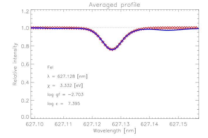
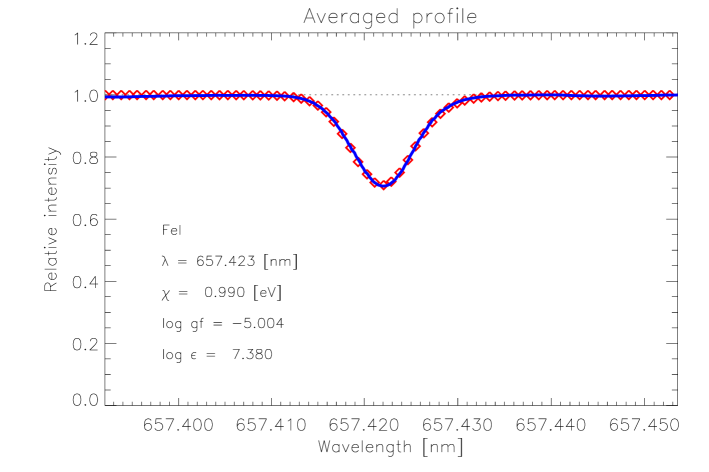
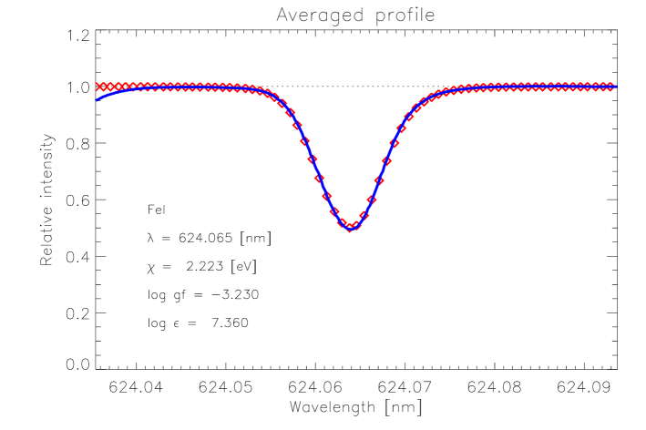
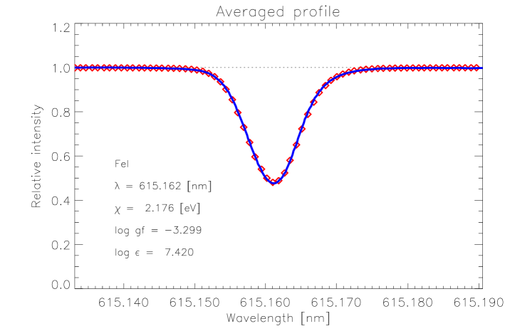
Figure 1: A few comparisons between the predicted (diamonds) and observed (solid lines) spatially and temporally averaged Fe i lines at disk-center ($\mu=1.0$). Only every other point in the theoretical profiles are shown for clarity. To illustrate the vast improvement over classical 1D model atmospheres, in the case of the Fe i 615.2 nm line (lower right panel) the corresponding prediction with the Holweger-Müller (1974) model atmosphere (dashed line) when adopting a microturbulence of 0.845 km s^-1 and a Gaussian macroturbulence of 2.4 km (the radial-tangential macroturbulence broadening is of course not applicable for intensity spectra) is also shown. The Fe abundance for the 1D profile has been adjusted to return the same equivalent width as the 3D profile (${\rm log}\,\epsilon_{\rm FeI}=7.59$) and the macroturbulence was determined by having the same line depths in 1D and 3D. The lack of line shift and asymmetry for the theoretical 1D profile is clearly seen. Note that all profiles are shown on an absolute wavelength scale with no arbitrary wavelength shifts

The derived Fe abundances obtained from profile fitting of the observed weak and intermediate strong Fe i lines are listed in Table 1. We emphasize that the abundances have been derived without invoking any equivalent widths, microturbulence or macroturbulence, leaving the elemental abundance as the only free parameter which is determined by the line strength. The good agreement between predicted and observed profiles is illustrated in Fig. 1; additional examples can be found in Paper I. It is interesting to contrast the remarkable consonance achieved with 3D hydrodynamical model atmospheres with the results from classical 1D model atmospheres, with or without macroturbulence (cf. Fig. 2; Paper I; Anstee et al. 1997); the improvement is equally obvious and telling.

As shown in Fig. 2, the individual abundances show no significant dependence on wavelength or excitation potential. We note that the claimed anomalous lines with excitation potential of 2.2 eV (Blackwell et al. 1995a) no longer exist in our calculations. Furthermore, there is no need to fine-tune the temperature structure to remove existing trends with excitation potential as necessary with the Holweger-Müller (1974) model with which there is about 0.15 dex difference in abundances between low- and high-excitation Fe i lines (Grevesse & Sauval 1999). There is, however, a slight trend with line strength in the sense that the strongest lines ($W_{\lambda}\simeq 9$ pm) imply about 0.06 dex higher abundances than the weakest lines. The reason for this behaviour will be discussed further in Sect. 7, although it has a minor impact on the final abundance estimates, as illustrated below. It is noteworthy that the trend is more pronounced for the Blackwell et al. (1995a) sample than for the lines of Holweger et al. (1995), which may partly explain why different microturbulences were adopted in the two studies. In terms of a 1D analysis, the trend would correspond to an underestimated microturbulence of about 0.15 km s^-1, which emphasizes the relatively minor magnitude of this shortcoming.

The resulting (unweighted) mean abundances of the Oxford and Hannover-Kiel samples of weak and intermediate strong Fe i lines are ${\rm log}\,\epsilon_{\rm FeI}=7.46\pm 0.04$ and ${\rm log}\,\epsilon_{\rm FeI}=7.43\pm 0.05$, respectively, where the quoted uncertainty is the standard deviation (twice the standard deviation of the mean = 0.02). The difference between the two samples essentially reflects the 0.03 dex offset in the absolute scales. From the combined sample the estimate is ${\rm log}\,\epsilon_{\rm FeI}=7.44\pm 0.05$; it should be noted here that nine lines in common have entered twice into this result. For reasons outlined above, we consider the transition probabilities of Blackwell et al. (1995a) to be slightly superior. However, due to the slight trend with line strength our final (unweighted) Fe determination is still the mean of all lines:

$${\rm log}\,\epsilon_{\rm FeI}=7.44\pm 0.04.$$

It should be noted that due to the inclusion of two different scales for the oscillator strengths, the scatter is slightly increased. The final uncertainty is most likely dominated by systematic rather than statistical errors, in particular the transition probabilities. Furthermore, the neglect of NLTE effects and observational complications such as blends and continuum level placement, may introduce additional abundance errors which are of comparable size; unfortunately astronomy has not yet reached the era with 0.02 dex accuracy in absolute abundances, in particular not with classical 1D model atmospheres, even if it is occasionally claimed in the literature.

The presence of a trend in derived abundances with line strength have a minor influence on the mean Fe abundance. Restricting the analysis to lines with $W_{\lambda}\leq 5$ pm decreases the mean abundances with 0.03 and 0.01 dex for the Oxford and Hannover-Kiel samples, respectively, while leaving the scatter practically intact. The larger sensitivity for the former lines can be traced to their in general larger line strengths. This is likely also the reason for the slightly larger difference in mean abundances between the two compilations than accounted for by the two $gf$-scales. It should be noted, however, that the Oxford sample only contains seven lines with $W_{\lambda}\leq 5$ pm, which may skew the results somewhat; additional weak Fe i lines with high-precision furnace oscillator strengths similar to the published Oxford data would certainly be of great value.

Given the excellent agreement between the predicted line shapes and observed profiles illustrated in Fig. 2 and Paper I, very similar abundances to those presented in Table 1 would be derived if equivalent widths or line depths had been used instead of profile fitting. Due to the larger uncertainties introduced by the subjectivity of equivalent width measurements and departures from LTE in the line cores, such abundance diagnostics are significantly more inferior compared to profile fitting, provided of course that the model atmosphere is sufficiently realistic to accurately predict the line profiles (Asplund et al. 2000a). It is interesting to note though that adopting the published equivalent widths of Blackwell et al. (1995) would result in a 0.02 dex higher Fe i abundance while using the Holweger et al. (1995) values would result in a 0.03 dex lower abundance than those derived from profile fitting for the two samples of lines.

It should be borne in mind that the analysis presented here assumes LTE, whose validity may be questioned in particular for Fe i lines. Unfortunately no detailed 3D NLTE calculations exist for solar Fe lines, and it is therefore difficult to predict how the abundances in Table 1 would be altered if departures from LTE would be allowed. Some preliminary guidance may come from 1D NLTE calculations (e.g. Solanki & Steenbock 1988). The calculations by Shchukina (2000, private communication) predict an over-ionization of Fe i and thus that the derived 1D LTE abundances are slightly underestimated by $\la 0.1$ dex with the Holweger-Müller (1974) model. Simply adopting these 1D corrections to our 3D LTE results would result in ${\rm log}\,\epsilon_{\rm FeI}=7.50\pm 0.07$ for the combined sample of Oxford and Kiel lines. Furthermore, the trend with line strength would become more pronounced ($\simeq 0.13$ dex difference between the strongest and weakest lines). Additionally a minor trend with excitation potential ($\simeq 0.03$ dex difference between $\chi_{\rm exc}=0$ and 4.5 eV transitions with low-excitation lines returning higher abundances) would appear. However, we are very reluctant to adopt these results here since it is premature to extrapolate 1D predictions to the 3D case until 3D NLTE calculations for Fe exist. Because the departures from LTE depend sensitively on the adopted model atmosphere, the temperature inhomogeneities may both amplify or attenuate the 1D NLTE effects. Naturally such 3D calculations would be of great interest.

Figure 2: The derived Fe abundance from weak and intermediate-strong Fe i lines as functions of wavelength (Upper panel), excitation energy (Middle panel) of the lower level, and line strength (Lower panel). The lines from the Blackwell et al. (1995a) and Holweger et al. (1995) samples are marked with $\bullet$ and $\circ$, respectively. The dashed lines are linear least square fits to the data when including all lines

5 Abundance from strong Fe i lines

Strong lines have since long been considered less than ideal for the purposes of abundance determinations due to the poorly understood collisional broadening which normally requires additional enhancement factors over the classical Unsöld (1955) recipe. Recent progress in the quantum mechanical treatment of the broadening (Anstee & O’Mara 1991, 1995; Barklem & O’Mara 1997; Barklem et al. 1998) has, however, opened up the possibility to use the damping wings of strong lines, which are little sensitive to the non-thermal broadening affecting weaker lines, as a complement to analyses of weaker lines when deriving elemental abundances. Anstee et al. (1997) found an excellent agreement with the meteoritic abundance for the thus determined Fe abundance from strong Fe i lines and the Holweger-Müller (1974) model.

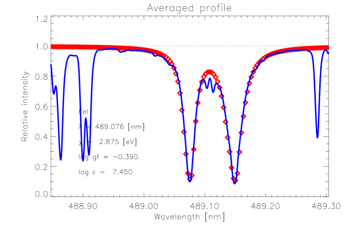
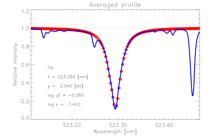
Figure 3: A few examples of the predicted (diamonds) and observed (solid lines) strong Fe i lines: Fe i 489.07+489.15 (Upper panel) and 523.9 nm (Lower panel) lines. Blending lines other than Fe lines have not been included in the synthesis

Table 2 lists the derived Fe abundances with our 3D hydrodynamical solar atmosphere model using a sample of strong Fe i lines which have been considered the most suitable by Anstee et al. (1997) (lines denoted by quality category A+, A and A- in their Table 1). Examples of the obtained agreement between predicted and observed profiles are found in Fig. 3. The resulting (weighted) mean Fe abundance from the 14 strong Fe i lines is

$${\rm log}\,\epsilon_{\rm FeI}=7.42\pm 0.03.$$

However, in spite of being considered as very accurate abundance diagnostics by Anstee et al. (1997), several of the lines turned out to unsuitable due to uncertainties introduced by severe blending, continuum placement, radiative broadening and poorly developed damping wings; those lines are marked in Table 2 and given half weight in the final abundance determination.

Even if the scatter is small for the sample of strong lines, it is noteworthy that the standard deviation ($\sigma=0.03$) is significantly larger than the claimed accuracy ($\sigma=0.01$) of the analysis by Anstee et al. (1997) using the Holweger-Müller (1974) model. In order to better understand the differences, we have therefore re-derived Fe abundances for the same lines in an identical procedure to that of Anstee et al. (1997), in particular using their collisional broadening data which differ slightly from those adopted in Table 2 which have been provided by Barklem (1999, private communication) from line-by-line calculations. Our results with the Holweger-Müller (1974) model have a significantly larger scatter than that quoted by Anstee et al. (1997), identical to our full 3D analysis of the same lines. We therefore suspect that the claimed uncertainty in Anstee et al. (1997) is over-optimistic and that the true scatter is larger, which is also verified by independent calculations by Barklem (1999, private communication). The choice of solar atlas (we adopt the more recent Brault & Neckel FTS-atlas while Anstee et al. use the older Liege atlas) has a minor influence on the resulting scatter, although strong lines are often conspicously asymmetric in the Liege-atlas (e.g. H$\alpha$), presumably due to inaccurate continuum tracement. Furthermore there is a systematic offset in theoretical line strengths which amounts to about 0.03 dex in abundance between our calculations and the identical ones by Anstee et al. (J. O’Mara, 1999, private communication). The reason for this discrepancy is likely due to slight differences in adopted continuum opacities, the $P_{\rm e}-P_{\rm gas}$-relation in the Holweger-Müller (1974) model and code implementation. This emphasizes again that derived abundances rarely have systematic errors smaller than 0.02 dex.

Due to the subjectivity involved with strong lines in terms of choice of solar atlas, continuum placement, wavelength shifts, blends, exactly which part of the wings are given the greatest weight, and remaining uncertainties in the collisional broadening, we consider abundances derived from strong lines to be inferior to those from weaker lines, although they naturally serve as important complements. In this respect it is reassuring that the here derived Fe abundance from strong Fe i lines agree well with those from weak and intermediate strong Fe i and Fe ii lines presented in Sects. 4 and 6.

6 Abundance from Fe ii lines

The Fe abundance values obtained from the individual Fe ii lines are listed in Table 3; a few examples of the achieved agreement between theory and observations are given in Fig. 4. As shown in Fig. 5, the individual abundances show no significant dependence on neither the wavelength, excitation potential of the lower level (though the adopted lines provide only a restricted range), nor the line strength. In this respect, the Fe ii lines differ from the Fe i lines, which show a minor trend with the line strength, at least within the assumption of LTE.

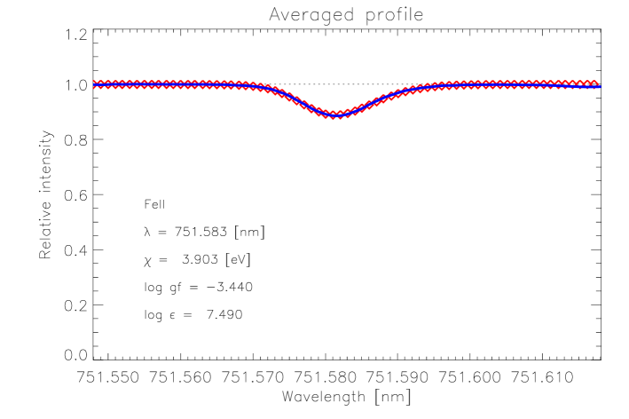
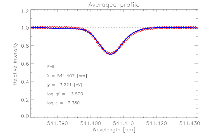
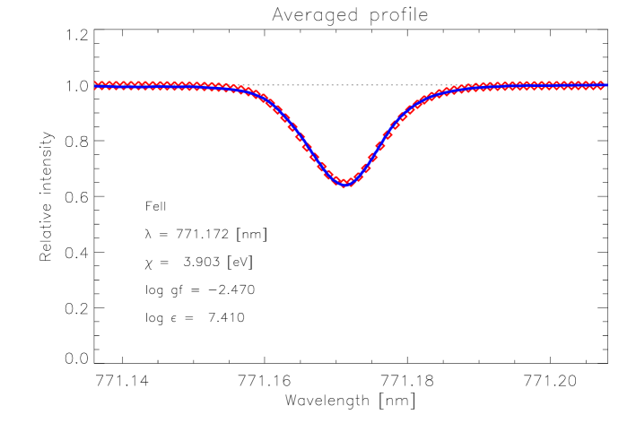
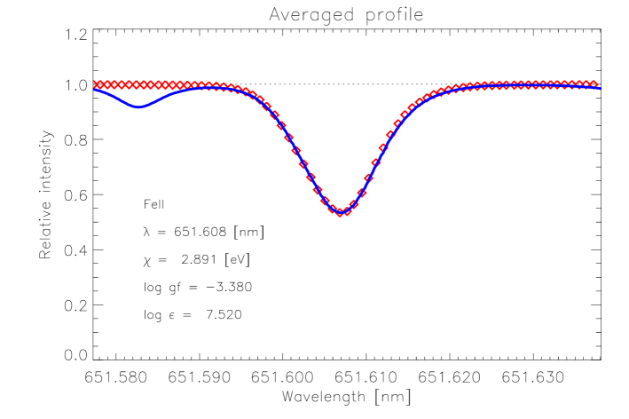
Figure 4: A few comparisons between the predicted (diamonds) and observed (solid lines) spatially and temporally averaged Fe ii lines at disk-center ($\mu=1.0$)

The resulting (unweighted) mean abundance becomes

$${\rm log}\,\epsilon_{\rm FeII}=7.45\pm 0.10,$$

where the quoted uncertainty is the standard deviation (twice the standard deviation of the mean = 0.05). The quoted error of course only reflects the internal accuracy and thereby possible uncertainties in e.g. the absolute scale of the $gf$-values are not accounted for. With Holweger et al.’s $gf$-values the mean abundance would be 0.04 dex higher while it would be 0.02 dex lower with the measurements given in Schnabel et al. (1999); the estimated error would remain basically unaltered by such exercises. As previously noted, with an Unsöld enhancement factor of 1.5 instead of 2.0 the abundance would be 0.01 dex higher. When excluding the discrepant Fe ii 744.93 nm line, which is significantly blended in the red wing, the mean abundance is increased by 0.01 dex; we also note that the $gf$-value for this line has a comparatively large uncertainty (Hannaford et al. 1992). Restricting to the ten lines with $W_{\lambda}<5.0$ pm, increases the mean abundance by only 0.006 dex, demonstrating that the observed trend with line strength only affects the Fe i lines.

The main advantage with Fe ii lines is their low sensitivity to details of the temperature structures and departures from LTE due to over-ionization. Furthermore, their weakness ensures that the lines are formed in the deeper layers which are less susceptible to NLTE excitation effects such as photon pumping and suction. The abundance derived from Fe ii lines should therefore be an accurate measure of the solar Fe abundance, provided the transition probabilities are reliable enough. It is reassuring that our average is in good agreement with the meteoritic value $7.50\pm 0.01$ (Grevesse & Sauval 1998), in particular in view of the uncertainty in the absolute $gf$-scales (Holweger et al. 1990; Hannaford et al. 1992; Schnabel et al. 1999) and that the meteoritic abundance scale probably needs to be adjusted downward by about 0.04 dex due to the revised photospheric Si abundance (Paper III).

7 Discussion

The results presented in Sects. 4, 5 and 6 paint a consistent picture for the solar photospheric Fe abundance. Both the weak Fe i and Fe ii lines suggest very similar abundances: ${\rm log}\,\epsilon_{\rm FeI}=7.44\pm 0.05$ and ${\rm log}\,\epsilon_{\rm Fe}=7.45\pm 0.10$. Since this result does not rely on equivalent widths, microturbulence, macroturbulence, or, at least for the Fe i lines, collisional damping enhancement factors, and is based on highly realistic 3D, hydrodynamical model atmospheres, it seems like the long-standing solar Fe problem (e.g. Blackwell et al. 1995a,b; Holweger et al. 1995) has finally been settled in favour of the meteoritic value, in particular considering the slight revision recently of the photospheric Si abundance and thus the whole absolute scale for the meteoritic abundances (Paper III): ${\rm log}\,\epsilon_{\rm Fe}=7.46\pm 0.01$. In fact the agreement between the photospheric and meteoritic values is partly fortuitious since the remaining uncertainties in oscillator strengths and model atmospheres are likely on the order of 0.04 dex.

The difference of 0.18 dex (7.64 vs 7.46) between our result and the one by Blackwell et al. (1995a) using the same set of $gf$-values is attributable to a switch to line profile fitting and improved collisional broadening treatment, and exchange of the microturbulence concept for self-consistent Doppler broadening from convective motions and the Holweger-Müller (1974) model for an ab initio 3D hydrodynamical model atmosphere. Our (unweighted) Fe ii result ${\rm log}\,\epsilon_{\rm FeII}=7.45\pm 0.05$ is similar to the (weighted) mean ${\rm log}\,\epsilon_{\rm FeII}=7.47\pm 0.04,$ found by Hannaford et al. (1991) using the same $gf$-values and the Holweger-Müller (1974) semi-empirical model atmosphere, which reflects the small sensitivity of the Fe ii lines to the details of the model atmospheres; indeed when instead of profile fitting the equivalent widths of Hannaford et al. (1991) are adopted the (unweighted) mean with the 3D solar model atmosphere is ${\rm log}\,\epsilon_{\rm FeII}=7.47\pm 0.04$. The main systematic error is no longer the model atmospheres and analysis as such, but is likely dominated by the accuracy of the transition probabilities, which still is on the level of 0.03 dex on average for both Fe i and Fe ii lines, even though the internal precision may be higher.

It is of interest to compare our findings for the solar Fe abundance with previously published studies based on 2D and 3D hydrodynamical models of the solar photosphere. Atroschenko & Gadun (1994) discuss derived Fe abundances from Fe i and Fe ii lines based on two different types of 3D model atmospheres (with $30^{3}$ and $32^{3}$ gridpoints, respectively, to compare with our simulation with the dimension 200 x 200 x 82) but obtain significantly more discrepant results than those presented here: ${\rm log}\,\epsilon_{\rm FeI}=7.05\pm 0.06$, ${\rm log}\,\epsilon_{\rm FeII}=7.48\pm 0.03$ and ${\rm log}\,\epsilon_{\rm FeI}=7.61\pm 0.02$, ${\rm log}\,\epsilon_{\rm FeII}=7.42\pm 0.02$, respectively; here the astrophysically determined $gf$-values for the Fe ii lines (using ${\rm log}\,\epsilon_{\rm Fe}=7.64$) have been rescaled to agree with the ones by Hannaford et al. (1992) which we have adopted. These results are, however, based on equivalent widths for selected lines and the use of microturbulence, which had to be introduced in an attempt to hide a very conspicious trend with equivalent width. Furthermore, the estimated abundances only made use of the very weakest lines and therefore represent underestimates for the Fe i lines. The discrepancies can likely be attributed to the use of gray opacities for the 3D model atmospheres and too small height extension, resolution and temporal sampling (the spectral synthesis was restricted to only one respectively two snapshots from the two simulation sequences and therefore should not be considered as proper temporal averages). These problems with not sufficiently realistic model atmospheres are also manifested in the relatively poor agreement with observed line profiles and asymmetries.

Figure 5: The derived Fe abundance from weak and intermediate-strong Fe ii lines as functions of wavelength (Upper panel), excitation energy of the lower level (Middle panel), and line strength (Lower panel). The dashed lines are linear least square fits to the data

The study of Gadun & Pavlenko (1997) suffer from similar problems. Their model atmospheres were 2D solar convection simulations (with 112 x 58 gridpoints) but properly temporally averaged. Utilizing equivalent widths, they derive ${\rm log}\,\epsilon_{\rm FeI}=7.33\pm 0.06$ and ${\rm log}\,\epsilon_{\rm FeII}=7.44\pm 0.02$ for their most reliable simulation sequence; again the Fe ii result have been rescaled for consistency with our analysis. Unfortunately, they do not show any comparison between predicted and observed line profiles, but judging from the differences in Fe abundances when derived from equivalent widths and line depths we conclude that the theoretical line profiles are too narrow, a common problem with a too poor numerical resolution in the simulations (Asplund et al. 2000a). To summarize, we are confident that our analysis is superior to previously published studies with multi-dimensional model atmospheres, a conclusion which is further supported by the excellent agreement between the predicted line profiles and asymmetries with observations, as described in detail in Paper I, and the confluence between the Fe i, Fe ii and meteoritic results (Paper III).

As noted in Sects. 4 and 6, neither the Fe i nor the Fe ii results depend on the wavelengths or the excitation potentials of the lines. Furthermore, the Fe ii lines show no trend with line strength, in spite of no microturbulence has entered the analysis, which, as explained in Paper I, is a consequence of the non-thermal Doppler broadening from the self-consistently calculated convective velocity field. However, according to Fig. 2 the individual Fe i abundances appear to depend slightly on the line strength, which could signal an underestimated rms vertical velocity in the line forming layers of the solar simulation (Paper I) or a too poor numerical resolution (Asplund et al. 2000a). But considering the good overall agreement for the theoretical and observed line shapes, which if anything suggests a slightly overestimated rms velocity (Paper I) and that no corresponding trend is present for the Fe ii (Fig. 5) and Si i (Paper III) lines, this conclusion seems less likely. Instead we suggest the existence of minor departures from LTE in the stronger lines, which causes the Fe abundances of these to be slightly overestimated. Such departures are more likely to affect Fe i than Fe ii lines and furthermore stronger lines are more susceptible than weak lines due to the decoupling of the non-local radiation field and local kinetic gas temperature in the higher atmospheric layers. Clearly an investigation of possible NLTE effects for Fe with 3D inhomogeneous model atmospheres would be interesting, similarly to the recent 3D calculations for Li (Kiselman 1997, 1998; Asplund & Carlsson 2000).

8 Conclusions

The application of ab initio 3D hydrodynamical model atmospheres of the solar photosphere to the line formation of Fe i and Fe ii lines has allowed an accurate determination of the solar photospheric Fe abundance. Since such a procedure does not invoke any free adjustable parameters besides the treatment of the numerical viscosity in the construction of the 3D, time-dependent, inhomogeneous model atmosphere and the elemental abundance in the 3D spectral synthesis, and considering that whole line profiles are fitted rather than equivalent widths, the results should provide a more secure abundance determination than previously accomplished. The confusion introduced by the various choices of mixing length parameters, microturbulence and macroturbulence no longer needs to cloud the conclusions. Furthermore, the analysis has made use of recent quantum mechanical calculations for the collisional broadening of the Fe i lines (Anstee & O’Mara 1991, 1995; Barklem & O’Mara 1997; Barklem et al. 1998), which removes the problematical damping enhancement parameters normally employed, at least for the Fe i lines. In view of these improvements, it is a significant accomplishment that a consistent picture is emerging in terms of Fe abundances: Fe i and Fe ii lines suggest ${\rm log}\,\epsilon_{\rm Fe}=7.44\pm 0.05$ and ${\rm log}\,\epsilon_{\rm Fe}=7.45\pm 0.10$, respectively, which agree very well with the meteoritic value ${\rm log}\,\epsilon_{\rm FeI}=7.46\pm 0.01$ (Paper III) given the remaining uncertainties in the transition probabilities. Fe sc i lines may be slightly more susceptible for departures from LTE but on the other hand the $gf$-values for Fe ii lines are somewhat less accurate. Our final best estimate for the photospheric Fe abundance is therefore simply the average of the two results, until detailed 3D NLTE calculations and improved measurements of the transition probabilities have been performed. Finally, the debate of the photospheric Fe abundance (e.g. Blackwell et al. 1995a,b; Holweger et al. 1995) seems to have been settled in favour of the low meteoritic abundance. Also strong Fe i lines imply a similar photospheric abundance: ${\rm log}\,\epsilon_{\rm FeI}=7.42\pm 0.03$ although we give this result lower weight due to the difficulties involved in analysing the wings of strong lines.

When comparing our results with other recent investigations of the solar Fe abundance, it is natural to ask why our study should be preferred. After all, traditional analyses using classical 1D model atmospheres, such as the Holweger-Müller (1974) model, has long been considered sufficient. However, as stricter demands are placed on the results in terms of accuracy, an improved analysis is required. Why should one embrace the results based on hydrostatic 1D model atmospheres, equivalent widths and ad-hoc broadening through microturbulence and macroturbulence, when such 1D models are inferior to the here presented ab initio 3D hydrodynamical models in terms of the observational diagnostics available for the Sun, such as granulation topology, velocities and statistics, time-scales and length-scales of the convection, continuum intensity brightness contrast, detailed spectral line profiles, asymmetries and shifts, flux distribution, limb-darkening and H-line profiles (e.g. Stein & Nordlund 1998; Asplund et al. 1999b; Paper I)? We leave it for the reader to ponder this rhetorical question.

- (1) Allende Prieto C., García López R.J., 1998a, A&AS 131, 431
- (2) Allende Prieto C., García López R.J., 1998b, A&AS 129, 41
- (3) Allende Prieto C., Ruiz Cobo B., García López R.J., 1998, ApJ 502, 951
- (4) Anstee S.D., O’Mara B.J., 1991, MNRAS 235, 549
- (5) Anstee S.D., O’Mara B.J., 1995, MNRAS 276, 859
- (6) Anstee S.D., O’Mara B.J., Ross J.E., 1997, MNRAS 284, 202
- (7) Asplund M., 2000, A&A, in press (Paper III)
- (8) Asplund M., Nordlund Å., Trampedach R., Stein R.F., 1999a, A&A 346, L17
- (9) Asplund M., Nordlund Å., Trampedach R., 1999b, in: Theory and tests of convection in stellar structure, ASP conf. series 173, A. Gimenez, E.F. Guinan and B. Montesinos (eds.), p. 221
- (10) Asplund M., Carlsson M., 2000, submitted to A&A
- (11) Asplund M., Ludwig H.-G., Nordlund Å., Stein R.F., 2000a, A&A, in press
- (12) Asplund M., Nordlund Å., Trampedach R., Allende Prieto C., Stein R.F., 2000b, A&A, in press (Paper I)
- (13) Atroshchenko I.N., Gadun A.S., 1994, A&A 291, 635
- (14) Barklem P.S., O’Mara B.J., 1997, MNRAS 290, 102
- (15) Barklem P.S., O’Mara B.J., Ross J.E., 1998, MNRAS 296, 1057
- (16) Barklem P.S., Piskunov N., O’Mara B.J., 2000, A&AS 142, 467
- (17) Basu S., 1998, MNRAS 298, 719
- (18) Bell R.A., Paltoglou G., Tripicco M.J., 1994, MNRAS 268, 771
- (19) Biémont E., Daudoux M., Kurucz R.L., et al., 1991, A&A 249, 539
- (20) Blackwell D.E., Lynas-Gray A.E., Smith G., 1995a, A&A 296, 217
- (21) Blackwell D.E., Smith G., Lynas-Gray A.E., 1995b, A&A 303, 575
- (22) Böhm-Vitense E., 1958, Z. Astroph. 46, 108
- (23) Brault J., Neckel H., 1987, Spectral atlas of solar absolute disk-averaged and disk-center intensity from 3290 to 12510 Å, available at ftp.hs.uni-hamburg.de/pub/outgoing/FTS-atlas
- (24) Canuto V.M., Mazzitelli I., 1991, ApJ 370, 295
- (25) Delbouille L., Neven L., Roland G., 1973, Photometric atlas of the solar spectrum from to , Liege
- (26) Freytag B., Ludwig H.-G., Steffen M., 1996, A&A 313, 497
- (27) Gadun A.S., Pavlenko Y.V., 1997, A&A 324, 281
- (28) Gray D.F., 1992, The observation and analysis of stellar photospheres, Cambridge University Press
- (29) Grevesse N., Sauval A.J., 1998, in: Solar composition and its evolution – from core to corona, Frölich C., Huber M.C.E., Solanki S.K., von Steiger R. (eds). Kluwer, Dordrecht, p. 161
- (30) Grevesse N., Sauval A.J., 1999, A&A 347, 348
- (31) Guo B., Ansbacher W., Pinnington E.H., Ji Q., Berends R.W., 1992, Phys. Rev. A 46, 641
- (32) Gustafsson B., Jørgensen U-G., 1994, A&AR 6, 19
- (33) Gustafsson B., Bell R.A., Eriksson K., Nordlund Å., 1975, ApJ 42, 407
- (34) Hannaford P., Lowe R.M., Grevesse N., Noels A., 1992, A&A 259, 301
- (35) Heise C., Kock M., 1990, A&A 230, 244
- (36) Holweger H., Müller E.A., 1974, Solar Physics 39, 19
- (37) Holweger H., Heise C., Kock M., 1990, A&A 232, 510
- (38) Holweger H., Kock M., Bard A., 1995, A&A 296, 233
- (39) Kim, Y-C., Chan, K.L., 1998, ApJ 496, L121
- (40) Kiselman D., 1997, ApJ 489, L107
- (41) Kiselman D., 1998, A&A 333, 732
- (42) Kostik R.I., Shchukina N.G., Rutten R.J., 1996, A&A 305, 325
- (43) Kupka F., Piskunov N.E., Ryabchikova T.A., et al., 1999, A&AS 138, 119
- (44) Kurucz R.L., 1993, CD-ROM, private communication
- (45) Lambert D.L., Heath J.E., Lemke M., Drake J., 1996, ApJS 103, 183
- (46) Ludwig H.-G., Freytag B., Steffen M., 1999, A&A 346, 111
- (47) Mihalas D., Däppen W., Hummer D.G., 1988, ApJ 331, 815
- (48) Milford P.N., O’Mara B.J., Ross J.E., 1994, A&A 292, 276
- (49) Nave G., Johansson S., Learner R.C.M., et al., 1994, ApJS 94, 221
- (50) Neckel H., 1999, Solar Physics 184, 421
- (51) Nissen P.E., Asplund M., Hill V., D’Odorico S., 2000, A&A, in press
- (52) Nordlund Å., 1982, A&A 107, 1
- (53) Nordlund Å., Dravins D., 1990, A&A 228, 155
- (54) O’Brian T.R., Wickliffe M.E., Lawler J.E., et al., 1991, J. Opt. Soc. Am. B8, 1185
- (55) Raassen A.J.J., Uylings P.H.M., 1998, A&A 340, 300
- (56) Rosenthal C.S., Christensen-Dalsgaard J., Nordlund Å., Stein R.F., Trampedach R., 1999, A&A 351, 689
- (57) Schnabel R., Kock M., Holweger H., 1999, A&A 342, 610
- (58) Solanki S.K., Steenbock W., 1988, A&A 189, 243
- (59) Stein R.F., Nordlund Å., 1989, ApJ 342, L95
- (60) Stein R.F., Nordlund Å., 1998, ApJ 499, 914
- (61) Trampedach R., Stein R.F., Christensen-Dalsgaard J., Nordlund Å., 1999, in: Theory and tests of convection in stellar structure, ASP conf. series 173, A. Gimenez, E.F. Guinan and B. Montesinos (eds.), p. 233
- (62) Unsöld A., 1955, Physik der Sternatmosphären, 2nd ed., Springer, Heidelberg