Line formation in solar granulation

Abstract

Realistic ab-initio 3D, radiative-hydrodynamical convection simulations of the solar granulation have been applied to Fe i and Fe ii line formation. In contrast to classical analyses based on hydrostatic 1D model atmospheres the procedure contains no adjustable free parameters but the treatment of the numerical viscosity in the construction of the 3D, time-dependent, inhomogeneous model atmosphere and the elemental abundance in the 3D spectral synthesis. However, the numerical viscosity is introduced purely for numerical stability purposes and is determined from standard hydrodynamical test cases with no adjustments allowed to improve the agreement with the observational constraints from the solar granulation.

The non-thermal line broadening is mainly provided by the Doppler shifts arising from the convective flows in the solar photosphere and the solar oscillations. The almost perfect agreement between the predicted temporally and spatially averaged line profiles for weak Fe lines with the observed profiles and the absence of trends in derived abundances with line strengths, seem to imply that the micro- and macroturbulence concepts are obsolete in these 3D analyses. Furthermore, the theoretical line asymmetries and shifts show a very satisfactory agreement with observations with an accuracy of typically $50-100$ m s^-1 on an absolute velocity scale. The remaining minor discrepancies point to how the convection simulations can be refined further.

1 Introduction

A proper understanding of convection has for a long time been one of the greatest challenges for stellar astrophysics. Since convection can strongly influence both the stellar evolution and the emergent stellar spectra, this uncertainty also carries over to other fields of astrophysics, such as galactic evolution and cosmology. Convection also plays a dominant role in various processes besides energy transport and stellar evolution, perhaps most notably mixing of nuclear-processed material, magnetic activity, chromospheric heating and stellar pulsations. Convection is furthermore of relevance in searches for extra-solar planets by introducing differential spectral line shifts that are likely to change periodically with solar-like cycles, and may then affect the measurements of periodic variations induced by orbiting companions.

The convection zone in late-type stars extends to the visible surface layers and thereby influences the emergent spectrum, from which virtually all information about the stars is deduced. For the Sun, the directly observable manifestation is granulation: an evolving pattern of brighter (warmer) rising material with darker (cooler) sinking gas in between, driven by the radiative cooling in a thin surface layer. Convection also leaves distinct signatures in the spectral lines in the form of line shifts and asymmetries (e.g. Gray 1980; Dravins et al. 1981; Dravins 1982; Dravins & Nordlund 1990a,b). For late-type stars, the bisectors of unblended lines have a characteristic $\subset$-shape, which results from the differences in line strength, continuum level, area coverage and Doppler shift between up- (granules) and downflows (intergranular lanes). Weak lines normally only show the upper part of the $\subset$-shape and have convective blueshifts (after removing the effects of the gravitational redshift). The cores of stronger lines are formed in or above the convective overshoot layers and therefore have smaller or non-existent blueshifts (Allende Prieto & García López 1998a,b). Solar transition region and coronal emission lines can, however, show significant redshifts of several km s^-1 (Doschek et al. 1976).

The possibility to obtain spectra of the Sun on an absolute wavelength scale (i.e. corrected for the radial velocity of the Sun relative to the spectrograph) with exceptionally high spectral resolution, signal-to-noise ratio (S/N) and wavelength coverage, makes the Sun an ideal testbench to study the physical conditions in the upper parts of the convection zone. For other stars one has previously been restricted to only a few spectral lines and poorer quality observations. Fortunately the situation has recently improved significantly (e.g. Allende Prieto et al. 1999, 2000), most notably concerning resolution, S/N and the use of carefully wavelength-calibrated spectra covering a large portion of the visual region.

In order to draw the correct conclusions from the observed stellar spectrum it is necessary to have a proper understanding of how convection modifies the atmospheric structure and the spectral line formation. Up to the present, theoretical models of stellar atmospheres have been based on several unrealistic assumptions, such as restriction to a 1-dimensional (1D) stratification in hydrostatic equilibrium with only a rudimentary parametrisation of convection through e.g. the mixing length theory (Böhm-Vitense 1958) or some close relative thereof (Canuto & Mazzitelli 1991). Such models therefore miss entirely the very nature of convection as an inhomogeneous, non-local and time-dependent phenomenon, which is driven by the radiative cooling at the surface. Furthermore, spectral synthesis using classical 1D model atmospheres show poor resemblance with observed spectra. In particular, the predicted line broadening is much too weak (of course, with no knowledge about the convective motions and Doppler shifts, all lines are also perfectly symmetric). To partly cure the problem, two artificial fudge parameters are introduced which the theoretical spectrum is convolved with to mimic the missing broadening: micro- and macroturbulence. In this situation, systematic errors arising from modeling inadequacies in e.g. chemical analyses of stars are far larger than the measuring errors alone. An improved theoretical foundation for the interpretation of stellar spectra is therefore highly desirable, to complement the impressive recent observational advances in terms of S/N, spectral resolution and limiting magnitudes following the new generation of large-aperture telescopes, like the ESO VLT and McDonald HET, and detectors.

With the advent of modern supercomputers, self-consistent 3D radiative hydrodynamical simulations of the surface convection in stars have now become tractable (e.g. Nordlund & Dravins 1990; Stein & Nordlund 1989, 1998; Asplund et al. 1999; Trampedach et al. 1999). These simulations invoke no free parameters like mixing length parameters except the numerical viscosity for stability purposes, yet succeed in reproducing key observational diagnostics such as granulation topology and statistics (Stein & Nordlund 1989, 1998), and helioseismic properties (Rosenthal et al. 1999). In the present paper we present a detailed study of the spectral line formation of Fe lines using such solar surface convection simulations as 3D model atmospheres. The resulting line shapes, shifts and asymmetries are found to compare very satisfactory with the observations, lending strong support to the realism of the simulations. The derived solar Fe abundances from weak and strong Fe i and Fe ii lines are presented in an accompanying article (Asplund et al. 2000b, hereafter Paper II). Subsequent papers in the series will deal with Si lines (Asplund 2000, hereafter Paper III) and observed and predicted spatially resolved solar lines (Kiselman & Asplund, in preparation, hereafter Paper IV). Additionally, hydrogen line formation will be the topic of a following article (Asplund et al., in preparation, hereafter Paper V).

2 Surface convection simulations

The 3D model atmospheres of the solar granulation which form the basis for the spectral line calculations presented here have been obtained with a 3D, time-dependent, compressible, radiative-hydrodynamics code developed to study solar and stellar surface convection (e.g. Nordlund & Stein 1990; Stein & Nordlund 1989, 1998; Asplund et al. 1999). The hydrodynamical equations of mass, momentum and energy conservation:

$$\frac{\partial{\rm ln}\rho}{\partial t}=-{\bf\bar{v}}\cdot\nabla{\rm ln}\rho-\nabla\cdot{\bf\bar{v}}$$ (1)

$$\frac{\partial{\bf\bar{v}}}{\partial t}=-{\bf\bar{v}}\cdot\nabla{\bf\bar{v}}+{\bf\bar{g}}-\frac{P}{\rho}\nabla{\rm ln}P+\frac{1}{\rho}\nabla\cdot\sigma$$ (2)

$$\frac{\partial e}{\partial t}=-{\bf\bar{v}}\cdot\nabla e-\frac{P}{\rho}\nabla\cdot{\bf\bar{v}}+Q_{\rm rad}+Q_{\rm visc}$$ (3)

coupled to the equation of radiative transfer along a ray (in total eight inclined rays):

$${\rm d}I_{\lambda}/{\rm d}\tau_{\lambda}=I_{\lambda}-S_{\lambda}$$ (4)

are solved on a non-staggered Eulerian mesh with 200 x 200 x 82 gridpoints; simulations with resolutions 100 x 100 x 82, 50 x 50 x 82 and 50 x 50 x 41 have also been computed but have not been utilized here since they are hampered by less good agreement between predicted and observed line profiles (Asplund et al. 2000a). In these equations, $\rho$ denotes the density, ${\bf\bar{v}}$ the velocity, ${\bf\bar{g}}$ the gravitational acceleration, $P$ the pressure, $e$ the internal energy, $\sigma$ the viscous stress tensor, $Q_{\rm visc}$ the viscous dissipation, $Q_{\rm rad}=\int_{\lambda}\int_{\Omega}\kappa_{\lambda}(I_{\lambda}-S_{\lambda}){\rm d}\Omega{\rm d}\lambda$ the radiative heating/cooling rate, $I_{\lambda}$ the monochromatic intensity, $S_{\lambda}=B_{\lambda}(T)$ the corresponding source function, $\tau_{\lambda}$ the optical depth and $\kappa_{\lambda}$ the absorption coefficient.

The physical dimension of the simulation box corresponds to 6.0 x 6.0 x 3.8 Mm of which about 1.0 Mm is located above continuum optical depth unity. Again, initial solar simulations extending only to heigths of 0.6 Mm suffered from problems in the predicted line asymmetries for strong lines which was traced to the influence of the outer boundary and that non-negligible optical depths were present in the line cores already at the outermost layers. Though not completely removed with the current more extended simulations, the problems have largely disappeared as discussed further in Sect. 6 and 7. The depth scale has been optimized to provide the best resolution where it is most needed, i.e. in those layers with the steepest gradients in terms of d$T$/dz and d${}^{2}T$/dz², which for the Sun occurs around the visible surface (which is defined to have a geometrical depth $z=0$ Mm). Through this procedure, sufficient depth coverage was also obtained in the important optically thin layers. The simulation box covers about 13 pressure scale heights and 11 density scale heights in depth, while the horizontal dimension is sufficient to include $\ga 10$ granules at any time of the simulation. The spatial derivatives are computed using third order splines and the time-integration is a third-order leapfrog predictor-corrector scheme (Hyman 1979; Nordlund & Stein 1990). The code was stabilized using a hyper-viscosity diffusion algorithm (Stein & Nordlund 1998) with the parameters determined from standard hydrodynamical test cases, like the shock tube. In this respect these parameters are not freely adjustable parameters for the surface convection simulations. It is important to realize that changing the numerical resolution in effect also varies the effective viscosity, which shows that the convective efficiency and temperature structure are independent on the adopted viscosity description (Asplund et al. 2000a). Periodic horizontal boundary conditions and open transmitting top and bottom boundaries were used in an identical fashion to the simulations described by Stein & Nordlund (1998). The influence of the boundary conditions on the results are negligible. In particular the upper boundary has been placed at sufficiently great heights not to disturb the line formation process except for the cores of very strong lines, and the lower boundary is located at large depths to ensure that the inflowing gas is isentropic and featureless. No magnetic fields or rotation were included in the present calculation.

In order to obtain a realistic atmospheric structure it is crucial to correctly describe the internal energy of the gas and the energy exchange between radiation and gas. For this purpose a state-of-the-art equation-of-state (Mihalas et al. 1988), which includes the effects of ionization, excitation and dissociation, has been used. Since the solar photosphere is located in the layers where the convective energy flux from the interior is transferred to radiation, a proper treatment of the 3D radiative transfer is necessary, which has been included under the assumption of LTE and using detailed continuous (Gustafsson et al. 1975 and subsequent updates) and line (Kurucz 1993) opacities. The 3D equation of radiative transfer was solved at each timestep of the convection simulation for eight inclined rays (2 $\mu$-angles and 4 $\varphi$-angles) using the opacity binning technique (Nordlund 1982). The four opacity bins correspond to continuum, weak lines, intermediate strong lines and strong lines; shorter tests with eight instead of four opacity bins revealed only very minor differences in the resulting atmospheric structures. The accuracy of the binning procedure was verified throughout the simulation at regular intervals by solving the full monochromatic radiative transfer (2748 wavelength points) in the 1.5D approximation (i.e. treating each vertical column separately in the flux calculations without considering the influence from neighboring columns) and found to always agree within 1% in emergent flux.

It is noteworthy that the convection simulations contain no adjustable free parameters besides those used to characterize the stars: the effective temperature $T_{\rm eff}$ (or equivalently, as adopted here, the entropy of the inflowing material at the bottom boundary), the surface acceleration of gravity log $g$ and the chemical composition. The entropy at the lower boundary was carefully adjusted prior to the simulation started in order to reproduce the total solar luminosity. The solar surface gravity (log $g=4.437$ [cgs]) was employed. The chemical composition of the gas were taken from Grevesse & Sauval (1998), in particular the Fe abundance used for the equation-of-state and opacity calculations was 7.50. The line opacities were interpolated to the adopted Fe abundance using the standard Kurucz ODFs with log$\,\epsilon_{\rm Fe}=7.67$ and non-standard ODFs computed with log$\,\epsilon_{\rm Fe}=7.51$ and without any He (Kurucz 1997, private communication, cf. Trampedach 1997 for details of the procedure).

3 Spectral line calculations and atomic data

From the full solar convection simulation, which covers two solar hours, a shorter sequence of 50 min with snapshots stored every 30 s was chosen for the subsequent spectral line calculations. The adopted snapshots have a temporally averaged effective temperature very close to the observed nominal $T_{\rm eff}=5777\pm 3\,$K for the Sun (Willson & Hudson 1988): $5767\pm 21$ K where the quoted range is the standard deviation of the individual snapshots. For our present purposes the time coverage is sufficient to obtain statistically significant spatially and temporally averaged line profiles and shifts, as verified by test calculations after dividing the snapshots in various sub-groups. Even as short sequences as 10 min produced line asymmetries and shifts to within 50 m s^-1 of the full calculations. In order to improve the vertical sampling, the simulation was interpolated to a finer depth scale with the same number of depth points but only extending down to layers with minimum continuum optical depths of $\tau_{\rm cont}=300$ ($\approx 700$ km below $\tau_{\rm cont}=1$ rather than $2.9\,$Mm in the original simulation). Prior to the line transfer computations, the snapshots were also interpolated to a coarser grid of 50 x 50 x 82 but with the same horizontal dimension to save computing time; various tests assured that the procedure did not introduce any differences in the spatially averaged line shapes or asymmetries. The Doppler shifts introduced by the convective motions in the 3D model atmosphere were correctly accounted for in the solution of the 3D spectral line transfer. In most cases, intensity profiles at the center of the solar disk ($\mu=1.0$) were considered, which have been calculated for every column of the interpolated snapshots, before spatial and temporal averaging and normalization. A few lines where, however, computed under different viewing angles to allow a disk-integration for comparison with published solar flux atlases (Kurucz et al. 1984). The assumption of LTE in the ionization and excitation balances and for the source function in the line transfer calculations ($S_{\nu}=B_{\nu}$) have been made throughout in the present study. The background continuous opacities were calculated using the Uppsala opacity package (Gustafsson et al. 1975 and subsequent updates).

Fe lines are the most natural tools to study line shapes and asymmetries in stars: Fe is an abundant element with a complex atomic structure which ensures there are many useful lines of the appropriate strength; there exists accurate laboratory measurements for the necessary atomic data such as transition probabilities and wavelengths (e.g. Blackwell et al. 1995; Nave et al. 1994); the Fe nuclei have a large atomic mass which minimizes the thermal velocities; the influence from isotope and hyperfine splitting should be negligible (e.g. Kurucz 1993); and LTE is a reasonable approximation for Fe (e.g. Shchukina & Trujillo Bueno 2000), at least for 1D model atmospheres of solar-type stars (3D NLTE studies of Fe may, however, reveal larger departures from NLTE as speculated by e.g. Nordlund 1985 and Kostik et al. 1996). By studying a large sample of neutral and ionized Fe lines with different atomic data and therefore line strengths, the solar photospheric convection at varying atmospheric layers can be probed by analysing the resulting line shifts and asymmetries. The Fe lines and their atomic data are the same as described in detail in Paper II. In particular, accurate laboratory wavelengths for the Fe i and Fe ii lines were taken from Nave et al. (1994) and Johansson (1998, private communication), respectively. The final profiles have been computed with the individual Fe abundances derived in Paper II.

For comparison with observations, the solar FTS disk-center intensity atlas by Brault & Neckel (1987) (see also Neckel 1999) has been used, due to its superior quality over the older Liege atlas by Delbouille et al. (1973) in terms of wavelength calibration (Allende Prieto & García López 1998a,b) and continuum tracement. For flux profiles the solar atlas by Kurucz et al. (1984) has been used, which is also based on FTS-spectra with a similar spectral resolution as the disk-center atlas. The wavelengths for the observed profiles have been adjusted to remove the effects of the solar gravitational redshift (633 m s^-1). All spatially averaged theoretical profiles have been convolved with an instrumental profile to account for the finite spectral resolution of the observed atlas. Since the atlas was acquired with a Fourier Transform Spectrograph (FTS), the instrumental profile corresponds to a sinc-function with $\lambda/\Delta\lambda\simeq 520\,000$ in the visual rather than the normal Gaussian (e.g. Gray 1992). The additional instrumental broadening has only a minor (but not entirely negligible) effect on the resulting line asymmetries due to the high resolving power of the FTS.

4 General features of 3D line formation

The convective motions and the atmospheric inhomogeneities leave distinct fingerprints in the spectral lines, which can be used to decipher the conditions in the line-forming layers produced by the convection (e.g. Dravins et al. 1981; Dravins & Nordlund 1990a,b). Line strengths of weak lines are predominantly determined by the average atmospheric temperature structure, while the line widths reflect the amplitude of the Doppler shifts introduced by the velocity fields. Line shifts and bisectors are created by the correlations between temperature and velocity and the details of the convective overshooting, as well as the statistical distribution between up- and downflows. Therefore, obtaining a good agreement between observed and predicted profiles lend strong support to the realism of the simulations.

4.1 Spatially resolved profiles

Figure 1: Spatially resolved profiles and bisectors for the Fe i 608.2 line. The lines are both stronger and have higher continuum intensities in the blueshifted granules compared with the red-shifted intergranular lanes. The largest vertical velocities in the photosphere are encountered in the downflows. The intensity scale is normalized to the spatially averaged continuum level. The thick solid lines correspond to the spatially averaged profile and bisector

Although Paper IV and V in the present series of articles will discuss in detail observed and predicted spatially resolved lines, a brief excursion is still warranted here in order to interpret the spatially averaged profiles and bisectors presented in Sects. 5, 6 and 7.

Spatially resolved profiles take on an astonishing range of shapes and shifts spanning several km s^-1, as illustrated in Fig. 1. The intensity contrast reversal in the higher layers of the photosphere, i.e. granules become dark while intergranular lanes become bright a few hundred km above the visible surface, is clearly seen in the cores of the resolved profiles. The strengths of spatially averaged profiles are normally biased towards the granules, since the upflows in general are brighter (high continuum intensity), have steeper temperature gradients and have a larger area coverage than the downflows. These trends are also observationally confirmed, which suggests that the combination of 3D hydrodynamical model atmospheres and LTE is appropriate for most Fe lines (Kiselman 1998; Kiselman & Asplund 2000; Paper IV).

Spatially resolved bisectors are not at all typical of the spatially averaged bisectors, which are merely the result of the statistical distribution of individual profiles. Rather than the characteristic $\subset$-shape bisectors, individual bisectors normally have inverted $\backslash$-shape bisectors in granules and $/$-shapes in intergranular lanes, as seen in Fig. 1. This reflects the in general increasing vertical velocities with depth in the photosphere. However, due to the meandering motion of the downflows, occasionally the line-of-sight passes through both upward and downward moving material which causes large variations for certain columns.

4.2 Spatially averaged disk-center profiles

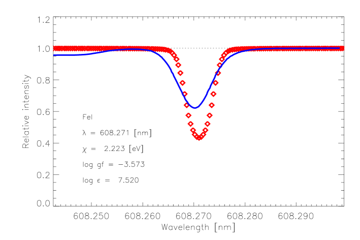
Figure 2: The spatially and temporally averaged Fe i 608.2 line when artificially removing all convective velocities in the simulations (diamonds). In comparison with the solar intensity atlas (solid line, Brault & Neckel 1987) the predicted line is much too narrow and lacks the correct line shift and asymmetry. The result when including the self-consistent velocity field is shown in Fig. 8

Figure 3: The spatially and temporally averaged Fe i 608.2 bisector assuming three different abundances: log $\epsilon_{\rm Fe}=7.00$, 7.50 and 8.00 (or equivalently with three different log $gf$-values). Note that the upper parts of the bisectors do not coincide for the different line strengths since the whole region of line formation is shifted outwards for stronger lines

Figure 4: The bisectors of the Fe i 608.2 (weak) and 621.9 nm (strong) lines (solid lines) which both have $\chi_{\rm exc}=2.2\,$eV. Also shown are the corresponding (artificial) Fe i lines with $\chi=1.2\,$eV (dotted lines) and $\chi=3.2\,$eV (dashed lines). The fake lines have all other transition properties the same as the original lines but with the $gf$-values ($\simeq\pm 1.0\,$dex) adjusted to return the same line depths. All lines have here been computed for the same 5 min sequence from the full convection simulation, which means that the bisectors differ slightly from the average of the whole 50 min simulation

Figure 5: The bisectors of the Fe i 608.2 (weak) and 621.9 nm (strong) lines (solid lines). Also shown are the corresponding (artificial) Fe i lines with $\lambda=500$ nm (dotted lines) and $\lambda=700$ nm (dashed lines). The fake lines have all other transition properties the same as the original lines but with the $gf$-values adjusted to return the same line depths. All lines have here been computed for the same 5 min sequence as in Fig. 4

The widths of spatially averaged spectral lines, which clearly exceed the natural and thermal broadening, predominantly arise from the velocity amplitude of the granules and intergranular lanes and to a lesser extent from photospheric oscillations. A demonstration of the importance of the non-thermal Doppler broadening is presented in Fig. 2, which shows the resulting spatially averaged profile from the 3D simulations but with all convective velocities artificially set equal to zero in the line calculation; thereby the predicted profile closely resemble those calculated with classical 1D model atmospheres. Clearly, without the Doppler shifts the line is much too narrow, which requires additional broadening in the form of micro- and macroturbulence to be introduced. The poor agreement between observations and predictions when not including the self-consistent velocity field as shown in Fig. 2, should be contrasted with the excellent fit shown in Fig. 8.

The individual line bisectors depends on the details of the line formation and thus on transition properties such as log $gf$, $\chi_{\rm exc}$ and $\lambda$ in an intricate way, as illustrated in Fig. 3, 4 and 5. When discussing mean bisectors (e.g. Gray 1992; Allende Prieto et al. 1999; Hamilton & Lester 1999) it is therefore important to consider only appropriate subgroups consisting of lines with similar characteristics to avoid introducing errors when interpreting the results in terms of convective properties. As a corollary, it follows that reconstructing a mean bisector by averaging bisectors or using shifts of lines of different strengths will in general not recover in detail the individual bisectors, as exemplified in Fig. 3. As expected, for line depths $\ga 0.5$ the bisectors closely coincide for lines of different strengths due to the disappearance of the influence from the convective inhomogeneities. Similarly, decreasing the excitation potential tends to shift the line formation outwards, producing less convective blueshifts for a given line depth (Fig. 4), while decreasing the wavelength increases the brightness contrast and makes the temperature gradients steeper, resulting in more vigorous convective line asymmetries (Fig. 5).

Figure 6: The temporal evolution of the spatially averaged profile and bisector for the Fe i 608.2 line. The 40 profiles shown here are taken at one minute intervals from the full solar simulation. The intensity scale is normalized to the averaged continuum level for the full simulation sequence

The temporal evolution of the granulation pattern also introduce changes in the line profiles. Solar granules have typical lifetimes of about 10 min but since the numerical box covers typically $\ga 10$ granules at any time, the influence of growing and decaying granules are relatively modest, as illustrated in Fig. 6. Since the emergent $T_{\rm eff}$ is not enforced but rather is the result of the evolving granulation pattern, the continuum level varies slightly ($\approx\pm 2\%$, corresponding to $T_{\rm eff,rms}=20\,$K) throughout the simulation, as well as the line strength. The bisector shapes are only slightly modified by the granulation, though the presence of oscillations in the simulation box shifts the bisectors back and forth in a regular fashion with a period corresponding to the solar 5 min oscillations. These numerical oscillations have an amplitude of about $\pm 300$ m s^-1 in the line-forming layers. The oscillations additionally broaden the line, though without altering the line strength since essentially the whole photosphere oscillates in unison without modifying the atmospheric structure.

4.3 Spatially averaged off-center intensity and disk-integrated flux profiles

Although not the main emphasis of the present paper a few Fe lines have been computed at different viewing angles (4 $\mu$-angles and 4 $\varphi$-angles) in order to enable a disk-integration to obtain flux profiles. A disk-integration requires further that the rotational broadening (1.8 km s^-1 in the case of the Sun) is taken into account. The line formation of flux profiles is more complex than for intensity profiles due to the contributions from different disk positions. The well-known limb-darkening decreases the continuum intensities towards the limb but the lines also tend to be weaker due to the more shallow temperature gradient in the upper atmosphere. Furthermore, the granulation contrast decreases towards the limb, since higher layers with progressively smaller influence of the granulation is seen. At a given instant the line asymmetries vary significantly more towards the limb as the line-of-sight may pass through both granules and intergranular lanes and also the horizontal velocities may introduce Doppler shifts. Thus the Doppler shifts are less well correlated with the background continuum intensity, which introduces a more random nature of the resulting bisectors for inclined line-of-sights.

Figure 7: The spatially and temporally averaged Fe i 608.2 profile and bisector at different viewing angles. The line has been computed at 4 $\mu$-angles and 4 $\varphi$-angles. The profiles have been normalized to the continuum intensity at disk center. The thick solid lines represent the profile and bisector of the line at disk-center. Note the ”limb effect” in the bisectors: smaller convective blue-shift toward the limb

Fig. 7 illustrates the variation of the spatially and temporally averaged intensity profiles and bisectors of a weak Fe i line at various viewing angles, which make up the necessary profiles for a disk-integration. Also seen is the limb-effect (Halm 1907): the wavelength of solar lines increases towards the limb such that at small $\mu$ the typical convective blueshift seen at disk-center has disappeared completely or even been reversed into a small red-shift when removing the effects of gravitational redshift and rotation. The limb-effect is the same effect as present between strong and weak lines, namely that the core of the lines are formed in high enough photospheric layers where the granulation contrast and velocities have largely vanished. The red-shifted cores at very small $\mu$, which are both observed and predicted with the 3D model atmospheres, are likely due to a bias for receding horizontal velocities to be viewed against the higher temperatures above intergranular lanes while the approaching gas will preferentially be seen against the lower temperatures above granules due to the temperature reversal in the higher photospheric layers (Balthasar 1985).

5 Solar Fe line shapes

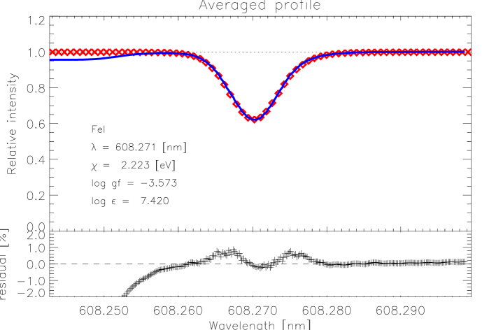
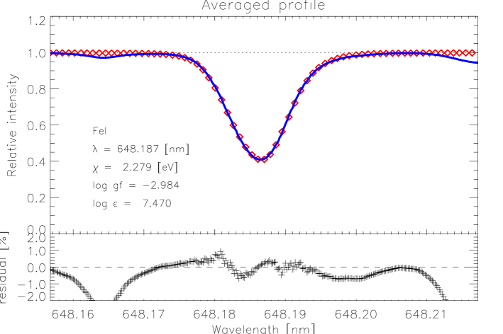
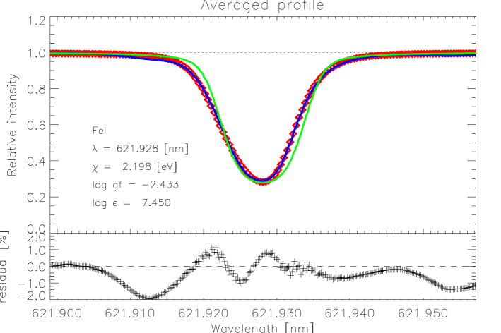
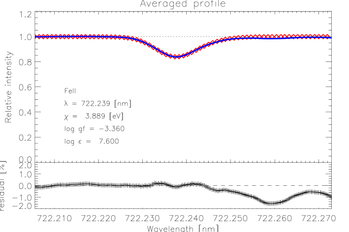
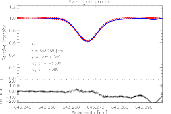
Figure 8: Some examples of spatially and temporally averaged disk-center Fe i and Fe ii lines (diamonds) compared with the observed solar atlas (solid lines, Brault & Neckel 1987). Also shown are the residual intensities (observed - predicted) to emphasize the remaining minor differences; minor blends not included in the spectral synthesis are clearly seen in some of the line wings. The predicted profiles have been convolved with a sinc-function to account for the finite spectral resolution of the solar atlas. Minor corrections to the observed wavelengths ($<100$ m s^-1) and continuum level ($<1\%$) have been allowed to improve the fits. The Fe lines are almost perfectly matched by the theoretical profiles, which implies that the rms velocity amplitudes in the simulations are very close to the real values in the solar photosphere. For comparison the best fit 1D profile for the Fe i 621.9 nm line is also shown (green solid line in the middle right panel), which has been computed with the Holweger-Müller (1974) model atmosphere, log$\,\epsilon_{\rm FeI}=7.60$ (to achieve the same equivalent width as the 3D profile), $\xi_{\rm turb}=0.845$ km s^-1 and convolved with a Gaussian macroturbulence of 1.6 km s^-1 to have the correct line depth (radial-tangential macroturbulence is not applicable for intensity profiles, Gray 1992); clearly the agreement is much inferior in spite of the adjustable broadening parameters due to the neglect of convective velocities and spatial inhomogeneities

The Doppler shifts introduced by the convective flow velocities in the photosphere cause significant line broadening beyond the thermal, radiative and collisional broadening. Fig. 8 shows a few examples of spatially and temporally averaged Fe i and Fe ii lines at disk-center calculated using the 3D solar simulation together with the corresponding observed intensity profiles; additional examples are given in Paper II. Clearly the agreement is very satisfactory for unblended Fe i and Fe ii lines with almost a perfect match. In contrast, theoretical 1D profiles are clearly discrepant in spite of the presence of both a micro- and macroturbulence (as exemplified by the Fe i 621.9 nm line which is shown in the middle panel of Fig. 8). The residual intensities amount to only $<1\%$, which is accomplished without any micro- or macroturbulent broadening. The FWHM of the Fe lines typically agree to within 1%. Fig. 9 shows the disk-integrated flux profiles of two Fe i lines as compared with the solar flux atlas of Kurucz et al. (1984) and again the agreement is very encouraging. In fact, given the good agreement in general for both intensity and flux profiles, blending lines, which may otherwise have gone undetected in a 1D analysis, are easily identified.

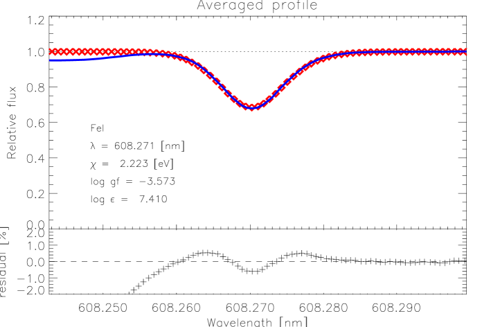
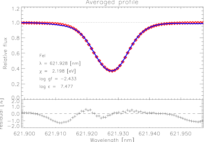
Figure 9: The predicted flux profiles of the Fe i 608.2 and 621.9 nm lines (diamonds) compared with the solar flux atlas (solid lines, Kurucz et al. 1984). The theoretical lines have been disk-integrated using a solar rotational velocity of $v_{\rm rot}{\rm sin}i=1.8$ km s^-1 and convolved with sinc-function to account for the finite spectral resolution of the FTS-atlas

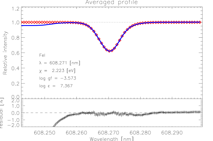
Figure 10: The predicted spatially and temporally averaged profile of the Fe i 608.2 line (diamonds) using a solar simulation based on a previous equation-of-state and line opacities (Gustafsson et al. 1975 with subsequent updates instead of Mihalas et al. 1988 and Kurucz 1993) compared with the solar disk-center intensity atlas (solid lines, Brault & Neckel 1987). The agreement is even better than the corresponding profile shown in Fig. 8

Although the overall agreement is very satisfactory, it is clear from a closer inspection of Figs. 8 and 9 that there are systematic discrepancies in the line profiles which are appearent in most intensity and flux profiles, in particular the weaker lines. The cores of the predicted lines tend to be slightly too shallow while the near line wings are somewhat too broad, which suggests a slightly over-estimated rms vertical velocity amplitude in the solar simulation. The slightly problematic line cores may also signal departures from LTE (cf. Rutten & Kostik 1982), which is more likely to affect the cores than the wings. Furthermore, the cores of intermediate strong lines tend to be displaced compared with observations; the latter feature will be discussed further in Sects. 6 and 7. It should not come as a surprise that the cores of the stronger lines show discrepancies, since the highest atmospheric layers are likely the least realistic due to still missing ingredients in the simulations and spectral synthesis in terms of e.g. departures from LTE and the inexact line blanketing treatment in the actual convection simulation.

The minor disagreements shown by the Fe lines are very important, since they point to how the simulations can be improved further. Prior to the convection simulations used here, we have carried out several similar solar simulations which differed from the present ones, most notably in terms of equation-of-state and opacities (Gustafsson et al. 1975 with subsequent updates vs. Mihalas et al. 1988 and Kurucz 1993), height extension ($z_{\rm min}=-0.6$ vs. $-1.0$ Mm) and numerical resolution (100 x 100 x 82, 50 x 50 x 82 and 50 x 50 x 63 vs. 200 x 200 x 82). In all cases they suffered from more pronounced problems in terms of line asymmetries, which were subsequently addressed with the more refined and improved simulations. However, it is noteworthy that the overall shapes of weak Fe lines illustrated in Figs. 8 and 9 were even better described with the previous equation-of-state and line opacities (Gustafsson et al. 1975 with subsequent updates), as seen Fig. 10, although with a slightly smaller Fe abundance. One may speculate that the older equation-of-state better describes the conditions typical of the line-forming layers than the more recent version (Mihalas et al. 1988) which has been optimized for stellar interiors. But it may also be coincidental, since the differences in line profiles are relatively small and there are also additional differences in terms of resolution (253 x 253 x 163) and $z_{\rm min}$ ($-0.6$ Mm) between the two simulations. A further investigation into the matter would, however, be interesting.

6 Solar Fe line shifts

Figure 11: Upper panel: The predicted (open circles) and observed (stars) line shifts for Fe i lines as a function of equivalent widths. The equivalent widths are taken from Blackwell et al. (1995), Holweger et al. (1995) and Moore et al. (1966), in this order of preference. Lower panel: The differences between predicted and observed line shifts. The gravitational red-shift of 633 m s^-1 has been subtracted from the observed line shifts. The agreement is very good for weak and intermediate strong lines but becomes progressively worse for stronger lines. Most of the scatter for the weaker lines is probably due to uncertainties in laboratory wavelengths and blends

Figure 12: Same as Fig. 11 but for the 15 Fe ii lines. The equivalent widths are taken from Hannaford et al. (1992)

Figure 13: Same as Fig. 11 but as a function of excitation potential of the lower level. In general high excitation lines are formed in deeper layers and thus have larger convective blueshifts. The trend is not as striking as in Fig. 11, since also e.g. the oscillator strength determines the line-formation depth

A major advantage with solar observations compared with corresponding stellar observations is the existence of high-quality spectral atlases given on an absolute velocity scale, which is possible since the differential radial velocity between the Sun and the Earth can be accurately corrected for (e.g. Kurucz et al. 1984; Brault & Neckel 1987; Neckel 1999). Furthermore, the well-determined solar mass and radius allow the solar gravitational redshift of 636 m s^-1, or 633 m s^-1 for light intercepted on Earth (Lindegren et al. 1999), to be estimated, leaving the remaining shifts to be attributed to convection as pressure shifts and similar line shifts are of much lesser importance (e.g. Allende Prieto 1998). Solar spectral lines show different line shifts depending on the typical depths of formation of the line cores. Unfortunately, the remaining uncertainties in the individual laboratory wavelengths and possible blends cause a scatter of about 100 m s^-1 in the observed line shifts, in particular for the weaker lines.

Through the self-consistently calculated convective flows in the solar simulations the predicted line shifts can be directly compared with observations on an absolute wavelength scale. Figs. 11 and 12 show the calculated line shifts for Fe i and Fe ii lines, respectively; we prefer to plot the shifts vs line strengths rather than vs line depths as Hamilton & Lester (1999), since due to saturation the latter method will not detect clearly the gravitional redshift plateau (Allende Prieto & García López 1998a). Weaker lines show as expected more prominent blueshifts and Fe ii lines more so than Fe i lines due to their in general deeper layers of formation. The maximum predicted blueshift for Fe i lines is 550 m s^-1 while it reaches 800 m s^-1 for Fe ii lines. A trend between line shift and excitation potential is present (Fig. 13) but much less pronounced due to the obscuration introduced by the $W_{\lambda}$- and $\lambda$-dependencies (cf. Fig. 3, 5 and Hamilton & Lester 1999).

As clear from Figs. 11 and 12 the predicted line shifts agree well with observations for weak and intermediate strong lines. The average difference for weak ($W_{\lambda}\la 6\,$pm) Fe i lines is $0\pm 53$ m s^-1 ($0.000\pm 0.053$ km s^-1), while when including also the intermediate strong lines ($W_{\lambda}\la 10\,$pm) the corresponding difference increases to $51\pm 81$ m s^-1; in these estimates we have not included the Fe i 666.8 nm line ($W_{\lambda}=0.89\,$pm) as we suspect that it has an erroneous laboratory wavelength, since it is significantly more discrepant (300 m s^-1) than other lines with similar strengths. The situation is slightly worse for the Fe ii lines with a mean difference of $-64\pm 85$ m s^-1 for all 15 lines with $W_{\lambda}\la 10\,$pm. However, the laboratory wavelengths for Fe ii lines are likely of somewhat poorer quality than the Fe ii lines and there are unfortunately only few available lines of the appropriate strengths.

Figure 14: The time averaged horizontal average (solid) and rms (dashed) vertical velocity in the solar simulations. Positive vertical velocities indicate downward motion. Note the upturn in $\langle v_{\rm z}\rangle$ which reaches 400 m s^-1 in the uppermost parts of the atmosphere. The horizontal part of the curves at the upper boundary is a consequence of the boundary formulation, which specifies the same vertical velocity in the two top layers

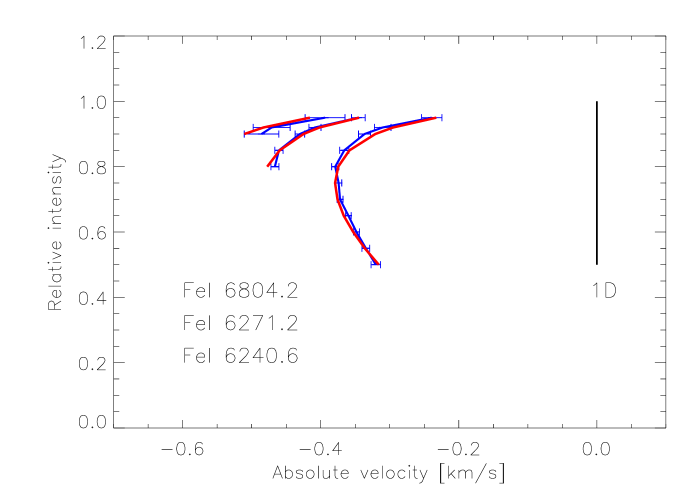
Figure 15: The predicted (solid line) and observed (line with error bars) bisectors of the Fe i 680.4, 627.1 and 624.0 nm (in order of increasing line strength) lines. It should be emphasized that the velocity scale is absolute for both the computed and measured line asymmetries, i.e. no arbitrary wavelength shifts have been applied in order to bring the two into agreement. Clearly the predicted bisectors agree rather satisfactory with the observations. In fact, the close resemblance for these lines is partly fortuitous since both the laboratory wavelengths and the wavelength calibration of the solar intensity atlas may only be accurate to about $30-50$ m s^-1. In comparison, classical 1D model atmospheres will of course only produce vertical bisectors at zero absolute velocity

As evident from Figs. 11 and 12, the correspondance between predictions and observations becomes progressively worse for stronger Fe i and Fe ii lines; a trend with $W_{\lambda}$ in the line shift differences may also extend to weaker Fe ii lines, according to Fig. 12. We attribute this effect predominantly to the influence of the outer boundary in the spectral line calculations but departures from LTE may also play a role. The cores of these strong lines have significant optical depths already at the uppermost depth layers where the average vertical velocity is directed downwards, as shown in Fig. 14. This follows from having on average no net mass flux, since the downward moving material in general has smaller densities and thus larger velocities in these layers. Since the temperature-velocity correlations present further in has essentially completely disappeared at these large heights, this results in convective redshifts, which do not seem to be present in the observational evidence (Allende Prieto & García López 1998a). The discrepancy was noticably larger in the simulations with smaller extension (maximum height of 0.6 Mm) and numerical resolution (Asplund et al. 2000a). We therefore consider the effect as a numerical artifact, which should be possible to further reduce by using an improved treatment of the outer boundary and higher numerical resolution. In spite of the remaining shortcomings, differential line shifts are very accurate; the main uncertainty is of observational (blends and laboratory rest wavelengths) nature.

7 Solar Fe line asymmetries

Line asymmetries carry additional information to line shifts, since the lines trace the atmospheric structure throughout the line forming region and not only the higher layers where the core is formed and thus the line shift. Fig. 15 shows a few examples of the predicted line asymmetries and the corresponding observed bisectors. It should be noted that both types of bisectors are on an absolute wavelength scale and the synthetic bisectors have therefore not been shifted in velocity to match the observations. In order to achieve such a remarkable agreement it is necessary to have both a very accurate description of the atmospheric structure and the details of line formation as well as very high quality laboratory wavelengths. Clearly the result is very satisfactory. The excellent correspondance in Fig. 15 is not only fortuitous, as is apparent from an inspection of Fig. 16, which shows the differences in observed and predicted line asymmetries for all the 67 computed Fe i lines. Under ideal conditions the differences should all be vertical lines with no velocity offset, which in fact is not far from the truth. In particular the weaker lines show excellent agreement, while the situation becomes progressively worse for the cores of the stronger lines, reflecting the shortcomings already discussed in Sect. 6. This discrepancy also affects the bisectors closer to the continuum for the stronger lines, causing the bisector differences to be predominantly positive. The situation for the Fe ii lines are shown in Fig. 17, which again is very satisfactory. Both with an inferior resolution and height extension in the convection simulations the resulting bisectors are of noticably lower quality when comparing with observations (Asplund et al. 2000a). The good overall agreement in terms of line asymmetries therefore lend very strong support to the realism of the convection simulations.

Figure 16: Differences between predicted and observed bisectors for the Fe i lines used for the present analysis; a gravitational red-shift of 633 m s^-1 has been subtracted for the observed bisectors. Except for a tendency for the predicted strong lines (line depths greater than 0.5) to have slightly too little blueshift or too much redshift, as also obvious in Fig. 11, the agreement is clearly very satisfactory. The line furthest to the left is Fe i 666.8 nm, whose laboratory wavelength therefore can be suspected to be slightly in error

Figure 17: Same as Fig. 16 but for the 15 Fe ii lines

In fact it is very easy to detect problematic lines due to erroneous laboratory wavelengths (large velocity offset) and blends (discrepant bisector shape) when comparing line asymmetries. It can be mentioned that initially the wavelengths for the Fe i 697.2 and 718.9 nm lines were accidentally taken from the VALD database rather than from Nave et al. (1994), which differed by only 16 and 5 mÅ (corresponding to 0.7 and 0.2 km s^-1), respectively, though immediately detected when analysing the line asymmetries. Furthermore, the Fe ii wavelengths provided by Johansson (1998, private communication) were found to be of significantly higher quality than the ones given in Hannaford et al. (1992).

8 The nature of macro- and microturbulence

The concepts of micro- and macroturbulence are introduced in 1D analyses in order to account for the missing line broadening on length scales less than and larger than a unit optical depth, respectively. Naturally such a simplistic division is artificial since the motions occur on a range of scales. Furthermore, they are supposed to represent turbulent motions and thus are normally assumed to be isotropic. In reality the appearance of the photospheric granular velocities is clearly more laminar than turbulent with distinct upflows and downflows, a direct consequence of the strong density stratification (Nordlund et al. 1997). Given the evidences presented here and in Papers II and III, there appears to be no need to invoke any macro- or microturbulence in spectral syntheses based on realistic 3D model atmospheres.

The excellent agreement between predicted and observed line profiles shown in Fig. 8 implies that the theoretical lines have the correct widths without the use of any macroturbulence. The classical concept of macroturbulence can therefore be fully explained by the self-consistently calculated convective velocity fields and the stellar oscillations. It is less obvious that the simulations properly account for the small-scale motions normally referred to as microturbulence given the finite numerical resolution which may or may not resolve all significant velocities. We believe, however, that the currently best solar simulations described here are of sufficiently high resolution to describe also the most important effects of these small-scale motions. Firstly, solar simulations with different numerical grid resolutions indicate that the velocity distributions have essentially converged already at a resolution of 200 x 200 x 82, which is also apparent from the predicted line shapes (Asplund et al. 2000a). The contribution from unresolved scales should therefore be very minor. We emphasize that a high resolution is needed in the construction of the 3D model atmospheres to allow the high-velocity tails of the velocity distributions, but that smaller resolutions can be used for the spectral synthesis, as also verified by extensive testing of the line formation in model atmospheres interpolated to various resolutions from the original 200 x 200 x 82 data cubes prior to the analysis presented here. Secondly, the derived Fe ii and Si abundances show no trend with line strength when using profile fitting (Papers II and III), which suggests that the velocities important for the line broadening have already been accounted for without resorting to the use of extra microturbulent-like velocities. There is, however, a minor trend for Fe i lines (Paper II) but since Fe ii and Si lines should be affected similarly yet show no dependence with line strength, we attribute the problem with the Fe i lines rather to signatures of departures from LTE. Fe i lines should be more susceptible to NLTE effects while Fe ii lines are essentially immune to such effects for solar-type stars (Shchukina & Trujillo Bueno 2000). From the results presented here and in Papers II and III there is no indication that any extra microturbulent broadening must be included in a fashion similar to that of Atroshchenko & Gadun (1994). We attribute this difference mainly to our use of much higher resolution (their solar simulations had only $30^{3}$ or $32^{3}$ grid-points), height extension (their spectral line calculations only extend up to about 400 km above $\tau_{\rm Ross}\simeq 1$) and temporal coverage (their calculations were restricted to only one or two snapshots), which allow our simulations to better describe the full effects of the convective motions. Therefore, either from a pragmatic point of view or by advocating the principle of Occam’s razor, both macro- and microturbulence appear redundant in 3D analyses.

Thus the predominant explanation is the same for micro- and macroturbulence, namely the photospheric granular velocity field and temperature inhomogeneities. Additionally, photospheric oscillatory motions play a role in the overall macroturbulent broadening of the lines without affecting the line strengths. The main component for the microturbulence therefore does not at all arise from the microscopic turbulent motions but rather from (gradients in) convective motions that are resolved with the current simulations. The small scale energy cascades and turbulence associated with a high Reynolds-number plasma are present in the solar convection zone but their intensities are very small in the upflows to which the line strengths are strongly biased (Sect. 4.1) and therefore they do not influence the line formation significantly.

9 Concluding remarks

The good agreement with observed line shapes, shifts and asymmetries, lend very strong support to the realism of the 3D convection simulations. No doubt the 3D predictions are superior to those obtained from 1D analyses. In particular the use of mixing length parameters, equivalent widths, macro- and microturbulence no longer appear to be needed. Therefore derived results, such as elemental abundances, should be more reliable. In spite of the minor remaining shortcomings, the overall significant accomplishment is therefore still obvious: starting from only the well-known radiative-hydrodynamical conservation equations and with no adjustable free parameters besides the treatment of the numerical viscosity in the construction of the 3D model atmospheres, detailed line profiles and asymmetries can be predicted which agree almost perfectly with observations and furthermore are far superior to classical 1D predictions with several tunable parameters. It should be stressed, however, that the numerical viscosity is merely introduced for numerical stability purposes and is determined from standard hydrodynamical test cases with no adjustments allowed to improve the agreement with observations. In this respect the viscosity is not a freely adjustable parameter like e.g. the various mixing length parameters in 1D models.

It is important to emphasize that this accomplishment is only possible if the convection simulations are highly realistic, both in terms of input physics (equation-of-state, opacities etc) and numerical details (numerical and physical resolution, extension, boundary conditions, radiative transfer treatment etc). From our various experiments and test calculations we can conclude that of special importance is the dimension (2D is not adequate for spectral synthesis, Asplund et al. 2000a), resolution (even $\simeq 100^{3}$ is not quite sufficient for detailed line shapes, Asplund et al. 2000a) and height extension (to limit the influence from the outer boundary) of the numerical box. Furthermore, in order to achieve the correct temperature structure it is important to include the effects of line-blanketing in the 3D radiative transfer during the simulations (Stein & Nordlund 1998). We believe that we have now addressed all of these specific issues with the new generation of convection simulations, which is supported by the very close resemblance with observed line profiles, shifts and asymmetries, as presented here.

All of the above-mentioned features are currently affordable with present-day supercomputers. The obvious disadvantage with this 3D procedure is of course the time-consuming task to perform the necessary 3D convection simulations and spectral line calculations, even with the simplifying assumptions of opacity binning and LTE. Furthermore, still only a relatively small part of the Hertzsprung-Russell diagram of solar-type stars has been explored. The situation will, however, improve significantly during the coming years due to faster computers and more efficient numerical algorithms. Of particular interest will be to extend the modeling to additional metal-poor stars (cf. Asplund et al. 1999), A-F type stars and red giants, where the granulation is expected to be much more vigorous than for the Sun, which should therefore influence the line formation more.

- (1) Allende Prieto C., 1998, PhD thesis, IAC, Tenerife
- (2) Allende Prieto C., García López R.J., 1998a, A&AS 131, 431
- (3) Allende Prieto C., García López R.J., 1998b, A&AS 129, 41
- (4) Allende Prieto C., García López R.J., Lambert D.L., Gustafsson B., 1999, ApJ 526, 991
- (5) Allende Prieto C., Asplund M., García López R.J., Lambert D.L., Nordlund Å., 2000, in: Cool stars, stellar systems and the Sun, 11th Cambridge workshop, in press
- (6) Asplund M., 2000, A&A, in press (Paper III)
- (7) Asplund M., Nordlund Å., Trampedach R., Stein R.F., 1999, A&A 346, L17
- (8) Asplund M., Ludwig H.-G., Nordlund Å., Stein R.F., 2000a, A&A, in press
- (9) Asplund M., Nordlund Å., Trampedach R., Stein R.F., 2000b, A&A, in press (Paper II)
- (10) Balthasar H., 1985, Solar Physics 99, 31
- (11) Blackwell D.E., Lynas-Gray A.E., Smith G., 1995, A&A 296, 217
- (12) Böhm-Vitense E., 1958, Z. Astroph. 46, 108
- (13) Brault J., Neckel H., 1987, Spectral atlas of solar absolute disk-averaged and disk-center intensity from 3290 to 12510 Å, available at ftp.hs.uni-hamburg.de/pub/outgoing/FTS-atlas
- (14) Canuto V.M., Mazzitelli I., 1991, ApJ 370, 295
- (15) Delbouille L., Neven L., Roland G., 1973, Photometric atlas of the solar spectrum from to , Liege
- (16) Doschek G.A., Feldman U., Bohlin J.D., 1976, ApJ 205, L177
- (17) Dravins D., 1982, ARAA 20, 61
- (18) Dravins D., Larsson B., Nordlund Å., 1986, A&A 158, 83
- (19) Dravins D., Lindegren L., Nordlund Å., 1981, A&A 96, 345
- (20) Dravins D., Nordlund Å., 1990a, A&A 228, 184
- (21) Dravins D., Nordlund Å., 1990b, A&A 228, 203
- (22) Gray D.F., 1980, ApJ 235, 508
- (23) Gray D.F., 1992, The observation and analysis of stellar photospheres, Cambridge University Press
- (24) Grevesse N., Sauval A.J., 1998, in: Solar composition and its evolution – from core to corona, Frölich C., Huber M.C.E., Solanki S.K., von Steiger R. (eds). Kluwer, Dordrecht, p. 161
- (25) Gustafsson B., Bell R.A., Eriksson K., Nordlund Å., 1975, ApJ 42, 407
- (26) Halm J., 1907, Astron. Nachr. 173, 273
- (27) Hamilton D., Lester J.B., 1999, PASP 111, 1132
- (28) Hannaford P., Lowe R.M., Grevesse N., Noels A., 1992, A&A 259, 301
- (29) Holweger H., Müller E.A., 1974, Solar Physics 39, 19
- (30) Holweger H., Kock M., Bard A., 1995, A&A 296, 233
- (31) Hyman J., 1979, in: Advancements in computational methods for partial differential equations III, Vichnevetsky R., Stepleman R.S. (eds.), p. 313
- (32) Kiselman D., 1998, A&A 333, 732
- (33) Kiselman D., Asplund M., 2000, in: Cool stars, stellar systems and the Sun, 11th Cambridge workshop, in press
- (34) Kostik R.I., Shchukina N.G., Rutten R.J., 1996, A&A 305, 325
- (35) Kupka F., Piskunov N.E., Ryabchikova T.A., et al., 1999, A&AS 138, 119
- (36) Kurucz R.L., 1993, CD-ROM, private communication
- (37) Kurucz R.L., Furenlid I., Brault J., Testerman L., 1984, The solar flux atlas from 296 to 1300 nm, National Solar Observatory
- (38) Lindegren L., Dravins D., Madsen S., 1999, in: Precise stellar radial velocities, Hearnshaw J.B., Scarfe C.D. (eds.). ASP Conf. series, in press
- (39) Mihalas D., Däppen W., Hummer D.G.. 1988, ApJ 331, 815
- (40) Moore E., Minnaert M.G.J., Houtgast J., 1966, the solar spectrum 2935 Å to 8770 Å, National bureau of standards monograph 61
- (41) Nave G., Johansson S., Learner R.C.M., et al., 1994, ApJS 94, 221
- (42) Neckel H., 1999, Solar Physics 184, 421
- (43) Nordlund Å., 1982, A&A 107, 1
- (44) Nordlund Å., 1985, in: Progress in spectral line formation theory, Beckman J.E., Crivellari L. (eds.), Reidel, p. 215
- (45) Nordlund Å., Dravins D., 1990, A&A 228, 155
- (46) Nordlund Å., Stein R.F., 1990, Comp. Phys. Comm. 59, 119
- (47) Nordlund Å., Spruit H.C., Ludwig H.-G., Trampedach R., 1997, A&A 328, 229
- (48) Rosenthal C.S., Christensen-Dalsgaard J., Nordlund Å., Stein R.F., Trampedach R., 1999, A&A 351, 689
- (49) Rutten R.J., Kostik R.I., 1982, A&A 115, 104
- (50) Shchukina N., Trujillo Bueno J., 2000, in: Cool stars, stellar systems and the Sun, 11th Cambridge workshop, in press
- (51) Stein R.F., Nordlund Å., 1989, ApJ 342, L95
- (52) Stein R.F., Nordlund Å., 1998, ApJ 499, 914
- (53) Trampedach R., 1997, Master thesis, Aarhus University
- (54) Trampedach R., Stein R.F., Christensen-Dalsgaard J., Nordlund Å., 1999, in: Theory and tests of convection in stellar structure, ASP conf. series 173, A. Gimenez, E.F. Guinan and B. Montesinos (eds.), p. 233
- (55) Willson R.C., Hudson H.S., 1988, Nature 332, 810