The effects of numerical resolution on hydrodynamical surface convection simulations and spectral line formation

Abstract

The computationally demanding nature of radiative-hydrodynamical simulations of stellar surface convection warrants an investigation of the sensitivity of the convective structure and spectral synthesis to the numerical resolution and dimension of the simulations, which is presented here.

With too coarse a resolution the predicted spectral lines tend to be too narrow, reflecting insufficient Doppler broadening from the convective motions, while at the currently highest affordable resolution the line shapes have converged essentially perfectly to the observed profiles. Similar conclusions are drawn from the line asymmetries and shifts. Due to the robustness of the pressure and temperature structures with respect to the numerical resolution, strong Fe lines with pronounced damping wings and H lines are essentially immune to resolution effects, and can therefore be used for improved $T_{\rm eff}$ and log $g$ determinations even at very modest resolutions. In terms of abundances, weak Fe i and Fe ii lines show a very small dependence ($\simeq 0.02$ dex) while for intermediate strong lines with significant non-thermal broadening the sensitivity increases ($\la 0.10$ dex).

Problems arise when using 2D convection simulations to describe an inherent 3D phenomenon, which translates to inaccurate atmospheric velocity fields and temperature and pressure structures. In 2D the theoretical line profiles tend to be too shallow and broad compared with the 3D calculations and observations, in particular for intermediate strong lines. In terms of abundances, the 2D results are systematically about 0.1 dex lower than for the 3D case for Fe i lines. Furthermore, the predicted line asymmetries and shifts are much inferior in 2D with discrepancies amounting to $\sim 200$ m s^-1. Given these shortcomings and computing time considerations it is better to use 3D simulations of even modest resolution than high-resolution 2D simulations.

1 Introduction

Recent progress in hydrodynamical simulations of solar and stellar granulation and spectral line transfer (e.g. Nordlund & Dravins 1990; Stein & Nordlund 1989, 1998; Asplund et al. 1999, 2000a,b, hereafter Paper I and II) have opened the door for more secure analyses of observed stellar spectra. Due to the parameter-free nature of such convection simulations it is now possible to compute self-consistent 3-dimensional (3D) model atmospheres and line profiles without relying on various ad-hoc parameters, such as mixing length parameters, micro- and macroturbulence, which are necessary in 1D analyses. Furthermore, the simulations successfully reproduce a variety of observational diagnostics like the solar granulation geometry, flow and brightness properties, helioseismological constraints, and spectral line shapes, asymmetries and shifts (e.g. Stein & Nordlund 1998; Rosenthal et al. 1999; Georgobiani et al. 2000; Paper I and II).

The advantages of using 3D convection simulations are therefore clear and the results in terms of e.g. derived stellar elemental abundances should be more reliable, besides of course the fact that the simulations will themselves shed further light on the nature of stellar convection. The major drawback with such a procedure is similarly obvious. The required computing time to perform even a single solar surface convection simulation sequence of one solar hour ($\approx 10^{4}$ Courant time steps) at the current highest numerical resolution (200 x 200 x 82) is today typically two CPU-weeks on a supercomputer such as the Fujitsu VX-1 (peak speed: 2.2 Gflops/CPU). Additionally, the memory requirement is about 100 b/gridpoint (i.e. 320 Mb for the same mesh) and the output consists of about 4 Gb of data. Furthermore, the 3D spectral line transfer is also relatively time-consuming even with the much simplifying assumption of LTE; typically the equivalent of $>10^{5}$ 1D spectral synthesis calculations are necessary to obtain statistically significant spatially and temporally averaged line profiles (e.g. Paper I and II).

Any approach that can significantly reduce the demand on computing power is therefore worthwhile to pursue. An obvious solution to the problem is to settle for poorer numerical resolution in the 3D simulations or even restrict the computations to 2D, since the CPU-time scales roughly with the number of grid points. Depending on ones ultimate goal such a procedure may or may not be acceptable. To exemplify, a more demanding resolution is likely necessary if one is interested in studying detailed line asymmetries with a 10 m s^-1 accuracy or small-scale dynamic phenomena in the photosphere than if one is interested in the required entropy jump between the surface and the interior adiabatic structure in order to calibrate 1D stellar evolution models (Ludwig et al. 1999).

Here we present an investigation of the influence of the resolution and dimension of the convection simulations on stellar spectroscopy. In particular we will focus on the resulting spatially and temporally averaged line profiles, shifts and asymmetries, although the differences in atmospheric temperature and velocity structures will also be discussed as they contain the keys how to interpret the spectral variations. For the purpose we have concentrated on Fe and H lines due to their wide applicability and diagnostic abilities for stellar astrophysics. The comparisons between 3D simulations of different resolutions and between 2D and 3D simulations have been performed strictly differentially in the sense that the differences are restricted only to the resolution and dimension of the simulations with all other numerical details being identical. The basic question we attempt to address is therefore: What is the required minimum resolution in order to still obtain realistic results?

2 Hydrodynamical surface convection simulations

The 3D and 2D model atmospheres of the solar granulation which form the basis of the present investigation have been obtained with a time-dependent, compressible, radiative-hydrodynamics code developed to study solar and stellar granulation (e.g. Nordlund & Stein 1990; Stein & Nordlund 1989, 1998; Asplund et al. 1999; Ludwig et al. 1999; Paper I and II). The code solves the hydrodynamical conservation equations of mass, momentum and energy together with the 3D or 2D equation of radiative transfer under the assumption of LTE and the opacity binning technique (Nordlund 1982). For further details on the numerical algorithms the reader is referred to Stein & Nordlund (1998).

To study the effects of numerical resolution in 3D solar convection simulations and spectral synthesis, non-staggered Eulerian meshes with 200 x 200 x 82, 100 x 100 x 82, 50 x 50 x 82 and 50 x 50 x 63 gridpoints have been used. In all other respects the simulations are identical. The depth scale ranges from 1.0 Mm above to 3.0 Mm below the visual surface and has been optimized to provide the best resolution in the layers with the strongest variations of d$T$/dz and d${}^{2}T$/dz², which for the Sun occurs around $z=0$ Mm. All three simulations with 82 depth points have furthermore identical vertical depth scales. In all cases the total horizontal dimension measures 6.0 x 6.0 Mm, which is sufficiently large to include $\ga 10$ granules at any time. The equation-of-state was provided by Mihalas et al. (1988) with a standard solar chemical composition (Grevesse & Sauval 1998). The radiative transfer during the convection simulations included up-to-date continuous (Gustafsson et al. 1975 with subsequent updates) and line opacities (Kurucz 1993) and was solved for eight inclined rays (2 $\mu$-angles and 4 $\varphi$-angles). The simulations cover the same 50 min time-sequence of the solar granulation with the initial snapshot for the 100 x 100 x 82, 50 x 50 x 82 and 50 x 50 x 63 cases interpolated from the 200 x 200 x 82 simulation. The resulting effective temperatures $T_{\rm eff}$ are therefore very similar in all cases: $T_{\rm eff}=5767\pm 21$, $5768\pm 21$, $5768\pm 18$ K and $5774\pm 14$ K, in order of decreasing resolution. The larger time variation in $T_{\rm eff}$ with increasing resolution appears to be significant. Provisionally we attribute it to the better ability to describe small scale events such as edge brightening of granules (Stein & Nordlund 1998) with an improved resolution.

To investigate the effects of dimension in the convection simulations and spectral synthesis, we have additionally performed a similar 2D solar convection simulation with a numerical grid of 100 x 82. The horizontal and vertical extensions are identical to those of the 3D simulations, as are the input physics in terms of equation-of-state, opacities and chemical composition. In order to achieve the correct $T_{\rm eff}$ the entropy of the inflowing gas at the lower boundary had to be adjusted compared with the 3D simulations. The difference in inflowing entropy amounts to $4.2\cdot 10^{7}$ erg/g/K, which is consistent with the findings of Ludwig et al. (in preparation) who used similar convection simulations. The 2D simulation sequence used for the subsequent spectral synthesis covers in total 16.5 hr solar time, although the full simulation is significantly longer (23 hr); the first part of the simulation has not been used in order to allow the convective structure to achieve thermal relaxation after modifying the entropy structure of the initial vertical slice which was taken from a 3D snapshot. The resulting $T_{\rm eff}$ is similar for the two corresponding simulation sequences used for the line formation calculations: $T_{\rm eff}=5732\pm 87$ K (2D) and $T_{\rm eff}=5768\pm 21$ K (3D: 100 x 100 x 82); the difference of 36 K has a minor influence on the resulting line profiles. The larger time variability of the emergent luminosity in 2D is a natural consequence of the smaller area coverage, which makes the influence from individual granules more pronounced.

3 Spectral line calculations and observational data

Prior to the 3D and 2D spectral syntheses the convection simulations were interpolated to a finer depth scale to improve the accuracy of the radiative transfer. The new vertical scale only extended down to 0.7 Mm instead of 3.0 Mm for the original solar simulations. Additionally the horizontal resolutions of the original simulation sequences were in the case of the 100 x 100 x 82 and 200 x 200 x 82 simulations decreased to 50 x 50 x 82 while retaining the physical horizontal dimensions of the numerical box to ease the computational burden. Various test calculations assured that the procedure did not introduce any differences in the resulting line profiles or bisectors. It is important to emphasize that the effects of the numerical resolution in the convection simulations on e.g. the atmospheric temperature and velocity structures will be fully contained in the interpolated snapshots used for the line transfer calculations; in the end the spatially and temporally averaged profiles are averaged over sufficiently many columns (about 250 000 comparative 1D model atmospheres) that 4 or 16 times more columns will not make any noticeable difference. The theoretical line formation was performed for each simulation snapshot (30 s intervals) of the full convection sequences described in Sect. 2 covering in total 50 min (3D) and 16.5 hrs (2D) solar time, i.e. 100 and 1980, respectively, different snapshots.

For the spectral syntheses the assumption of LTE ($S_{\nu}=B_{\nu}$) has been made throughout. The background opacities were computed using the Uppsala opacity package (Gustafsson et al. 1975 with subsequent updates) while the equation-of-state was supplied by Mihalas et al. (1988). Here only intensity profiles at disk-center have been calculated.

Table 1: The continuum intensity contrast for simulations of different resolution and dimension

Simulation	$I_{\rm rms}/I$ @ 620 nm
	No smearing	Telescopea	Telescope+seeingb
$200^{2}{\rm x}82$	$0.168\pm 0.004$	$0.142\pm 0.004$	$0.086\pm 0.003$
$100^{2}{\rm x}82$	$0.166\pm 0.005$	$0.144\pm 0.005$	$0.089\pm 0.004$
$50^{2}{\rm x}82$	$0.164\pm 0.007$	$0.146\pm 0.007$	$0.096\pm 0.006$
$50^{2}{\rm x}63$	$0.157\pm 0.007$	$0.140\pm 0.006$	$0.092\pm 0.005$
$100{\rm x}82$	$0.175\pm 0.031$	$0.162\pm 0.030$	$0.119\pm 0.028$

• One Lorentzian of width a=0.15 Mm (Nordlund 1984)

• Two Lorentzians of widths a=0.15 Mm and b=1.5 Mm with weighting p=0.4 (Nordlund 1984)

The sample of lines used in the present project consisted of the weak and intermediate strong lines ($W_{\lambda}\leq 10$ pm) Fe i and Fe ii lines of Blackwell et al. (1995) and Hannaford et al. (1992), respectively. Additionally five strong Fe i lines (407.2, 491.9, 523.3, 526.9 and 544.7 nm) with pronounced damping wings were included with parameters identical to those adopted in Paper II. For the Fe i lines the collisional broadening was included following the recipes of Anstee & O’Mara (1991, 1995), Barklem & O’Mara (1997), Barklem et al. (1998, 2000b), while for the Fe ii lines the classical damping result was adopted but enhanced with a factor $E=2$. The lines and their atomic data are listed in Table 2. In particular, the accurate laboratory wavelengths of Nave et al. (1994) and S. Johansson (Lund, 1998, private communication) for Fe i and Fe ii have been adopted. Finally, H$\alpha$ and H$\beta$ profiles have been calculated using the Vidal et al. (1973) broadening theory.

Since the resulting line profiles turned out to depend on the numerical resolution (Sect. 4.2 and 5.2) we had to resort to the use of equivalent widths when comparing the derived Fe abundances for the weak and intermediate strong lines, although this is not necessary with the highest resolution (Paper I and II). For the purpose we adopted the values used by Blackwell et al. (1995) and Hannaford et al. (1992) for the Fe i and Fe ii lines, respectively. As in Paper I and II, each theoretical line profile was computed with three different elemental abundances ($\Delta{\rm log}\epsilon_{\rm Fe}=0.2$ dex) from which the abundance returning the observed equivalent width was interpolated. When comparing the synthesized profiles and bisectors with observations the solar intensity atlas of Brault & Neckel (1987) and Neckel (1999), which is based on an accurate wavelength calibration (Allende Prieto & García López 1998), has been utilized. The same measured line bisectors as presented in Paper I have been adopted here.

4 Effects of resolution in 3D

Figure 1: The average power spectrum of the continuum intensity at 620 nm for different resolutions of the solar convection simulation: 200 x 200 x 82 (solid line), 100 x 100 x 82 (dotted line), 50 x 50 x 82 (dashed line), 50 x 50 x 63 (dot-dashed line) and 100 x 82 (solid line with diamonds). No smearing representing the finite telescope and atmospheric seeing has been applied to the intensity images from the granulation simulations. Note that the higher resolution simulations resolve smaller scales than shown in the figure but those have been omitted here to correspond directly with the lowest horizontal resolution studied (50 x 50)

Figure 2: Upper panel: The mean temperature structure in solar convection simulations of different resolution: 200 x 200 x 82 (solid), 100 x 100 x 82 (dotted), 50 x 50 x 82 (dashed) and 50 x 50 x 63 (dot-dashed). Lower panel: The temperature differences relative to the 200 x 200 x 82 simulation (positive values correspond to lower temperatures than for 200 x 200 x 82). The mean temperature is a very robust property with no significant difference between the simulations

4.1 Effects on continuum intensity contrast

The horizontal temperature variations in the photosphere between granules and intergranular lanes produce a pronounced continuum intensity contrast, which together with the velocity field modify the resulting spectral line shapes and asymmetries. Provided the image degradation introduced by the finite resolution of the telescope, instrumentation and telluric atmosphere can be modelled, the observed intensity contrast of the solar granulation can thus function as an important additional test to confront with predictions from surface convection simulations. Table 1 summarizes the theoretical results calculated at $\lambda=620$ nm from a temporal average of simulations of different numerical resolution, both from the raw unsmeared images and when accounting for the seeing. In 3D, $I_{\rm rms}$ varies only slightly with resolution, being 16.8% at the highest resolution without any smoothing. The slight increase with improved resolution follows from the lower effective numerical viscosity in the simulations, which allows more power on smaller spatial scales, as evident from Fig. 1. It should be noted that the intensity contrast is much smaller than the temperature contrast in the photosphere, since the surface with continuum optical depth unity is corrugated and thus the high temperature gas is partly hidden from sight (Stein & Nordlund 1998).

The effects of seeing is clearly visible in Table 1, bringing $I_{\rm rms}$ down to about 8-9%. Although poorly known the atmospheric and telescope point spread functions (PSF) have here been provisionally accounted for by convolving the original intensity images with two Lorentz profiles with widths $a=0.15$ Mm and $b=1.5$ Mm and relative weighting of $p=0.4$, following the discussion in Nordlund (1984). Physically, the narrow component corresponds to the broadening by the telescope and the extended part scattering by the atmospheric seeing. The latter profile is the most crucial factor when comparing with observations but also the more uncertain. Quantitatively different contrasts are obtained when adopting different broadening parameters or using Gaussian PSFs rather than Lorentz profiles. The reversal of the trend with numerical resolution is due to the increased power at smaller spatial scales with improved resolution (Fig. 1) which makes the contrast slightly smaller at the relevant larger scales after smearing. A detailed comparison with observations would require an accurate modelling of the convolution functions, which is beyond the scope of the present investigation. We happily note though that the values given in Table 1 are in close agreement with the best solar images (e.g. Lites et al. 1991), which suggest $I_{\rm rms}=8-9$% at 620 nm.

It should be noted, however, that due to the obscuration from the poorly understood seeing effects, probably the best test of the intensity contrast comes from a comparison of spectral line asymmetries rather than images. Spatially averaged bisectors are seeing-independent measures of the product of $I_{\rm rms}$ and $v_{\rm z,rms}$ but the latter is fixed by the width of the spectral lines. The excellent agreement between predicted and observed line shapes and asymmetries indirectly also show that the theoretical $I_{\rm rms}$ must be very close to the real solar value.

Figure 3: The temporal mean vertical velocity (upper panel) and horizontal rms vertical velocity (lower panel) in solar convection simulations of different resolution: 200 x 200 x 82 (solid), 100 x 100 x 82 (dotted), 50 x 50 x 82 (dashed) and 50 x 50 x 63 (dot-dashed). The upper boundary condition, which stipulates equal vertical velocities in the two uppermost layers, causes the horizontal part of the curves at the top. Positive vertical velocities correspond to downflows

Figure 4: Histogram of the vertical velocity distribution at the visible surface ($z=0.0\,$Mm, upper panel) and in higher line-forming layers ($z=-0.23\,$Mm, lower panel) in the solar convection simulations at different numerical resolution. Positive vertical velocities correspond to downflows. With a higher resolution the tails of the velocity distributions are better sampled

4.2 Effects on line shapes and abundances

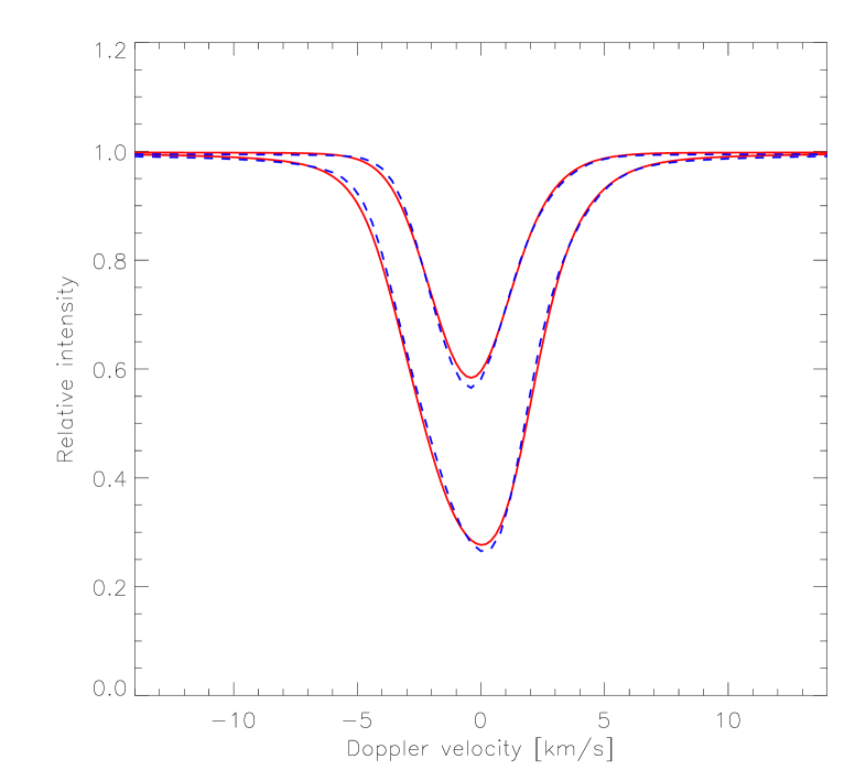
Figure 5: The predicted Fe i 608.2 (weaker) and 621.9 nm (stronger) lines at two different resolutions of the solar convection simulation: 200 x 200 x 82 (solid) and 50 x 50 x 82 (dashed). All profiles have been computed with log$\,\epsilon_{\rm Fe}=7.50$

The non-thermal broadening of spectral lines stems predominantly from the Doppler shifts due to the convective flows inherent in the granulation (e.g. Paper I). A substantial part of the total line strength of solar Fe lines is therefore contributed by the convective broadening, in particular for stronger, partly saturated, lines. The mean temperature structures in the simulations are essentially determined by mass conservation and the amount of radiative cooling at the visible surface, which should be basically independent of the numerical resolution (Stein & Nordlund 1998). As seen in Fig. 2 the temperature structures in the various 3D simulations are indeed very similar, which is also true for the average entropy structures. From this follows that the average vertical velocity is similar in the convection zone (Fig. 3) but it is not true that also the velocity distributions will be insensitive to the resolution (Stein & Nordlund 1998). In particular this is not correct in the photospheric layers which are important for the line broadening. Although the bulk of the velocity distributions only show minor differences, the high-velocity tails of the distributions are indeed quite sensitive to the resolution (Fig. 4). With a better resolution the more extreme velocities, which can contribute significant line broadening, are more likely due to the smaller effective viscosity. On the basis of such considerations, one would therefore expect the widths and strengths of weak lines to be less sensitive to the resolution while stronger, partly saturated, lines should show a higher degree of dependence. It can be noted that the vertical velocity distributions are quite symmetric in terms of up- and downflows at the visible surface and line-forming regions, while it is markedly skewed in the deeper layers, with much larger descending velocities (Stein & Nordlund 1998). In warmer stars such as F stars with more naked granulation (Nordlund & Dravins 1990; Asplund et al., in preparation) the asymmetric velocity distributions also in the photospheric layers will be manifested in the line formation.

Figure 6: The abundances derived from Fe i (upper panel) and Fe ii (lower panel) lines as a function of the excitation potential (left panel) and equivalent widths (right panel) for two different resolutions: 200 x 200 x 82 (filled circles) and 50 x 50 x 63 (open circles). The solid and dashed lines are least-square fits to the two sets of abundances. The abundances for the intermediate resolutions are not shown for clarity but generally fall in between these two cases. Note that the trends are more pronounced here than in Paper II due to the use of equivalent widths instead of profile fitting

As suspected the line widths for a given line strength increase with increasing numerical resolution, which is illustrated in Fig. 5. Since at the highest resolution the line profiles match almost perfectly the observed profiles (Paper I and II; Asplund 2000), with a lower resolution the computed lines tend to be slightly too deep and narrow for a given equivalent width. Somewhat surprisingly it was found that the additional broadening preferentially was contributed to the blue wing of the profiles. It appears that the increased number of regions with downflow velocities of $\approx 2.5$ km s^-1 with poorer resolutions largely compensate the lack of even larger redshifted velocities.

Although the lower resolution simulations do not provide all the necessary line broadening, one may hope to be able to derive elemental abundances from equivalent widths even with a limited resolution. Table 2 lists the individual abundances thus derived for the different simulations. The mean Fe abundances from the weak and intermediate strong Fe i lines are $7.48\pm 0.05,7.51\pm 0.05$, $7.52\pm 0.06$ and $7.53\pm 0.06$, in order of decreasing numerical resolution, while for the Fe ii lines the corresponding results are $7.47\pm 0.09,7.48\pm 0.09$, $7.50\pm 0.10$ and $7.51\pm 0.10$. As expected the stronger and partly saturated lines show a greater dependence on the resolution, since those lines are sensitive to the line broadening contributed by the convective Doppler shifts. As a consequence there is a more pronounced trend between line strength and the derived abundance with poorer resolution, as shown in Fig. 6, which is also reflected in an increased scatter. Even at the highest resolution there is still a minor trend present but it is further diminished when considering line profiles rather than equivalent widths (Paper II). A possible explanation for this may be that the measured Fe i equivalent widths of Blackwell et al. (1995) suffer from a slightly too high continuum placement. This would also partly explain the difference between the Blackwell et al. (1995) and Holweger et al. (1995) results for Fe i, since the former sample is more biased towards lines sensitive to the non-thermal broadening. Such a conclusion is supported by the smaller trend for Fe ii lines (Fig. 6) with equivalent widths taken from Hannaford et al. (1992). We expect that the remaining trends will vanish further at an even higher resolution in the simulation but there may also be an influence from departures from LTE for the intermediate strong lines (Paper II); we note that no trend is apparent for Si i or Fe ii lines at the present best resolution (Asplund 2000, Paper II).

The very strong Fe i lines with pronounced damping wings on the other hand show a very small variation between the different simulations, which follows naturally by the robustness of the photospheric temperature and gas pressure structure and thus the collisional broadening. In terms of abundances the differences between the various simulations only amount to $\la 0.02$ dex. Strong lines are therefore well suited for accurate log $g$ determinations (e.g. Edvardsson 1988; Fuhrmann et al. 1997) using simulations of even very modest resolution, due to the consistent results in terms of abundances derived from weak and strong Fe i lines (Paper II).

According to common wisdom the Balmer line strengths in late-type stars are essentially a diagnostic of the atmospheric temperature structure (e.g. Gray 1992), since the pressure-sensitivity of the Stark-broadening cancels the pressure-dependence on the number of H^- ions in the ratio of line opacity to continuous opacity, leaving the necessary excitation of H i as a probe of the temperature structure. Given the immunity of the mean temperature to the resolution, in particular in the relevant line-forming layers (Fig. 2), one would therefore expect the wings of the Balmer lines to be independent to such details. It does not come as a surprise then that the predicted H$\alpha$ and H$\beta$ lines are indeed identical in the different simulations. Hydrogen lines can therefore with confidence be employed for more realistic $T_{\rm eff}$ determinations based on 3D simulations even of very limited resolution, provided of course that the theoretical (atomic) H broadening is properly understood (Barklem et al. 2000a).

4.3 Effects on line shifts and asymmetries

Figure 7: The predicted bisectors for the Fe i 608.2 (Upper panel) and 621.9 nm (Lower panel) lines at different resolutions of the solar convection simulation: 200 x 200 x 82 (solid), 100 x 100 x 82 (dotted), 50 x 50 x 82 (dashed) and 50 x 50 x 63 (dot-dashed). All profiles have been computed with log$\,\epsilon_{\rm Fe}=7.50$. Since with the highest resolution the theoretical bisectors agree almost perfectly with the observed bisectors (Paper I) it is clear that an insufficient resolution produces discrepant line asymmetries

The departures from perfect symmetry in the spectral line profiles reflect the convective motion and the temperature-velocity correlations in the line-forming region and thus serve as sensitive probes of the detailed photospheric structure. For the Sun, spectral line bisectors have characteristic $\subset$-shapes although weaker lines only show the upper part of the $\subset$. At the currently best available numerical resolution (200 x 200 x 82) the predicted solar line shifts and asymmetries agree very well in general with observations (Paper I), which therefore lends very strong support for the realism of the solar convection simulations.

The differences in vertical velocities (Figs. 3 and 4) at different numerical resolutions manifest themselves in slight but noticeable differences in the predicted line shifts and asymmetries, as exemplified in Fig. 7. Although the overall bisector shapes are similar, the details are not. In particular the lowest resolution simulation produces deviant bisectors, while the intermediate cases resemble more closely the results obtained with the highest resolution. It therefore seems like the simulations have nearly converged in terms of detailed line asymmetries. The differences in predicted bisectors compared to the best case amount to $\la 200$ m s^-1 for the 50 x 50 x 63 simulation. $\la 150$ m s^-1 for the 50 x 50 x 82 simulation and $\la 50$ m s^-1 for the 100 x 100 x 82 simulation. In particular the disagreement is largest at line center and close to the continuum, which also means that in order to predict accurate stellar line shifts ($\la 50$ m s^-1) a high numerical resolution ($\sim 100^{3}$) for the 3D convection simulations is necessary. The remaining discrepancies in the cores of strong lines even at the highest resolution is most likely due to the influence from the outer boundary or possibly departures from LTE (Paper I). It should be remembered, however, that at the heights where the cores of such strong lines are formed the convection simulations are likely the least realistic due to missing ingredients, such as departures from LTE, influence of magnetic fields and additional radiative heating due to strong Doppler-shifted lines.

Figure 8: The differences between predicted and observed Fe i line bisectors for different resolutions in the 3D solar convection simulations: a: 200 x 200 x 82, b: 100 x 100 x 82, c: 50 x 50 x 82, and d: 50 x 50 x 63

Fig. 8 shows the differences between the predicted and observed bisectors for the Fe i lines in Table 2 for the various 3D resolutions. Systematic shortcomings are apparent for the poorer resolution but the situation gradually improves with higher resolutions. In particular for the most extensive simulation, most predicted bisectors agree very nicely with the observed line asymmetries (the increased scatter close to the continuum is due to the influence of weak blends). The inclusion of additional Fe i lines corroborate this conclusion (Paper I). Clearly both a high vertical and horizontal resolution is necessary to have accurate predictions in terms of line asymmetries.

5 Comparison between 2D and 3D

5.1 Effects on continuum intensity contrast

The restriction to 2D forces the over-turning motion to take place only in one horizontal direction rather than two, which in turn produces different typical length scales and convective velocities in the photosphere compared to 3D. According to Fig. 1 the granular scales are slightly larger in 2D as a result of the larger horizontal pressure fluctuations (Ludwig et al., in preparation), which also implies that the intensity contrast will be different relative to the 3D case in order to maintain the larger spatial scales. The 2D, $I_{\rm rms}$ is notably larger than for the corresponding 3D simulation even with the same effective viscosity (i.e. the same horizontal resolution dx): 17.5% and 16.6%, respectively. This difference partly explains the discrepant line asymmetries in 2D, as shown in Sect. 5.3.

5.2 Effects on line shapes and abundances

Figure 9: Upper panel: The mean temperature structure in solar convection simulations of different number of dimensions: 3D (solid) and 2D (dotted). Lower panel: The temperature difference in the sense 3D-2D, i.e. the temperatures tend to be higher in 2D in the deeper layers and lower in the optically thin regions

Figure 10: The time-averaged mean vertical velocity (upper panel) and horizontal rms vertical velocity (lower panel) in solar convection simulations of different number of dimensions: 3D (solid) and 2D (dotted). Positive vertical velocities correspond to downflows

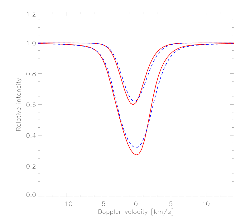
Figure 11: The predicted Fe i 608.2 (weaker) and 621.9 nm (stronger) lines at different number of dimensions of the solar convection simulation: 3D (solid) and 2D (dashed). The individual Fe abundances have been adjusted according to Table 2 to produce the same equivalent widths in 2D and 3D

Due to the smaller computational demands posed by 2D convection simulations and radiative transfer computations compared to corresponding 3D calculations, it is of interest to compare the effects of number of dimensions on the predicted spectral line profiles. Since the temperature and velocity structures depend on the number of dimensions as seen in Figs. 9 and 10, it can not be assumed that the predicted line shapes and strengths will be the same in 2D and 3D. The restriction to 2D facilitates a more efficient merging of down-flows. This produces larger horizontal scales in 2D (Fig. 1, which is associated with larger horizontal pressure fluctuations and thus different vertical velocity structures. The details of the differences in the temperature structures are more subtle but are related to the velocity variations; cf. Ludwig et al., in preparation, for a detailed discussion on the physical reasons for the differences in convection properties between 2D and 3D.

Fig. 11 shows a couple of theoretical 2D and 3D Fe i lines computed with the Fe abundances given in Table 2 to return the same equivalent widths; the Fe ii lines show the same behaviour and discrepancies. Although the overall line shape (but not the detailed line asymmetries and shifts as discussed in Sect. 5.3) is relatively similar for weaker Fe i lines, the profiles of intermediate strong lines are very different, with the 2D profiles being much shallower and broader than the corresponding 3D profiles. Since in 3D the predicted lines agree almost perfectly with observations (Paper I and Paper II), it implies that the agreement is relatively poor in 2D. In particular, even at very high resolution in 2D abundance analyses would have to be restricted to using equivalent widths rather than profile fitting due to the inherent shortcomings of the 2D predictions. Likewise, with 2D analyses too low projected rotational velocities of the stars would be obtained due to the too broad predicted line profiles.

Figure 12: The abundances derived from Fe i (upper panel) and Fe ii lines (lower panel) as a function of the excitation potential (left panel) and equivalent widths (right panel) for different number of dimensions of the convection simulations: 3D (filled circles) and 2D (open circles). The solid and dashed lines are least-square fits to the two sets of abundances. The trend with line strength is more pronounced here than in Paper II due to the use of equivalent widths instead of profile fitting and lower numerical resolution

In terms of derived abundances the 2D and 3D results show systematic differences. The sample of Fe i lines in Table 2 give mean Fe abundances of $7.51\pm 0.05$ (3D: 100 x 100 x 82) and $7.41\pm 0.06$ (2D: 100 x 82). The corresponding results for the Fe ii lines are $7.48\pm 0.09$ (3D) and $7.51\pm 0.10$ (2D). The remaining difference in mean $T_{\rm eff}$ of 36 K between the 2D and 3D case translates to an abundance difference for Fe i and Fe ii of -0.03 and +0.01 dex, respectively. The larger difference between the 2D and 3D cases for Fe i lines is a natural consequence of the greater sensitivity to the temperature structure for those lines. The derived 2D Fe abundances show essentially identical trends with equivalent widths and excitation potential, as seen in Fig. 12; the differences in the Fe i results are basically restricted to a systematic offset of about 0.1 dex for all lines. With the current best solar simulation (the 200 x 200 x 82 simulation used here) and profile fitting instead of equivalent widths, neither the Fe i nor the Fe ii lines show any significant trends with excitation potential, and only Fe i lines depend slightly on line strengths, which may reflect departures from LTE rather than shortcomings of the convection simulations as such (Paper II).

Strong Fe i lines with pronounced pressure damped wings can be efficient gravitometers (e.g. Edvardsson 1988; Fuhrmann et al. 1997), provided the collisional broadening is properly understood (Anstee & O’Mara 1991, 1995; Barklem & O’Mara 1997; Barklem et al. 1998, 2000b). Due to differences in pressure and temperature structures, the predicted strong lines are indeed quite different in 2D compared to in 3D, with the 2D lines being stronger for a given abundance. While in 3D the strong Fe i lines imply abundances consistent within 0.05 dex of those of weak and intermediate strong lines (Paper II), in 2D the strong lines suggest abundances systematically about 0.10 dex lower than those of weaker lines. This naturally translates to significant errors when estimating stellar surface gravities from the wings of strong lines using 2D convection simulations.

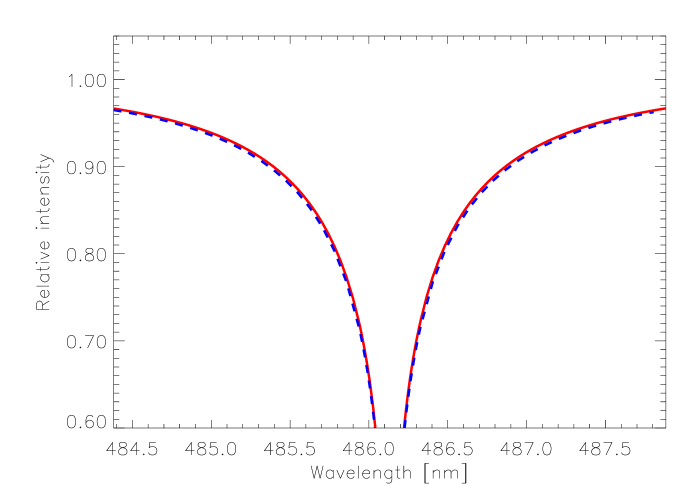
Figure 13: The temporally and spatially averaged H$\beta$ profile computed using the 3D (solid line) and 2D (dashed line) solar convection simulations. In spite of the existing temperature differences (Fig. 9), the spatially averaged H$\beta$ profiles are very similar in 2D and 3D

In 3D the H lines are effectively independent on the chosen resolution as discussed above. When comparing 2D with 3D the same conclusion does not follow automatically since the convective transport properties and therefore temperature structures are different, as illustrated in Fig. 9 and discussed in detail by Ludwig et al., in preparation. The temperature difference is notably larger between 2D and 3D than for different numerical resolution in 3D (Fig. 2). As seen in Fig. 13 the resulting Balmer H$\beta$ profiles are however very similar, albeit with minor differences in the near wing, with the 2D profile being slightly broader than in 3D, in accordance with the somewhat steeper temperature gradient (Fig. 9). Since in terms of $T_{\rm eff}$ the difference only amounts to about 30 K, an accurate $T_{\rm eff}$ calibration using Balmer lines should be possible with 2D convection simulations, provided the remaining problems with the theoretical (atomic) H line broadening can be addressed (Barklem et al. 2000a).

5.3 Effects on line shifts and asymmetries

The atmospheric temperature inhomogeneities and macroscopic velocity fields produce characteristic spectral line asymmetries, which for solar-type stars take on $\subset$-shaped bisectors. Since both the temperatures and flow pattern are different in 2D than in 3D (Figs. 9 and 10), the predicted bisectors will depend on the adopted number of dimensions of the convection simulations, which is illustrated in Fig. 14 for a couple of Fe i lines. Although the overall bisector shapes are qualitatively similar the detailed line asymmetries are not, neither for weak nor intermediate strong Fe i and Fe ii lines. The predicted line shifts from the 2D simulation are less blue-shifted by typically 100-200 m s^-1 compared with the corresponding 3D estimates for weak lines, although the differences vanish for stronger lines with cores formed above the granulation layers. Due to the complex interplay between temperature inhomogeneities, velocity fields and brightness contrasts in producing the line asymmetries, it is very difficult to identify which difference in the physical variables is most responsible for the bisector variations, but it is clear that at least the quite different convective velocities play an important role, since the deceleration zone occurs over a larger vertical extent with different amplitude of the vertical velocities, as seen in Fig. 10.

The discrepancies are even larger closer to the continuum, amounting to as much as 300 m s^-1, as evident in Fig. 15 which shows the differences between theoretical and observed solar Fe i line bisectors for the corresponding 2D and 3D simulations. It should be noted that the time coverages are sufficient for both the 2D and 3D simulations (16.5 hrs and 50 min, respectively) to produce statistically significant spatially and temporally averaged bisectors, as verified by test calculations restricted to much shorter time sequences: half the time interval produces indistinguishable bisectors from the full calculations, while shorter sequences covering 10% of the whole simulation stretches have an accuracy of $\la 100$ m s^-1 due to the influences of granular evolution and the radial oscillations corresponding to the solar 5-min oscillations which are present in the numerical box. Furthermore, the blue-most bend in the bisectors also occur at significantly larger line-depths in 2D than in 3D, again reflecting the shortcomings when simulating a 3D phenomenon like convection in 2D. Since the most realistic 3D predictions agree very well with the observed bisectors it is clear that 2D results are significantly less accurate.

Figure 14: The predicted bisectors for the Fe i 608.2 (weaker) and 621.9 nm (stronger) lines at different number of dimensions of the solar convection simulation: 3D (solid) and 2D (dashed). The individual Fe abundances have been adjusted according to Table 2 to produce the same equivalent widths in 2D and 3D. Since in 3D the theoretical bisectors agree almost perfectly with the observed bisectors (Paper I) it is clear that 2D simulations produce discrepant line asymmetries. Note that all bisectors are on an absolute wavelength scale, emphasizing the shortcomings of the 2D simulations to accurately predict the line shifts

Figure 15: The differences between predicted and observed Fe i line bisectors for 3D (Upper panel) and 2D (Lower panel) solar convection simulations. In 2D neither the line asymmetries nor the line shifts are accurately described

6 Conclusions

The aim of the present paper has been to investigate how sensitive predicted line profiles and bisectors are to the adopted numerical resolution and number of dimensions of the convection simulations used as model atmospheres in the line transfer calculations. The investigations have been performed strictly differentially in order to isolate the effects of the dimensions of the numerical grid.

The numerical resolution in 3D has a limited influence on the theoretical line profiles and asymmetries. With a too coarse resolution the lines tend to be slightly too narrow and deep, but at the highest resolution we have used to date the predictions have converged almost perfectly to the observed values, both in terms of line shapes and asymmetries, which lend strong support to the realism of the convection simulations. In terms of abundances, weak lines show a small dependence on resolution ($\simeq 0.02$ dex) while intermediate strong lines with their larger sensitivity to the non-thermal Doppler broadening show a greater dependence ($\la 0.10$ dex). Both for the intention of deriving accurate elemental abundances and using line asymmetries as probes of stellar surface convection, a resolution of $\simeq 100^{3}$ appears sufficient considering the observational uncertainties in stellar spectroscopy today ($\la 0.05$ dex and $\la 100$ m s^-1, respectively). On the other hand, strong lines of Fe i and H are only marginally affected by the resolution, since they mainly reflect the atmospheric temperature and pressure structures which converge already at very modest resolution, as a natural consequence of mass conservation (Stein & Nordlund 1998). Therefore, accurate $T_{\rm eff}$ and log $g$ calibrations can be achieved even with a grid of 3D convection simulations of very limited resolution.

Unfortunately 2D convection simulations appear less reliable for abundance analyses and studies of line asymmetries, since the inherent convective transport properties are different in 2D compared to in 3D. The predicted line profiles in 2D are too shallow and broad for a given line strength, in particular for intermediate strong lines which are sensitive to the convective velocity broadening. As a consequence, the agreement with observed profiles is far from satisfactory. Furthermore, the derived abundances are not immune either to the adopted number of dimensions of the convection simulation, in particular for the Fe i lines. The same conclusion holds when comparing line asymmetries and shifts with differences amounting to $\ga 200$ m s^-1 on an absolute velocity scale. Even the coarsest 3D resolution investigated here (50 x 50 x 63) produces more realistic results in general than corresponding 2D simulations in terms of line strengths and asymmetries. In light of the findings presented here and in Paper I, one may conclude that some of the claims of a good correspondence between observations and 2D predictions (e.g. Gadun et al. 1999) are probably fortuitous. The right results can be obtained for the wrong reasons if shortcomings in terms of e.g. resolution, equation-of-state, opacities, depth scale, and temperature structure compensate the errors introduced by the restriction to 2D rather than treating convection fully in 3D.

Also for an additional reason, 2D convection simulations provide less of an attractive approach compared to 3D than at first glance when considering the computational demand. Due to the poorer spatial coverage of the surface convection, the time variations are significantly larger in 2D than in 3D. As a consequence, correspondingly longer time sequences are needed in order to obtain statistically significant averaged convection properties and line profiles. Rather than a difference of a factor of about 100 (assuming typical numerical grids of $100^{3}$ and $100^{2}$, respectively, mesh points) in computing time, in practice only a factor of $\la 5$ is more likely saved. Given the limitations found here in terms of spectral line formation, the difference is hardly of great importance, in particular since more realistic 3D simulations are affordable today even with normal work-stations.

Table 2: Atomic data and derived abundances for Fe lines using 3D and 2D convection simulations

Species	Wavelength	log $gf$	$\chi_{\rm l}$	$W_{\lambda}$	log $\epsilon_{\rm Fe}$	log $\epsilon_{\rm Fe}$	log $\epsilon_{\rm Fe}$	log $\epsilon_{\rm Fe}$	log $\epsilon_{\rm Fe}$a
	[nm]		[eV]	[pm]	($200^{2}{\rm x}82$)	($100^{2}{\rm x}82$)	($50^{2}{\rm x}82$)	($50^{2}{\rm x}63$)	($100{\rm x}82$)
Fe i	438.92451	-4.583	0.052	7.17	7.46	7.53	7.56	7.55	7.40
	444.54717	-5.441	0.087	3.88	7.44	7.46	7.45	7.45	7.34
	524.70503	-4.946	0.087	6.58	7.46	7.52	7.53	7.53	7.39
	525.02090	-4.938	0.121	6.49	7.47	7.52	7.54	7.53	7.39
	570.15444	-2.216	2.559	8.51	7.55	7.59	7.61	7.62	7.50
	595.66943	-4.605	0.859	5.08	7.46	7.49	7.49	7.49	7.38
	608.27104	-3.573	2.223	3.40	7.45	7.47	7.46	7.47	7.38
	613.69946	-2.950	2.198	6.38	7.41	7.45	7.46	7.47	7.37
	615.16182	-3.299	2.176	4.82	7.41	7.44	7.43	7.45	7.36
	617.33354	-2.880	2.223	6.74	7.44	7.48	7.49	7.50	7.40
	620.03130	-2.437	2.608	7.56	7.55	7.60	7.61	7.62	7.51
	621.92808	-2.433	2.198	9.15	7.49	7.53	7.54	7.55	7.42
	626.51338	-2.550	2.176	8.68	7.47	7.52	7.53	7.54	7.42
	628.06182	-4.387	0.859	6.24	7.46	7.50	7.51	7.51	7.39
	629.77930	-2.740	2.223	7.53	7.46	7.50	7.52	7.53	7.42
	632.26855	-2.426	2.588	7.92	7.58	7.63	7.64	7.65	7.54
	648.18701	-2.984	2.279	6.42	7.49	7.53	7.54	7.55	7.45
	649.89390	-4.699	0.958	4.43	7.46	7.49	7.48	7.49	7.38
	657.42285	-5.004	0.990	2.65	7.42	7.43	7.41	7.42	7.31
	659.38706	-2.422	2.433	8.64	7.54	7.58	7.59	7.60	7.48
	660.91104	-2.692	2.559	6.55	7.49	7.53	7.54	7.55	7.45
	662.50220	-5.336	1.011	1.36	7.39	7.40	7.38	7.38	7.27
	675.01523	-2.621	2.424	7.58	7.50	7.54	7.56	7.57	7.46
	694.52051	-2.482	2.424	8.38	7.50	7.55	7.56	7.57	7.45
	697.88516	-2.500	2.484	8.01	7.50	7.55	7.56	7.57	7.45
	772.32080	-3.617	2.279	3.85	7.52	7.54	7.53	7.54	7.46
					$7.48\pm 0.05$	$7.51\pm 0.05$	$7.52\pm 0.06$	$7.53\pm 0.06$	$7.41\pm 0.06$
Fe ii	457.63334	-2.940	2.844	6.80	7.47	7.51	7.55	7.56	7.53
	462.05129	-3.210	2.828	5.40	7.39	7.42	7.46	7.47	7.44
	465.69762	-3.590	2.891	3.80	7.45	7.47	7.49	7.50	7.48
	523.46243	-2.230	3.221	8.92	7.50	7.53	7.55	7.56	7.53
	526.48042	-3.250	3.230	4.74	7.61	7.63	7.66	7.67	7.66
	541.40717	-3.500	3.221	2.76	7.38	7.39	7.40	7.41	7.41
	552.51168	-3.950	3.267	1.27	7.40	7.41	7.41	7.41	7.43
	562.74892	-4.100	3.387	0.86	7.46	7.46	7.47	7.47	7.50
	643.26757	-3.500	2.891	4.34	7.40	7.42	7.44	7.45	7.45
	651.60767	-3.380	2.891	5.75	7.58	7.61	7.63	7.64	7.64
	722.23923	-3.360	3.889	2.00	7.59	7.60	7.60	7.61	7.64
	722.44790	-3.280	3.889	2.07	7.53	7.54	7.55	7.55	7.58
	744.93305	-3.090	3.889	1.95	7.30	7.30	7.31	7.31	7.32
	751.58309	-3.440	3.903	1.49	7.50	7.50	7.51	7.51	7.55
	771.17205	-2.470	3.903	5.06	7.42	7.44	7.46	7.47	7.48
					$7.47\pm 0.09$	$7.48\pm 0.09$	$7.50\pm 0.10$	$7.51\pm 0.10$	$7.51\pm 0.10$