X–ray Emission of Mkn 421: New Clues From Its Spectral Evolution.
I. Temporal Analysis

Abstract

Mkn 421 was repeatedly observed with BeppoSAX in 1997–1998. This is the first of two papers where we present the results of a thorough temporal and spectral analysis of all the data available to us, focusing in particular on the flare of April 1998, which was simultaneously observed also at TeV energies. Here we focus on the time analysis, while the spectral analysis and physical interpretation are presented in the companion paper. The detailed study of the flare in different energy bands reveals very important new results: i) hard photons lag the soft ones by 2–3 ks – a behavior opposite to what is normally found in high energy peak BL Lacs X–ray spectra; ii) the flare light curve is symmetric in the softest X–ray band, while it becomes increasingly asymmetric at higher energies, with the decay being progressively slower than the rise; iii) the flux decay of the flare can be intrinsically achromatic if a stationary underlying emission component is present. The temporal and spectral information obtained challenge the simplest models currently adopted for the (synchrotron) emission and most importantly provide clues on the particle acceleration process.

1. Introduction

Blazars are radio–loud AGNs characterized by strong variability, large and variable polarization, and high luminosity. Radio spectra smoothly join the infrared-optical-UV ones. These properties are successfully interpreted in terms of synchrotron radiation produced in relativistic jets and beamed into our direction due to plasma moving relativistically close to the line of sight (e.g. Urry & Padovani up95, 1995). Many blazars are also strong and variable sources of GeV $\gamma$–rays, and in a few objects the spectrum extends up to TeV energies. The hard X– to $\gamma$–ray radiation forms a separate spectral component, with the luminosity peak located in the MeV–TeV range.

The emission up to X–rays is thought to be due to synchrotron radiation from high energy electrons in the jet, while it is likely that $\gamma$-rays derive from the same electrons via inverse Compton (IC) scattering of soft (IR–UV) photons –synchrotron or ambient soft photons (e.g. Sikora, Begelman & Rees sbr94, 1994, Ghisellini et al. gg_sed98, 1998).

The contributions of these two mechanisms characterize the average blazar spectral energy distribution (SED), which typically shows two broad peaks in a $\nu F_{\nu}$ representation (e.g. von Montigny et al. vmon95, 1995; Sambruna, Maraschi & Urry smu96, 1996; Fossati et al. 1998a, ): the energies at which the peaks occur and their relative intensity provide a powerful diagnostic tool to investigate the properties of the emitting plasma, such as electron energies and magnetic field (e.g. Ghisellini et al. gg_sed98, 1998). Moreover variability studies, both of single band and of simultaneous multifrequencies data, constitute the most effective means to constrain the emission mechanisms at work in these sources as well as the geometry and modality of the energy dissipation. The quality and amount of X–ray data on the brightest sources start to allow us to perform a thorough temporal analysis as function of energy and determine the spectral evolution with good temporal resolution.

In X–ray bright BL Lacs (HBL, from High-energy-peak-BL Lacs, Padovani & Giommi pg95, 1995) the synchrotron maximum (usually) occurs in the soft-X–ray band, and the inverse Compton emission extends in some cases to the TeV band where – thanks to ground based Cherenkov telescopes – four sources have been detected up to now: Mkn 421 (Punch et al. punch92, 1992), Mkn 501 (Quinn et al. quinn96, 1996), 1ES 2344+514 (Catanese et al. catanese_2344_98, 1998), and PKS 2155–304 (Chadwick et al. chadwick98, 1998). If the interpretation of the SED properties in terms of synchrotron and IC radiation is correct, a correlation between the X–ray and TeV emission is expected.

Mkn 421 ($z$ = 0.031) is the brightest BL Lac object at X–ray and UV wavelengths and the first extragalactic source discovered at TeV energies, where dramatic variability has been observed with doubling times as short as 15 minutes (Gaidos et al. gaidos96, 1996). As such it was repeatedly observed with X–ray satellites, including BeppoSAX. Remarkable X–ray variability correlated with strong activity at TeV energies has been found on different occasions (Macomb et al. macomb95, 1995, 1996, Takahashi et al. takahashi96, 1996, Fossati et al. 1998b, , Maraschi et al. maraschi_letter, 1999). In particular, the 1998 BeppoSAX data presented here were simultaneous with a large TeV flare detected by the Whipple Observatory (Maraschi et al. maraschi_letter, 1999).

This paper is the first of two, which present the results of a uniform, detailed spectral and temporal analysis of BeppoSAX observations of Mkn 421 performed during 1997 and 1998. Here we focus on the data reduction and the timing analysis, and also discuss the results on the spectral variability derived from the different properties of the flux variations in different energy bands.

The paper is organized as follows. We briefly summarize the characteristics of BeppoSAX (§2), and introduce the observations studied (§3). We then address the temporal analysis of the variability, considering several energy bands and comparing the light curve features by means of a few simple estimators for the 1997 and 1998 observations (§4). The remarkable flare observed in 1998 is the object of a further deeper analysis, reported in Section §5, focused on timescales and time lags. Section 6 contains a summary of the results of the temporal analysis, preparing the ground for the comprehensive discussion presented in Paper II (Fossati et al. fossati_II, 2000). There they are considered together with the results of the spectral analysis and thus used to constrain a scenario able to interpret the complex spectral and temporal findings.

2. BeppoSAX overview

For an exhaustive description of the Italian/Dutch BeppoSAX mission we refer to Boella et al. (boella97, 1997) and references therein. The narrow field coaligned instrumentation (NFI) on BeppoSAX consists of a Low Energy Concentrator Spectrometer (LECS), three Medium Energy Concentrator Spectrometers (MECS), a High Pressure Gas Scintillation Proportional Counter (HPGSPC), and a Phoswich Detector System (PDS). The LECS and MECS have imaging capabilities in the 0.1–10 keV and 1.3–10 keV energy band, respectively, with energy resolution of 8% at 6 keV. At the same energy, the angular resolution is about 1.2 arcmin (Half Power Radius). In the overlapping energy range the MECS effective area (150 cm²) is $\sim$ 3 times that of the LECS. Furthermore the exposure time for the LECS is limited by stronger operational constraints to avoid UV light contamination through the entrance window (LECS instrument is operated during Earth dark time only). The HPGSPC covers the range 4–120 keV, and the PDS the range 13–300 keV. In the overlapping interval the HPGSPC has a better energy resolution than the PDS, but it is less sensitive of both PDS and MECS. Therefore, HPGSPC data will not be discussed in this paper.

The present analysis is based on the SAXDAS linearized event files for the LECS and the three MECS experiments, together with appropriate background event files, as produced at the BeppoSAX Science Data Center (rev 0.2, 1.1 and 2.0). The PDS data reduction was performed using the XAS software (Chiappetti & Dal Fiume chiappetti_dalfiume, 1997) according to the procedure described in Chiappetti et al. (chiappetti_2155, 1999).

3. Observations

Mkn 421 has been observed by BeppoSAX in the springs of 1997 and 1998. The journal of observations is given in Table 1.

3.1. 1997

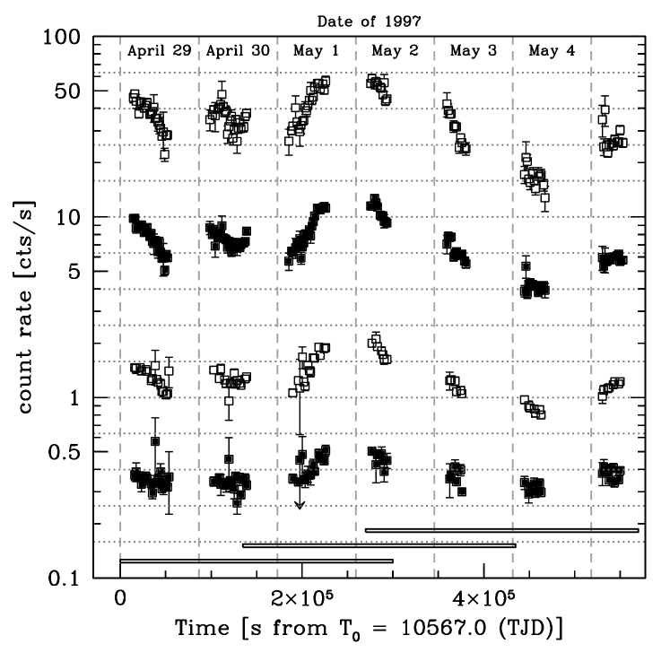
The 1997 observation comprised several pointings spanning the interval between April 29^th and May 7^th. MECS data are not available for May 7^th because of the failure of the detector unit 1 on May 6^th. In this paper we will not consider the LECS data of this last day of the 1997 campaign, because unfortunately LECS data alone do not provide useful spectral and variability information. The net exposure time (excluding the May 7^th data) was $\sim$ 52 and $\sim$ 117 ks for LECS and MECS respectively, while the on–source time coverage computed as the sum of the observations between each T_start and T_stop is of about 58 hr.

Results on the first half of the 1997 campaign (April 29^th to May 1^st) have been presented by Guainazzi et al. (guainazzi_mkn421, 1999), where the details and motivation of the observations are given. We re–analyzed those data along with the new ones, applying the same techniques, in order to obtain a homogeneous set of results, necessary for a direct comparison.

Table 1Journal of Observations

Date (UTC)			Net Exposure Time (ks)				BeppoSAX archive #
Start	Stop		LECS	MECS	PDS
1997/04/29:04:02	1997/04/29:14:42		11.6	21.8	18.4		50032001
1997/04/30:03:19	1997/04/30:14:42		11.4	24.1	23.0		50032002
1997/05/01:03:17	1997/05/01:14:42		11.2	23.8	22.8		50032003
1997/05/02:04:10	1997/05/02:09:41		04.4	11.4	11.0		50016002
1997/05/03:03:24	1997/05/03:09:41		04.3	11.7	11.2		50016003
1997/05/04:03:25	1997/05/04:09:45		04.9	12.2	11.6		50016004
1997/05/05:03:32	1997/05/05:09:45		05.0	11.9	11.4		50016005
1997/05/07:04:47	1997/05/07:10:27		06.0	$\cdots$	13.1		50016006
1998/04/21:01:52	1998/04/22:03:13		23.6	29.6	42.2		50686002
1998/04/23:00:27	1998/04/24:06:37		27.2	34.7	50.4		50686001

3.2. 1998

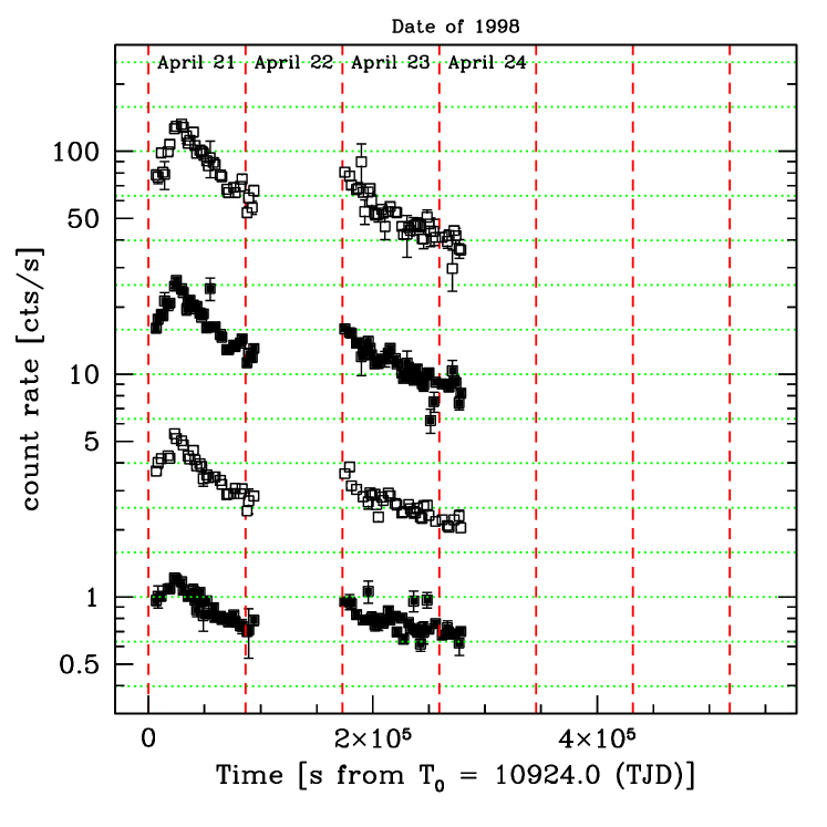
In 1998 BeppoSAX observed Mkn 421 as part of a long monitoring campaign involving BeppoSAX, ASCA (Takahashi, Madejski, & Kubo takahashi99_veritas, 1999), RossiXTE (Madejski et al., in preparation), and coverage from ground based TeV observatories (Maraschi et al. maraschi_letter, 1999). The BeppoSAX observation comprised two distinct long pointings, started respectively on April 21^st and 23^rd. The total net exposure time for MECS telescopes has been of 64 ks and the LECS one adds up to 50 ks. Hereinafter we will refer to the two 1998 pointings simply as April 21^st and April 23^rd, leaving out the year.

The actual on–source time was 55.5 hr. Unfortunately celestial and satellite constraints in late April 1998 were such that in each orbit there are two intervals during which the reconstructed attitude is undefined. One occurs when the source is occulted by the dark Earth, but the second longer one occurs during source visibility periods. Thus there are about 19 min per orbit when the NFIs are pointing at the source, but there is a gap in attitude reconstruction despite the high Earth elevation angle. During these intervals the source position is drifting along the $\pm$X detector axis, from a position in the center to about 12 arcmin off, passing the strongback window support. These intervals are excluded by the LECS/MECS event file generation. Using the XAS software it is possible to accumulate MECS images also during such intervals, showing that the source is actually drifting. The drift causes a strong energy dependent modulation, clearly visible in light curves accumulated with XAS, and which would be very difficult to recover, as requires to build a response matrix integrated from different position dependent matrices weighted according to the time spent in each position. We then did not try to recover these data for the analysis.

In the case of PDS the source remains inside the collimator flat–top during the drift, and therefore we used for the accumulation all events taken when the Earth elevation angle was greater than 3 degrees (inclusive of attitude gaps).

4. Temporal Analysis

Light curves have been accumulated for different energy bands. The input photon lists were extracted from the full dataset selecting events in a circular region centered on the position of the point source. The extraction radii are 8 and 6 arcmin for LECS and MECS respectively, chosen to be large enough to collect most of the photons in the whole energy range: the used values ensure that $<$ 5 % of the photons are missed, at all energies.

For MECS data we considered the merged photon list of all the available MECS units, which were 3 for the 1997 observations and only 2 (namely MECS units 2 and 3) in 1998.

The expected background contribution is less than a fraction of a percent (typically of the order of 0.2–0.5 %) and therefore the light curves have not been background subtracted.

In order to maximize the information on the spectral/temporal behavior, the choice of energy bands shall be such that they are as independent as possible. This should take into account the instrumental efficiencies and, at a certain level, the details of the spectral shape. The main trade–off is the number of photons in each band, that should be large enough to obtain statistically meaningful results. Taking into account the main features of the LECS and MECS effective areas (e.g. the Carbon edge at 0.29 keV which provides with independent energy bands below and above this energy) and the steepness of the Mkn 421 spectrum (above a few keV the available photons quickly become insufficient), we determined the following bands: 0.1–0.5 keV and 0.5–2 keV for LECS data, 2–3 and 4–6 keV for MECS data. Their respective “barycentric” energies are 0.26, 1.16, 2.35, 4.76 keV, respectively, thus providing a factor $\sim 20$ leverage, useful to test the energy dependence of the variability characteristics.

4.1. 1997

The four resulting light curves for 1997 are presented in Figure 1. The source shows a high degree of flux variability, with possibly a major flare between the third and fourth pointings. The vertical scale is logarithmic allowing a direct comparison of the amplitude of variations at different energies. As anticipated we are not going to consider further the LECS data of May 7^th, however for sake of completeness we report that the count rate was of 0.37$\pm$0.01 and 1.06$\pm$0.04 cts/s for the 0.1–0.5 and 0.5–2.0 keV energy bands respectively, comparable to the level measured on May 5^th.

The comparison of data with the overlaid reference grid shows that the amplitude of variability is larger at higher energies, as commonly observed in blazars at energies above the SED peak (e.g. Ulrich, Maraschi & Urry umu97, 1997). We will discuss this issue more quantitatively in section §4.3.

Figure 1.— Light curves in four energy bands for the 1997 observations. They are shown in order of decreasing energy from top to bottom: 4–6 keV (multiplied by a factor 100), 2–3 keV (multiplied by a factor 10), 0.5–2 keV, 0.1–0.5 keV. The binning time is 1500 s. The reference time TJD=10567.0 corresponds to 1997–April–29:00:00 UT. The horizontal bars shown at the bottom of the plot mark the time intervals considered for the analysis of the variability properties in §4.3: subset–1 to –3 from left to right.

Figure 2.— Light curves in four energy bands for the 1998 observations. They are shown in order of decreasing energy from top to bottom: 4–6 keV (multiplied by a factor 100), 2–3 keV (multiplied by a factor 10), 0.5–2 keV, 0.1–0.5 keV. The binning time is 1500 s. The reference time TJD=10924.0 corresponds to 1998–April–21:00:00 UT. In order to allow an easier comparison with the 1997 light curves, the X scale has been expanded to the same length of that of Figure 1, and also the Y–axis dynamic range is the same.

Figure 3.— Light curves at TeV and X–ray energies, during the 1998 campaign. They are shown in order of decreasing energy from top to bottom: Whipple E$\geq$ 2 TeV, (multiplied by a factor 500), PDS 12–26 keV (one point per orbit, multiplied by a factor 50), MECS 4–6 keV (multiplied by a factor 5) and LECS 0.1–0.5 keV (both with 1500 s bins). The count rate units are cts/s for BeppoSAX data, and cts/min for Whipple data. The thicker dashed grid marks the days, while the thinner ones have a 20 ks spacing. TJD=10924.0 corresponds to 1998–April–21:00:00 UT.

4.2. 1998

The 1998 light curves are shown in Figure 2, (see the caption for details about the axis scales). The overall appearance is somewhat different, being dominated by a single isolated flare at the beginning of the campaign. The variability amplitude is similar to the 1997 one in each corresponding energy band (see also §4.3).

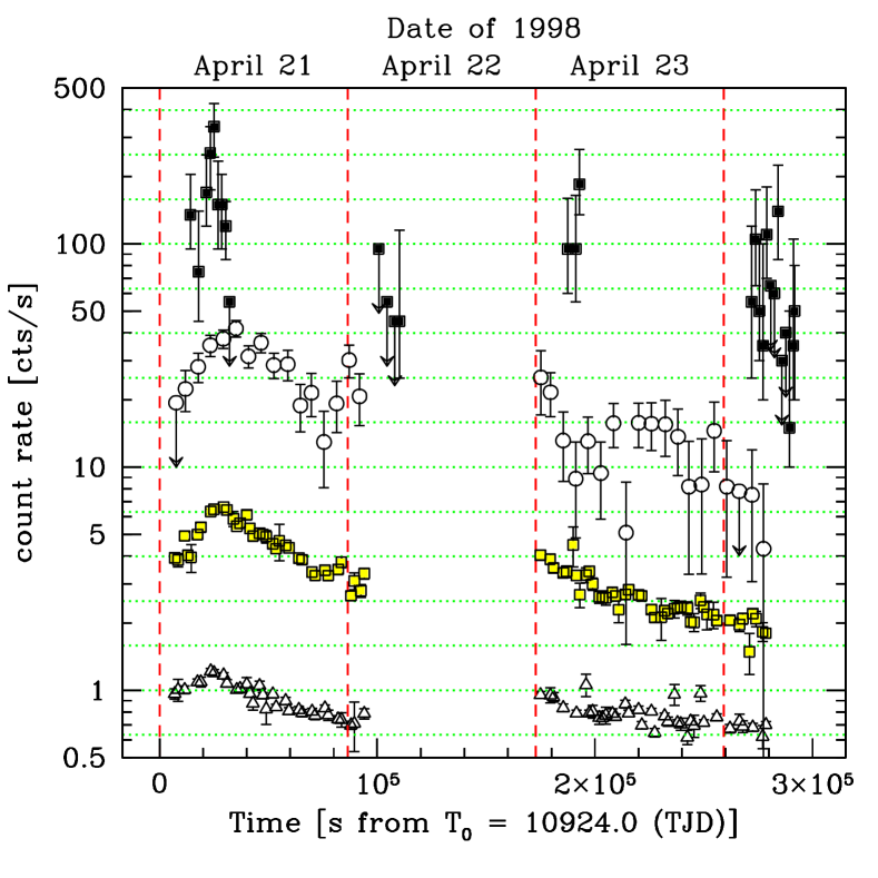
The most striking and important result of the campaign is that in correspondence with the X–ray flare of April 21^st a sharp TeV flare was detected by the Whipple Cherenkov Telescope, with amplitude of a factor 4 and a halving time of about 2 hr (Maraschi et al. maraschi_letter, 1999). In Figure 3 the Whipple TeV (E$\geq$2 TeV) light curve is shown together with the BeppoSAX ones: LECS (0.1–0.5 keV), MECS (4–6 keV) and PDS (12–26 keV) instruments. The peaks in the 0.1–0.5 keV, 4–6 keV and 2 TeV light curves are simultaneous within one hour. Note however that the TeV variation appears to be both larger and faster than the X–ray one. The 12–26 keV light curve shows a broader and slightly delayed peak with respect to lower energy X–rays. However the very limited statistics does not allow us to better quantify this event. A more detailed account on this particular result is presented and discussed by Maraschi et al. (maraschi_letter, 1999).

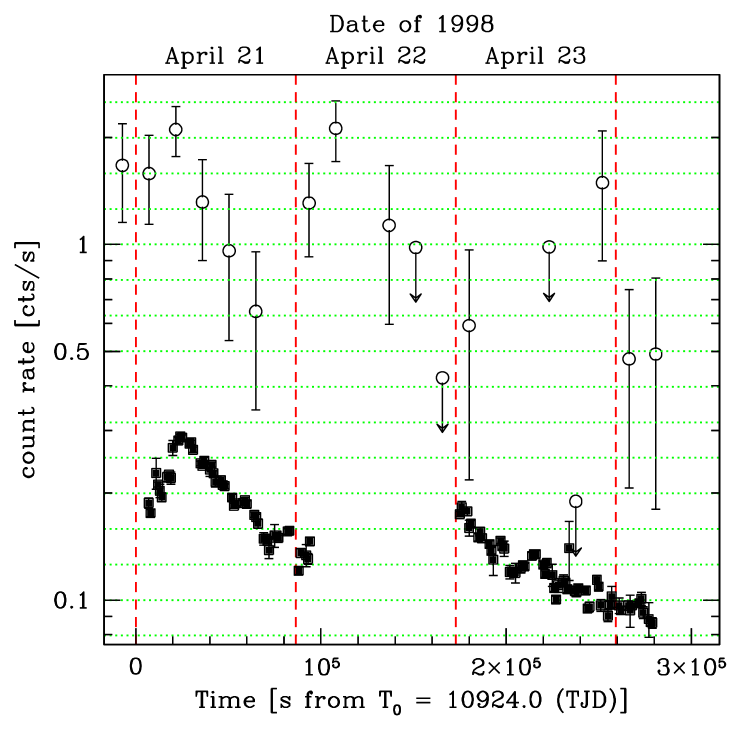
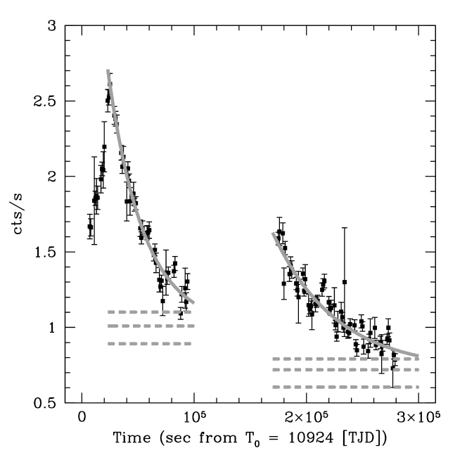
It is also worth noticing that the positive (flux) offset of the beginning of April 23^rd with respect to the end of the April 21^st suggests the presence of a second flare occurring between the two pointings. This seems to be also confirmed by the RossiXTE All Sky Monitor (ASM) light curve, shown in Fig. 4 together with the MECS one in the (2–10 keV) nominal working energy range of the ASM. Single ASM $\sim$90 s dwells have been rebinned in 14400 s (i.e. 4 hr) intervals, weighting the contribution of each single dwell on its effective exposure time and on the quoted error. The MECS light curve bin is 1000 s. Indeed the ASM light curve appears to unveil the presence of a second flare occurring in between the two BeppoSAX pointings, with a brightness level similar to that of the detected one.

On the other hand the few Whipple data points at the time of this putative second X–ray flare (at T = (100–120) $\times 10^{3}$ s, see Figure 3) do not indicate any (major) TeV activity: the count rate measured by the Whipple telescope was in fact significantly lower than that measured simultaneously with the first X–ray flare.

Figure 4.— RossiXTE All Sky Monitor light curve (top) compared with the MECS in the same (2–10 keV) band, scaled by a factor 1/20.

4.3. Comparison of 1997 and 1998 variability characteristics

We can characterize the variability in different X–ray bands by two commonly used estimators: the fractional root mean square ($r.m.s.$) variability parameter F_var, and the minimum “doubling/halving time” T_short (for definitions and details see Appendix A, and Zhang et al. zhang_2155, 1999).

4.3.1 Fractional r.m.s. variability

For each (0.1–0.5, 0.5–2, 2–3 and 4–6 keV) band we computed F_var for the whole 1997 and 1998 datasets which have the same on–source coverage (i.e. $\sim$ 55 hr).

Moreover, for the 1997 we considered three (partially overlapping) subsets of data each spanning a time interval comparable to the length of the whole 1998 observation, i.e. $\sim$ 300 ks. The intervals cover the first 300 ks, a middle section, and the last 300 ks, as marked on Fig. 1.

For each dataset F_var is computed for 6 different light curve binning intervals, namely 200, 500, 1000, 1500, 2000 and 2500 s, and then the weighted average of these values is computed. The results are listed in Table 2 and shown in Figure 5.

Table 2Basic Variability Estimators

	LECS 0.1–0.5	LECS 0.5–2	MECS 2–3	MECS 4–6
Energy (keV)	0.26	1.18	2.36	4.76
r.m.s. variability estimator Fvar
1998 All	$0.151\pm 0.006$	$0.267\pm 0.009$	$0.315\pm 0.009$	$0.366\pm 0.011$
1997 All	$0.145\pm 0.035$	$0.215\pm 0.007$	$0.257\pm 0.020$	$0.305\pm 0.012$
1997 sub–1	$0.154\pm 0.039$	$0.189\pm 0.008$	$0.198\pm 0.014$	$0.209\pm 0.024$
1997 sub–2	$0.176\pm 0.010$	$0.282\pm 0.013$	$0.340\pm 0.012$	$0.385\pm 0.014$
1997 sub–3	$0.154\pm 0.024$	$0.289\pm 0.018$	$0.374\pm 0.015$	$0.432\pm 0.017$
shortest timescale Tshort (ks)
1997: all data	$80.6\pm 46.6$	$28.6\pm\phantom{0}6.4$	$25.5\pm 2.4$	$25.5\pm 2.0$
1997: halving	$167.4\pm 31.0\phantom{0}$	$62.9\pm\phantom{0}4.4$	$31.0\pm 3.1$	$32.6\pm 8.0$
1997: doubling	$81.7\pm 62.1$	$28.2\pm\phantom{0}6.6$	$27.3\pm 4.1$	$28.7\pm 3.4$
1998: all data	$63.8\pm 12.1$	$28.1\pm\phantom{0}4.2$	$27.3\pm 2.4$	$21.4\pm 1.5$
1998: halving	$63.8\pm 12.1$	$35.7\pm\phantom{0}4.1$	$36.9\pm 8.7$	$34.5\pm 2.4$
1998: doubling	$\cdots$	$30.4\pm 12.1$	$28.4\pm 3.3$	$23.6\pm 1.9$

Figure 5.— Plot of the root mean square variability parameter, F_var, versus energy. A small energy shift has been applied for sake of clarity.

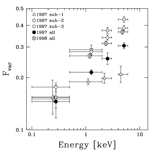
If we treat all the datasets as independent and momentarily do not consider the subset–1 of the 1997 light curve (empty triangles in Fig. 5) on which we will comment later, it appears that:

1. In terms of root mean square variability the lower energy flux is less variable than the higher energy one, as already pointed out in section §4.1. This holds independent of both the length of the time interval and the state of the source.

2. There is no relation between the brightness level and the variability amplitude, since although in 1998 the source was at least a factor 2 brighter than in 1997 the corresponding F_var are not larger.

What is different for the subset–1 of the 1997 light curve ?

First two caveats on F_var. This quantity is basically only sensitive to the average excursion around the mean flux, and does not carry any information about either duty cycle or the actual flux excursion. Therefore in order for F_var to meaningfully represent the variability, the “extrema” of the source variability have to be sampled. This is clearly not the case for the first 1997 sub–light curve (see Figure 1). Furthermore, F_var is estimated from the comparison of the variances of the light curve and the measurements, but while the latter ones probably obey a Gaussian distribution and are much smaller than the former ones, the “probability” for the source to show a significant deviation from the average (i.e. the count rate histogram distribution) is in most cases highly non–Gaussian. For a typical “flaring” light curve this has a “core” at low count rates, resulting from the long(er) time spent by the source in between flares, and a very extended tail to high(er) rates. The implicit assumption of Gaussian variability can thus affect the estimate of F_var (as for large amplitude and low duty cycle variability).

F_var is thus a particularly poor indicator especially for observations with a window function like the one of 1997, for which the source temporal covering fraction is of the same order of the single outburst, making likely to miss the flare peak, and the total span of the observation does not significantly exceed the frequency of peaks. We therefore believe this affects the results relative to the first subsample of 1997.

In order to obtain a variability estimator more sensitive to the dynamic range towards higher count rates (flaring) we also considered a modified definition of it, F_var,med: to study only the width (amplitude) of the brighter tail only data above the median count rate are considered to compute variance and expected variance. Note that the modified definition is still affected by the problem of “representativity” of all the source states. Since the median is always smaller than the average (for all energies, and for all trial time binnings), the values of F_var,med are larger than F_var, but in every other respect the results are qualitatively unchanged.

Figure 6.— (a) comparison of global T_short for 1997 (crossed squares) and 1998 (diamonds), (b) comparison of doubling (black triangles) and halving (white triangles) timescales for 1997, and (c) comparison of doubling (black squares) and halving (white squares) timescales for 1998 (see text).

4.3.2 Doubling/halving timescale

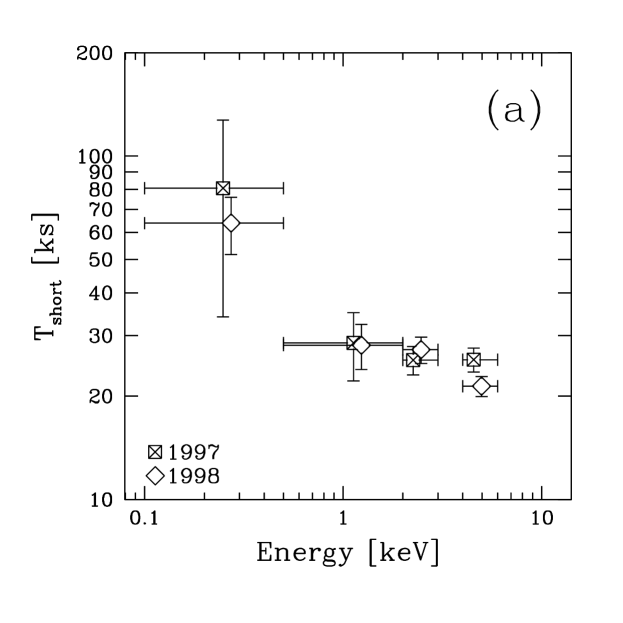
Similarly, the “minimum halving/doubling” timescale has been computed for each energy band taking the average of values for the different input light curve binning (but discarding the 200 s one because too strongly subject to spurious results). As in Zhang et al. (zhang_2155, 1999) we rejected a T_short,ij if the fractional uncertainty was larger than 20 %.

In order to minimize the contamination by isolated data points we filtered the light curves excluding data lying at more than 3-$\sigma$ from the average computed over the 6 nearest neighbors (3 on each side), and for the 500 s binning light curves we did not consider pairs between data closer than 3 positions along the time series. Finally instead of taking the single absolute minimum value of T_short,ij (over all possible $i,j$ pairs) T_short is determined as the average over the 5 lowest values.

The resulting T_short are listed at the bottom of Table 2 and shown in Figure 6a. The main findings are:

1. there is not significant difference between 1997 and 1998 observations, at any energy.

2. There is weak evidence that the softest X–ray band exhibits slower variability, while

3. the timescales for the three higher energy bands are indistinguishable, and there is no sign of a trend with energy.

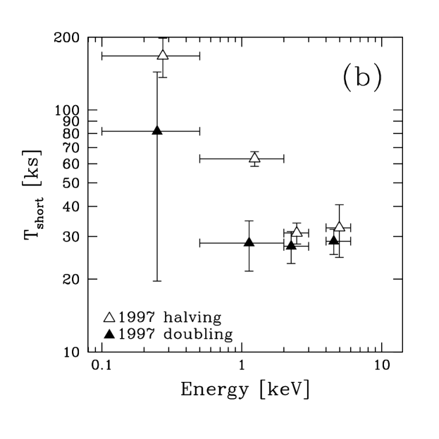
We also distinguish doubling and halving timescales. Unfortunately it has not been possible to obtain an estimate of the doubling time for the lowest energy band for 1998 data, because there are only a few, uncertain, data during the rise of the flare. We find that (see Table 2, and Figure 6b,c):

1. again the softest X–ray band shows longer (halving) timescales;

2. there is marginal evidence that the doubling timescale is shorter than the halving one (i.e. the rise is faster than the fall).

This latter result seems to hold both for 1997 and 1998 light curves and for each single trial binning time, and for each energy (except in 5 cases out of 35). However it is strongly weakened by the averaging over the several time binnings because T_short slightly increases with the duration of the time bins, thus yielding a larger uncertainty on the average.

5. 1998 detailed temporal analysis

We performed a more detailed analysis of the characteristics of the April 21^st flare, in particular to determine any significant different behavior among different energy bands. Three are the main goals: i) to measure the flare exponential (or power–law) decay timescales (or power–law index); ii) to evidence possible differences in the flare rise and decay timescales; iii) to look for time lags among the different energies.

We considered the energy ranges already adopted in Section 4.

5.1. Decay Timescales

A first estimate of the decay timescales has been presented by Maraschi et al. (maraschi_letter, 1999), where a simple exponential law has been fit to the decaying phase of the light curves, and a dependence of the e–folding timescale on the energy band has been found. Here we analyze the issue of determining the timescale in more detail and in particular we consider the requirement for the presence of an underlying steady emission.

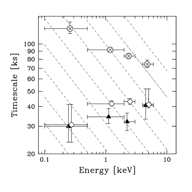
In particular, the decay timescales for different energy bands have been estimated by fitting the post–flare light curves with an exponential decay superimposed to a constant (quasi–steady) flux eventually constrained by the fit (we immediately stress that an additional non–zero steady emission is necessary in order to obtain a meaningful fit with an exponential decay). In one set of fits the underlying contribution is set to zero. More precisely, we performed the fits with three possible conditions for the level of the steady contribution: un–constrained, constrained and zero.

The analytical expression of the function used in the fits is:

$$\mathrm{F}(t) \;=\; \mathrm{F}_{\mathrm{steady}}+\mathrm{F}_{\mathrm{flaring}}\;e^{-\frac{\mathrm{t}\;-\;\mathrm{T}_{\mathrm{ref}}}{\tau}}$$

$$\;=\; \mathrm{F}_{\mathrm{steady}}\;\left(1+{\cal R}\;e^{-\frac{\mathrm{t}\;-\;\mathrm{T}_{\mathrm{ref}}}{\tau}}\right)$$

The model parameters are then the decay timescale $\tau$, the absolute value of F_steady, and the ratio ${\cal R}$ between the flaring and the steady component taken at a reference time T_ref, which ideally should correspond to the peak of the flare.

The “reference time” T_ref for April 21^st flare was T${}_{\mathrm{ref}}=25\times 10^{3}$ s (T$=0=10924.0$ TJD), and T${}_{\mathrm{ref}}=170\times 10^{3}$ s for April 23^rd. Note that the value of ${\cal R}$ obtained from the fit to the second dataset is only a lower limit on the actual flare amplitude since we do not have an estimate of the time at which the peak of this putative second flare occurred.

In any case, as our focus is actually on the properties of the first, well defined, outburst, we used the parameters obtained from the April 23^rd data only to constrain the contribution from the steady component. Furthermore, it turns out that the determination of the timescale $\tau$ is not affected by the uncertainty on its contribution (see Table 3 and Fig. 8).

We adopted a 1000 s binning for the 0.5–2 keV and 2–3 keV data, which have better statistics, while we the binning time for the 0.1–0.5 keV and 4–6 keV light curves is of 2000 and 1500 s, respectively. The analysis has been performed in two stages, for each energy band:

• Fit to the April 21^st and 23^rd datasets independently, yielding values of $\tau$, F_steady and ${\cal R}$. As an example, in Figure 7 the 2–3 keV light curve is shown together with its best fit models for April 21^st and 23^rd.

• Fit of the April 21^st post–flare phase constraining the level of the underlying steady component to be below the level of April 23^rd (the actual constraint is the upper bracket for a two parameters 90% confidence interval). We assume that the underlying emission varies on a timescale longer than that spanned by the observations.

As anticipated we also modeled the decay of the April 21^st flare setting to zero the offset.

The results are summarized in Tables 3 and 4. The best fit $\tau$ for all the three cases are plotted in Fig. 8 as a function of energy.

The 0.1–0.5 keV timescale is not affected by the constraint on the baseline flux and the 4–6 keV confidence interval only suffers a minor cut (smaller errorbar), while both the 0.5–2 and 2–3 keV parameters are significantly changed because the best fit un–constrained level of the steady contribution is significantly higher than allowed by the April 23^rd data (see for instance Fig. 7).

Figure 7.— Example of the fit of the light curve with a constant+exponential decay. The 2–3 keV data are shown, with a 1000 s time bin, together with the best fit model (solid line through the data points), and the best fit level of the steady component (three dashed lines corresponding to the best fit value and the 90% confidence interval, for two interesting parameters).

Table 3Parameters of fit to light curves

		LECS 0.1–0.5	LECS 0.5–2	MECS 2–3	MECS 4–6
constant + exponential decay
April 21, zero–baseline
$\tau$	(ks)	125.3${}^{+8.6}_{-5.8}$	91.8${}^{+1.9}_{-1.5}$	83.8${}^{+1.8}_{-2.2}$	74.4${}^{+3.1}_{-2.3}$
April 21, un-constrained
${\cal R}$		00.77${}^{+0.24}_{-0.13}$	01.38${}^{+0.19}_{-0.15}$	01.58${}^{+0.22}_{-0.16}$	02.97${}^{+3.01}_{-0.77}$
Fsteady	(cts/s)	00.68${}^{+0.05}_{-0.08}$	02.23${}^{+0.12}_{-0.18}$	01.01${}^{+0.07}_{-0.09}$	00.39${}^{+0.09}_{-0.12}$
$\tau$	(ks)	29.9${}^{+11.4}_{\phantom{0}-6.2}$0	34.4${}^{+4.5\phantom{0}}_{-3.2}$0	32.1${}^{+4.3\phantom{0}}_{-4.0}$0	40.7${}^{+11.1}_{\phantom{0}-7.4}$0
April 21, constrained
${\cal R}$		00.77${}^{+0.24}_{-0.13}$	01.66${}^{+0.11}_{-0.04}$	02.19${}^{+0.16}_{-0.04}$	02.97${}^{+3.01}_{-0.49}$
Fsteady	(cts/s)	00.67-0.07	01.94-0.07	00.79-0.03	00.39-0.12
		[$<$ 0.72]	[$<$ 1.94]	[$<$ 0.79]	[$<$ 0.39]
$\tau$	(ks)	30.7${}^{+10.6}_{\phantom{0}-6.9}$0	41.7${}^{+1.8\phantom{0}}_{-1.2}$0	43.0${}^{+2.0\phantom{0}}_{-1.7}$0	41.2${}^{+10.6}_{\phantom{0}-1.9}$0
April 23, un-constrained
${\cal R}$		00.38${}^{+0.09}_{-0.07}$	00.95${}^{+0.27}_{-0.13}$	01.25${}^{+0.24}_{-0.16}$	01.35${}^{+0.17}_{-0.11}$
Fsteady	(cts/s)	00.70${}^{+0.02}_{-0.04}$	01.77${}^{+0.16}_{-0.24}$	00.72${}^{+0.06}_{-0.08}$	00.36${}^{+0.03}_{-0.03}$
$\tau$	(ks)	29.0${}^{+22.0}_{-10.3}$0	66.6${}^{+21.1}_{-13.3}$0	55.6${}^{+14.0}_{\phantom{0}-9.1}$0	39.2${}^{+8.6\phantom{0}}_{-6.0}$0
constant + power law decay
${\cal R}$		$>$ 1.715	$>$ 15.15	$>$ 23.04	$>$ 39.37
Fsteady	(cts/s)	$<$ 0.600	$<$ 0.619	$<$ 0.489	$<$ 0.175
$\eta$		0.54${}^{+0.37}_{-0.18}$	0.54${}^{+0.05}_{-0.02}$	0.62${}^{+0.16}_{-0.02}$	0.70${}^{+0.09}_{-0.03}$

Table 4Timescales for Different Exponential Decay Fits

		LECS 0.1–0.5	LECS 0.5–2	MECS 2–3	MECS 4–6
April 21, zero–baseline
T${}_{\mathrm{end}}=100\times 10^{3}$		125.3${}^{+8.6}_{-5.8}$	91.8${}^{+1.9}_{-1.5}$	83.8${}^{+1.8}_{-2.2}$	74.4${}^{+3.1}_{-2.3}$
T${}_{\mathrm{end}}=\phantom{0}90\times 10^{3}$		120.3${}^{+8.2}_{-5.7}$	89.0${}^{+2.0}_{-1.5}$	80.3${}^{+2.4}_{-1.7}$	72.0${}^{+3.7}_{-2.0}$
T${}_{\mathrm{end}}=\phantom{0}80\times 10^{3}$		116.2${}^{+9.0}_{-6.1}$	84.9${}^{+2.0}_{-1.7}$	73.8${}^{+2.6}_{-1.8}$	68.5${}^{+3.8}_{-2.4}$
T${}_{\mathrm{end}}=\phantom{0}70\times 10^{3}$		106.2${}^{+7.8}_{-5.9}$	80.7${}^{+2.0}_{-1.9}$	70.8${}^{+2.5}_{-2.1}$	68.5${}^{+3.4}_{-3.0}$
T${}_{\mathrm{end}}=\phantom{0}60\times 10^{3}$		095.3${}^{+9.5}_{-6.6}$	76.0${}^{+2.7}_{-2.1}$	70.0${}^{+3.6}_{-2.8}$	70.3${}^{+5.9}_{-4.1}$
${\cal P}$		$4\times 10^{-2}$	$6\times 10^{-8}$	$1\times 10^{-5}$	$\cdots$
April 21, un-constrained baseline
T${}_{\mathrm{end}}=100\times 10^{3}$		029.9${}^{+11.4}_{\phantom{0}-6.2}$	34.4${}^{+4.5}_{-3.2}$	32.1${}^{+4.3}_{-4.0}$	40.7${}^{+11.1}_{\phantom{0}-7.4}$
T${}_{\mathrm{end}}=\phantom{0}90\times 10^{3}$		033.8${}^{+14.8}_{\phantom{0}-8.4}$	37.7${}^{+5.5}_{-4.1}$	34.0${}^{+5.6}_{-4.7}$	46.3${}^{+16.5}_{-10.4}$
T${}_{\mathrm{end}}=\phantom{0}80\times 10^{3}$		026.9${}^{+10.9}_{\phantom{0}-7.1}$	34.5${}^{+5.6}_{-4.8}$	38.6${}^{+10.4}_{\phantom{0}-7.5}$	53.6${}^{+19.6}_{-16.9}$
T${}_{\mathrm{end}}=\phantom{0}70\times 10^{3}$		032.3${}^{+24.0}_{-11.1}$	34.6${}^{+9.7}_{-5.7}$	45.6${}^{+26.5}_{-12.5}$	61.7${}^{+12.0}_{-26.3}$
T${}_{\mathrm{end}}=\phantom{0}60\times 10^{3}$		032.6${}^{+70.4}_{-14.3}$	26.3${}^{+8.0}_{-5.0}$	24.2${}^{+11.2}_{\phantom{0}-5.9}$	18.9${}^{+14.4}_{\phantom{0}-6.2}$
${\cal P}$		$\cdots$	$\cdots$	$\cdots$	$\cdots$
April 21, constrained baseline
T${}_{\mathrm{end}}=100\times 10^{3}$		030.7${}^{+10.6}_{\phantom{0}-6.9}$	41.7${}^{+1.8}_{-1.2}$	43.0${}^{+2.0}_{-1.7}$	41.2${}^{+10.6}_{\phantom{0}-1.9}$
T${}_{\mathrm{end}}=\phantom{0}90\times 10^{3}$		033.3${}^{+15.1}_{\phantom{0}-8.0}$	41.2${}^{+3.4}_{-1.3}$	42.0${}^{+3.0}_{-1.5}$	46.2${}^{+16.6}_{\phantom{0}-7.2}$
T${}_{\mathrm{end}}=\phantom{0}80\times 10^{3}$		026.6${}^{+11.3}_{\phantom{0}-3.4}$	40.8${}^{+3.3}_{-1.2}$	40.6${}^{+8.9}_{-1.7}$	53.1${}^{+19.4}_{-14.3}$
T${}_{\mathrm{end}}=\phantom{0}70\times 10^{3}$		031.9${}^{+24.4}_{\phantom{0}-8.8}$	40.5${}^{+6.1}_{-1.4}$	345.5${}^{+26.2}_{\phantom{0}-7.1}$	63.5${}^{\phantom{0}+9.3}_{-24.4}$
T${}_{\mathrm{end}}=\phantom{0}60\times 10^{3}$		032.7${}^{+69.3}_{\phantom{0}-9.4}$	40.2${}^{+5.0}_{-1.8}$	41.5${}^{+9.6}_{-2.4}$	44.3${}^{+23.0}_{\phantom{0}-3.9}$
${\cal P}$		$\cdots$	$\cdots$	$\cdots$	$\cdots$

Figure 8.— Decay timescales $\tau$ plotted versus the barycentric energy of the data from which they have been derived. The different symbols are: crossed circles for zero–baseline, black triangles for the un–constrained baseline, and diamonds for the constrained baseline case. The dashed lines show the loci of the relation $\tau\sim\mathrm{E}^{-1/2}$, that holds if pure radiative cooling is responsible for the spectral variability during the burst decay.

The main findings are:

• the decay timescales depend critically on the presence/ absence of a contribution by a non variable component. This is true not only for the value themselves (for the case without baseline are between a factor 2 and 4 longer) but also for the relationship between the timescales and energy. In fact:

  • In the cases with baseline, the timescales range between 30 and 45$\times 10^{3}$ s, and do not show a clear (if any) relationship with the energy, rather suggesting an achromatic post–flare evolution. In fact, according to a $\chi^{2}$ test, the values of $\tau$ for the 4 energies are consistent with coming from the same distribution (the so called “null hypothesis”).

  • On the contrary, in the case of pure exponential decay the timescales follow a weak inverse relationship with the energy, $\tau\propto E^{-0.18\pm 0.02}$ (both when considering $\tau$ or $E$ as the dependent variable). The $\chi^{2}$ probability in favor of the “null hypothesis” is in this case negligible.

• the amplitude of the variability (as measured by ${\cal R}$) positively correlates with the energy, as reported in many cases for HBLs (e.g. Sambruna et al. sambruna_exosat, 1994, Ulrich et al. umu97, 1997).

5.1.1 Is there a steady component ?

Variability timescales and their energy dependence carry precious information on the physics of the source: the puzzling dependence of the results on the hypothesis of the presence of a steady component requires further analysis.

Here we only discuss a simple test of the robustness of the results of previous section, that however provides useful hints. This consists in determining $\tau$ for different choices of the end time (T_end) of the interval over which the fit is performed. The underlying idea is that if the shape of the decay is close to the one we are assuming (exponential with/without an offset) one can expect that the model parameters do not change much as a function of T_end. On the contrary, if the chosen model provides only a poor description of the actual decay characteristics, the parameters will likely take different values depending on T_end, unless of course we postulate a process whose timescale changes with time.

For each of the three cases (constrained, unconstrained, zero–baseline) we tried 5 different choices of the end time, namely T${}_{\mathrm{end}}=60$, 70, 80, 90 and 100$\times 10^{3}$ seconds (from T₀), the last one corresponding to the entire duration of the data coverage on April 21^st.

To evaluate the likelihood that the 5 values of $\tau$ obtained for these choices of T_end are drawn from the same (normal) distribution, we considered the probability ${\cal P}$ of the $\chi^{2}$ computed with respect to their weighted average.

In Table 4 we summarize the results obtained under each of the different hypotheses. There are a few points to note:

1. in the zero–baseline hypothesis the timescales obtained changing T_end are not consistent with being several different realizations from a unique distribution. Furthermore the clear trend of (decreasing) $\tau$ with (decreasing) T_end supports the possibility that the variation of $\tau$ is significant.

2. On the contrary in both cases with baseline the values of $\tau$’s for the 0.1–0.5, 0.5–2 and 2–3 keV bands are very close for all values of T_end. For the 4–6 keV band the scatter is somewhat larger, likely due to the fact that at this energy there is the largest amplitude of variability, i.e. the smallest contribution of the putative baseline. The same kind of effect of lowered sensitivity to the details of a putative baseline, is responsible for the good result of the 4–6 keV band in the case without baseline.

3. Even in the case without baseline the values of $\tau$ for the various energy bands become very similar for T${}_{\mathrm{end}}=60\times 10^{3}$ s. Therefore even if the failure of the test by the pure exponential decay model could be interpreted as the signature of a mechanism whose characteristic timescale changes with time (unlike a true exponential decay), there is anyway an indication that in the earlier stages of the decay the evolution is not energy dependent.

On the basis of this simple consistency check we can therefore infer that if the decay were exponential there is evidence for the presence of an underlying non–variable component. Thus the post–flare phase does not show any dependence on energy, and the timescale is of the order of 30–40 ks.

Figure 9.— Index of the power law decay plotted versus energy. Only the value for the April 21 post peak decay is plotted.

5.2. Power Law Decay

As an alternative description of the decay of April 21^st flare we consider a power law, where F${}_{\mathrm{flaring}}\propto(\mathrm{T}/\mathrm{T}_{\mathrm{ref}})^{-\eta}$, again leaving the possibility of an offset from a steady component. The results are summarized in Table 3 and Figure 9.

A fundamental difference with respect to the exponential decay case is that an additional steady component is never required: the power law fits yield only (not very stringent) upper limits on F_steady and only for the 0.1–0.5 keV band the formal best fit value for F_steady is different from zero (F${}_{\mathrm{steady}}=0.26$ cts/s).

Again there is only a weak relationship of the decay properties with energy, with a marginal indication that the flux decrease is faster at higher energies. The values for the 4 energy bands are consistent with a common (weighted average) value of $\eta=0.583$, while for the subset comprising only the three higher energy datasets the probability for the “null hypothesis” is reduced to about 0.07.

5.3. Rise vs. Fall

A further interesting question is whether the rise and the decay phases of the flare are characterized by the same timescale (i.e. if the flare is symmetric or asymmetric) and in particular how these properties might correlate with energy.

The observational coverage of the rise is not good enough to apply the same direct technique used for the decay (§5.1), to constrain the timescale of an exponential rise, with all the parameters left free. Thus the flux level of the steady component is fixed at the best fit value obtained for the decay, or set to 0.

Table 5Difference between Rise and Fall Timescales

case		LECS 0.1–0.5	LECS 0.5–2	MECS 2–3	MECS 4–6	${\cal P}$
F${}_{\mathrm{steady}}=0$		2.9${}^{+33.4}_{-12.3}$	26.3${}^{+15.0}_{\phantom{0}-3.4}$	33.1${}^{+11.2}_{\phantom{0}-2.5}$	38.6${}^{+4.8}_{-3.4}$	$\cdots$
Fsteady best fit un-constrained		1.2${}^{+6.9\phantom{0}}_{-4.3}$	13.7${}^{+4.3\phantom{0}}_{-1.9}$	14.8${}^{+7.9\phantom{0}}_{-1.3}$	23.6${}^{+8.5}_{-1.9}$	$3\times 10^{-2}$
Fsteady best fit constrained		1.3${}^{+6.2\phantom{0}}_{-4.3}$	16.1${}^{+6.3\phantom{0}}_{-2.1}$	19.8${}^{+10.9}_{\phantom{0}-1.6}$	24.6${}^{+9.1}_{-2.2}$	$1\times 10^{-2}$

Figure 10.— Difference between the post–peak decay and the pre–peak rise timescales, plotted versus energy. The different symbols are: crossed circles for F${}_{\mathrm{steady}}=0$ case, black triangles for the F_steady set at the best fit value of the un–constrained case, and diamonds for F_steady set at the best fit value obtained for the April 23^rd data (see Table 3).

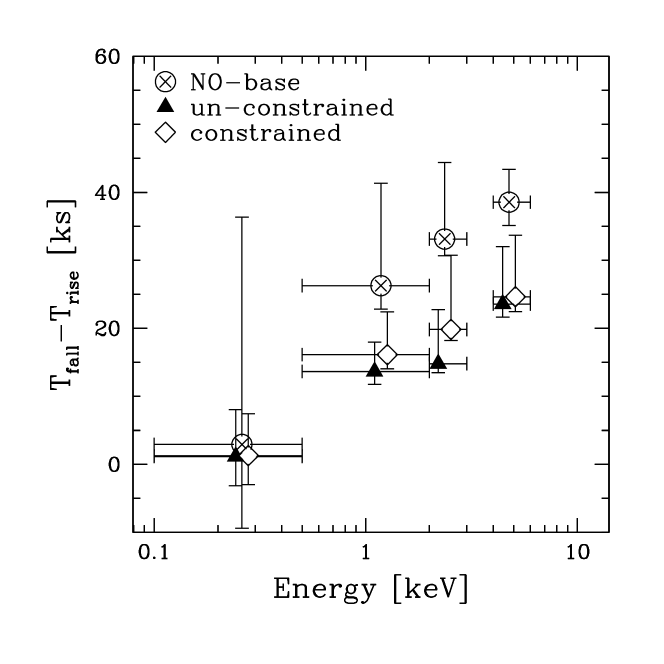
We are mainly interested in the comparison of the properties of the outburst just before and after the top of the flare (see discussion in Paper 2), and the interval of about 17–18 ks preceding the flare is long enough for this purpose.

We thus focused on the “tip” of the flare, considering data on the decay side only up to the time when the flux reaches approximately the level at which the observation starts. The duration of the post–peak intervals needed to decrease the flux to the pre–flare level are of about 15–20, 25, 30–35 and 40 ks for the four energy bands. Since the uncertainties on the decay time of the light curves are not larger than 5 ks, the differences in duration and the trend (longer time at higher energy) are real.

The differences between rise and fall timescales, estimated with fits to the light curves, are shown in Table 5, and plotted in Figure 10. The flare is symmetric for the softest energy band, while it is definitely asymmetric in the other three bands, with an asymmetry which appears to increase systematically with energy: at higher energies the rise phase is increasingly faster than the decay (the significance is reported in Table 5).

It is worth stressing that these numbers indicate only relative changes in the timescales before and after the peak of the flare. On the other hand, since we found that the decay timescales are very similar once the baseline flux is taken into account (§5.1), this asymmetry probably means that the rise times get shorter with increasing energy.

5.4. Time Lag

We performed a detailed cross correlation analysis using two different techniques suited to unevenly sampled time series: the Discrete Correlation Function (DCF, Edelson & Krolik edelson_krolik88, 1988) and the Modified Mean Deviation (MMD, Hufnagel & Bregman hufnagel_bregman92, 1992). Moreover, Monte Carlo simulations, taking into account ”flux randomization” (FR) and ”random subset selection” (RSS) of the data series (see Peterson et al. peterson_etal98, 1998), were used to statistically determine the significance of the time lags between different X–ray bands obtained with the DCF and MMD. We refer for the relevant details of such analysis to Zhang et al. (zhang_2155, 1999).

Figure 11.— Result of the cross–correlation DCF method applied to the 0.1–1.5 and 3.5–10 keV light curves. Negative values corresponds to the 3.5–10 keV band lagging the 0.1–1.5 keV one. The continuous curve superimposed to the data is the best fit with a constant$+$Gaussian model. The actual fit has been performed only to the “core” of the data, i.e. taking into account the data in the interval ranging from $-$30000 to 30000 seconds.

Figure 12.— Cross Correlation Peak Distributions for the FR/RSS simulations. The solid line is for the analysis with DCF technique, and the dashed for the case of MMD. Negative values corresponds to the 3.5–10 keV band lagging the 0.1–1.5 keV one.

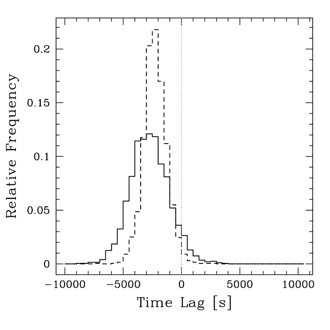
We binned the light curves over 300 s in the 0.1–1.5 and 3.5–10 keV bands (whose effective barycentric energies are E $\simeq 0.8$ and E $\simeq 5$ keV), and a trial time step of 720 s is adopted for both the DCF and MMD. DCF amplitude versus time lag is plotted in Figure 11. A negative value means that variations in the 3.5–10 keV band light curve lag those occurring in the 0.1–1.5 keV one (i.e. hard lag). The best Gaussian fits for both DCF and MMD result in negative time lags of $-2.8\pm 0.2$ (DCF) and $-2.1\pm 0.3$ (MMD) ks, indicating that the medium energy X–ray photons lag the soft ones.

The Cross Correlation Peak Distribution (CCPD) obtained from the FR/RSS Monte Carlo simulations is shown in Figure 12 both for the DCF and the MMD methods. The average lags resulting from CCPD are $-2.7^{+1.9}_{-1.2}$ ks for DCF, and $-2.3^{+1.2}_{-0.7}$ ks for MMD (1 $\sigma$ confidence intervals, two sided with respect to the average), confirming the significance of the above results with high ($>$ 90 %) confidence.

The total integral probabilities for a negative lag (that would be the actual measure of the confidence of the “discovery” of the hard lag) are $\simeq 95.0$% (DCF) and $\simeq 98.7$% (MMD).

6. Summary of Variability Properties

We presented a comprehensive temporal analysis of the flux variability characteristics in several energy bands, of BeppoSAX observations of Mkn 421. The primary results of this study are the following:

1. The fractional r.m.s. variability is higher at higher energies.

2. The fractional r.m.s. variability does not change with the brightness state of the source.

3. The minimum halving/doubling time is longer for the softest energy band.

4. The minimum halving/doubling time at a given energy does not change with the brightness state of the source.

5. There is a hint that the doubling timescale is shorter than the halving timescale.

The findings 1 and 2, on F_var, confirm the well known (although not fully explained) phenomenology of HBLs (see Ulrich et al. umu97, 1997 and references therein).

The results on the variability timescales (findings 3, 4, 5) show good agreement with those found with the more thorough analysis of the 1998 flare, that can be summarized as:

1. The flare decay is consistent with being achromatic, both if modeled as an exponential decay with an additional contribution from a steady component and in the case of a power law decay.

2. The results on timescales are at odds with the simplest possibility of interpreting the decay phase, i.e. that it is driven by the radiative cooling of the emitting electrons. This would give rise, in the simplest case, to a dependence of the timescale on energy, $\tau\sim\mathrm{E}^{-1/2}$. The tracks corresponding to this relationship are overlaid to the data in Fig. 8, and it is clear that they can not be reconciled.

3. The harder X–ray photons lag the soft ones, with a delay of the order of few ks. This finding is opposite to what is normally found in the best monitored HBL where the soft X–rays lag the hard ones (e.g. Takahashi et al. takahashi96, 1996 for Mkn 421; Urry et al. urry_2155, 1993, Zhang et al. zhang_2155, 1999, and Kataoka et al. kataoka_2155, 2000 for PKS 2155–304; Kohmura et al. kohmura, 1994 for H0323$+$022). The latter behavior is usually interpreted in terms of cooling of the synchrotron emitting particles.

4. Possible asymmetry in the rise/decay phases: the flare seems to be symmetric at the energies corresponding (roughly) to the peak of the synchrotron component (see the spectral analysis in Paper II), while it might have a faster rise at higher energies. This could be connected to the observed hard–lag.

5. Finally, the characteristics of the April 21^st flare suggest the presence of a quasi–stationary emission contribution, which seems to be dominated by a highly variable peaked spectrum.

7. Conclusions

BeppoSAX has observed Mkn 421 in 1997 and 1998. We analyzed and interpreted the combined spectral and temporal evolution in the X–ray range. During these observations the source has shown a large variety of behaviors, providing us a great wealth of information, but at the same time revealing a richer than expected phenomenology.

In this paper we have presented the first part of the analysis, focused on the study of the variability properties.

The fact that the higher energy band lags the softer one (with a delay of the order of 2–3 ks) and the energy dependence of the shape of the light curve during the flare (with faster flare rise time at higher energies) provide strong constraints on any possible time dependent particle acceleration mechanism. In particular, if we are indeed observing the first direct signature of the ongoing particle acceleration, progressively “pumping” electrons from lower to higher energies, the measure of the delay between the peaks of the light curves at the corresponding emitted frequencies would provide a tight constraint on the timescale of the acceleration process.

The decomposition of the observed spectrum into two components (a quasi stationary one and a peaked, highly variable one) might allow us to determine the nature and modality of the energy dissipation in relativistic jets.

In Paper II we complement these findings with those of the time resolved spectral analysis and develop a scenario to interpret the complex spectral and temporal phenomenology.

Appendix A A. Definitions of F_var and T_short

The fractional $r.m.s.$ variability amplitude is a useful parameter to characterize the variability in unevenly sampled light curves. It is defined as the square root of the so called excess variance (e.g., Nandra et al. nandra_97, 1997). This parameter, also known as the true variance (Done et al. done_92, 1992), is computed by taking the difference between the variance of the overall light curve and the variance due to measurement error, normalized by dividing by the average squared flux (count rate).

We consider a dataset $F_{i}(t_{i})$ ($i=1,N$), with an uncertainty $\sigma_{i}$ assigned to each point.

The fractional r.m.s. variability parameter is then defined as:

$$\mathrm{F}_{\mathrm{var}}\;\equiv\;\frac{\left(\sigma^{2}_{F}-\Delta^{2}_{F}\right)}{\langle F\rangle}^{1/2},$$ (A1)

where

$$\sigma^{2}_{F} \;\equiv\; \frac{1}{N-1}\;\sum_{i=1}^{N}(F_{i}-\langle F\rangle)^{2}$$ (A2)

$$\Delta^{2}_{F} \;\equiv\; \frac{1}{N}\;\sum_{i=1}^{N}\sigma_{i}^{2}.$$ (A3)

The definition of the “shortest variability timescale” is the following:

$$\mathrm{T}_{\mathrm{short}} \;\equiv\; \min_{\forall i,j}(\mathrm{T}_{\mathrm{short},ij})$$ (A4)

$$\mathrm{T}_{\mathrm{short},ij} \;\equiv\; \left|\frac{F_{ij}\;\Delta T_{ij}}{\Delta F_{ij}}\right|,$$ (A5)

where $F_{ij}\;\equiv\;(F_{i}+F_{j})/2$, $\Delta F_{ij}\;\equiv\;F_{i}-F_{j}$, and $\Delta T_{ij}\;\equiv\;T_{i}-T_{j}$.

References

- (1) Boella, G., Butler, R. C., Perola, G. C., Piro, L., Scarsi, L., & Bleeker, J. A. M. 1997, A&AS, 122, 299
- (2) Catanese, M., et al. 1998, ApJ, 501, 616
- (3) Chadwick, P. M., et al. 1998, ApJ, 513, 161
- (4) Chiappetti, L., et al. 1999, ApJ, 521, 552
- (5) Chiappetti, L., & Dal Fiume, D. 1997, in Proc. of the 5th Workshop, Data Analysis in Astronomy, ed. V. Di Gesú et al. (Singapore: World Scientific), 101
- (6) Edelson, R. A., & Krolik, J. H. 1988, ApJ, 333, 646
- (7) Done, C., Madejski, G. M., Mushotzky, R. F., Turner, T. J., Koyama, K., & Kunieda, K. 1992, ApJ, 400, 138
- (8) Fossati, G., et al. 2000, ApJ, this volume (Paper II)
- (9) Fossati, G., Maraschi, L., Celotti, A., Comastri, A., & Ghisellini, G. 1998a, MNRAS, 299, 433
- (10) Fossati, G., et al. 1998b, in Proc. of the “The Active X–ray Sky” conference (Rome, 1997), Nucl. Phys. B Proc. Supp. 69/1–3 423
- (11) Gaidos, J. A., et al. 1996, Nature, 383, 319
- (12) Ghisellini, G., Celotti, A., Fossati, G., Maraschi, L., & Comastri, A. 1998, MNRAS, 301, 451
- (13) Guainazzi, M., et al. 1999, A&A, 342, 124
- (14) Hufnagel, B. R., & Bregman, J. N. 1992, ApJ, 386, 473
- (15) Kataoka, J., Takahashi, T., Makino, F., Inoue, S., Madejski, G. M., Tashiro, M., Urry, C. M., & Kubo, H. 2000, ApJ, 528, 243
- (16) Kohmura, Y., Makishima. K., Tashiro, M., Ohashi, T., & Urry, C. M. 1994, PASJ, 46, 131
- (17) Macomb, D. J., et al. 1995, ApJ, 449, L99
- (18) Macomb, D. J., et al. 1996, ApJ, 459, L111 (Erratum)
- (19) Maraschi, L., et al. 1999, ApJ, 526, L81
- (20) Nandra, K., George, I. M., Mushotzky, R. F., Turner, T. J. & Yaqoob, T. 1997, ApJ, 476, 70
- (21) Padovani, P., & Giommi, P. 1995, ApJ, 444, 567
- (22) Peterson, B. M., Wanders, I. , Horne, K. , Collier, S. , Alexander, T. , Kaspi, S., & Maoz, D. 1998, PASP, 110, 660
- (23) Punch, M., et al. 1992, Nature, 358, 477
- (24) Quinn, J., et al. 1996, ApJ, 456, L83
- (25) Sambruna, R. M., Barr, P. , Giommi, P. , Maraschi, L. , Tagliaferri, G., & Treves, A. 1994, ApJ, 434, 468
- (26) Sambruna, R. M., Maraschi, L., & Urry, C. M. 1996, ApJ, 463, 444
- (27) Sikora, M., Begelman, M. C., & Rees, M. J. 1994, ApJ, 421, 153
- (28) Takahashi, T., et al. 1996, ApJ, 470, L89
- (29) Takahashi, T. , Madejski, G., & Kubo, H. 1999, in Proc. of “TeV Astrophysics of Extragalactic Sources”, (Cambridge, 1998), Astroparticle Physics, 11, 177
- (30) Urry, C. M., et al. 1993, ApJ, 411, 614
- (31) Urry, C. M., & Padovani, P. 1995, PASP, 107, 83
- (32) Ulrich, M.-H., Maraschi, L., & Urry, C. M. 1997, ARA&A, 35, 445
- (33) von Montigny, C., et al. 1995, ApJ, 440, 525
- (34) Zhang, Y. H., et al. 1999, ApJ, 527, 719