X–ray Emission of Mkn 421: New Clues From Its Spectral Evolution:
II. Spectral Analysis and Physical Constraints

Abstract

Mkn 421 was repeatedly observed with BeppoSAX in 1997–1998. The source showed a very rich phenomenology, with remarkable spectral variability. This is the second of two papers presenting the results of a thorough temporal and spectral analysis of all the data available to us, focusing in particular on the flare of April 1998, which was simultaneously observed also at TeV energies. The spectral analysis and correlations are presented in this paper, while the data reduction and timing analysis are the content of the companion paper. The spectral evolution during the flare has been followed over few ks intervals, allowing us to detect for the first time the peak of the synchrotron component shifting to higher energies during the rising phase, and then receding. This spectral analysis nicely confirms the delay of the flare at the higher energies, which in Paper I we quantified as a hard lag of a few ks. Furthermore, at the highest energies, evidence is found of variations of the inverse Compton component. The spectral and temporal information obtained challenge the simplest models currently adopted for the (synchrotron) emission and most importantly provide clues on the particle acceleration process. A scenario accounting for all the observational constraints is discussed, where electrons are injected at progressively higher energies during the development of the flare, and the achromatic decay is ascribed to the source light crossing time exceeding the particle cooling timescales.

1. Introduction

Blazars are radio–loud AGNs characterized by strong variability, large and variable polarization, and high luminosity. Radio spectra smoothly join the infrared-optical-UV ones. These properties are successfully interpreted in terms of synchrotron radiation produced in relativistic jets and beamed into our direction due to plasma moving relativistically close to the line of sight (e.g. Urry & Padovani up95, 1995). Many blazars are also strong and variable sources of GeV $\gamma$–rays, and in a few objects, the spectrum extends up to TeV energies. The hard X to $\gamma$–ray radiation forms a separate spectral component, with the luminosity peak located in the MeV–TeV range. The emission up to X–rays is thought to be due to synchrotron radiation from high energy electrons in the jet, while it is likely that $\gamma$-rays derive from the same electrons via inverse Compton (IC) scattering of soft (IR–UV) photons –synchrotron or ambient soft photons (e.g. Sikora, Begelman & Rees sbr94, 1994; Ghisellini & Madau gg_madau_96, 1996; Ghisellini et al. gg_sed98, 1998). The contributions of these two mechanisms characterize the average blazar spectral energy distribution (SED), which typically shows two broad peaks in a $\nu F_{\nu}$ representation (e.g. Fossati et al. 1998a, ). The energies at which the peaks occur and their relative intensity provide a powerful diagnostic tool to investigate the properties of the emitting plasma, such as electron energies and magnetic field (e.g. Ghisellini et al. gg_sed98, 1998). In X–ray bright BL Lacs (HBL, from High-energy-peak-BL Lacs, Padovani & Giommi pg95, 1995) the synchrotron maximum occurs in the soft-X–ray band.

Variability studies constitute the most effective means to constrain the emission mechanisms taking place in these sources as well as the geometry and modality of the energy dissipation.

The quality and amount of X–ray data on the brightest sources start to allow thorough temporal analysis as function of energy and the characterization of the spectral evolution with good temporal resolution.

Mkn 421 is the brightest HBL at X–ray and UV wavelengths and thus it is the best available target to study in detail the properties of the variability of the highest frequency portion of the synchrotron component, which traces the changes in the energy range of the electron distribution which is most critically affected by the details of the acceleration and cooling processes.

This paper is the second of two, which present the uniform analysis of the X–ray variability and spectral properties from BeppoSAX observations of Mkn 421 performed in 1997 and 1998. In Paper I (Fossati et al. fossatiI, 2000) we presented the data reduction and the timing analysis of the data, which revealed a remarkably complex phenomenology. The study of the characteristics of the flux variability in different energy bands shows that significant spectral variability is accompanying the pronounced changes in brightness. In particular, a more detailed analysis of the remarkable flare observed in 1998 revealed that: i) the medium energy X–rays lag the soft ones, ii) the post–flare evolution is achromatic, and iii) the light curve is symmetric in the softest X–ray band, and it becomes increasingly asymmetric at higher energies, with the decay being progressively slower that the rise.

The general guidelines which we followed for the data reduction and filtering are described in Paper I (in particular in §2 and §3.2). Here we will only report on details of the treatment of the data specific to the spectral fitting.

The paper is organized as follows. In Sections §2 and §3 we briefly summarize the basic information on BeppoSAX and the 1997 and 1998 observations. The results and discussion relative to the spectral analysis are the content of §4 and §5. In particular, the observed variability behavior strongly constrains any possible time dependent particle acceleration prescription. We will therefore consider these results together with those of the temporal analysis, discuss which constraints are provided to current models and present a possible scenario to interpret the complex spectral and temporal findings (§5.4). Finally, we draw our conclusions in §6.

2. BeppoSAX overview

For an exhaustive description of the Italian/Dutch BeppoSAX mission we refer to Boella et al. (boella97, 1997) and references therein. The results discussed in this paper are based on the data obtained with the Low and Medium Energy Concentrator Spectrometers (LECS and MECS) and the Phoswich Detector System (PDS). The LECS and MECS have imaging capabilities in the 0.1–10 keV and 1.3–10 keV energy band, respectively, with energy resolution of 8% at 6 keV. The PDS covers the range 13–300 keV.

The present analysis is based on the SAXDAS linearized event files for the LECS and the MECS experiments, together with appropriate background event files, as produced at the BeppoSAX Science Data Center (rev 0.2, 1.1 and 2.0). The PDS data reduction was performed using the XAS software (Chiappetti & Dal Fiume chiappetti_dalfiume, 1997) according to the procedure described in Chiappetti et al. (chiappetti_2155, 1999).

3. Observations

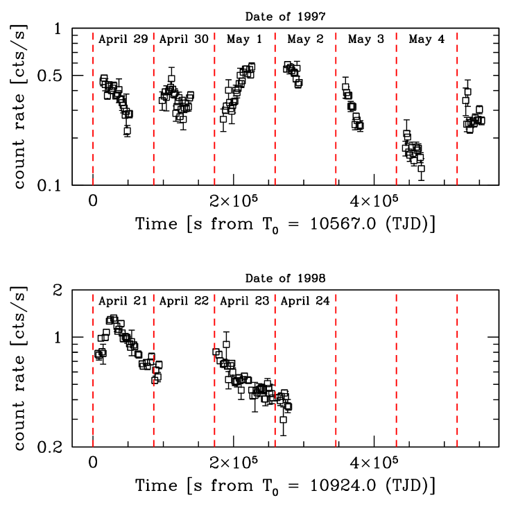
Mkn 421 has been observed by BeppoSAX in the springs of 1997 and 1998. For reference, the BeppoSAX light curves for the 4–6 keV band are reported in Fig. 1. Most of the forthcoming analysis is focused on the spectral variability observed during the flare of 1998 April 21^st, clearly visible in the bottom panel. The journal of observations is given in Table 1 of Paper I.

Figure 1.— Light curves for the 1997 (top panel) and 1998 (bottom panel) campaigns, for the 4–6 keV MECS band. The binning time is 1500 s. The reference time TJD=10567.0 corresponds to 1997–April–29:00:00 UT, and TJD=10924.0 corresponds to 1998–April–21:00:00 UT.

4. Spectral Analysis

In order to unveil the spectral variability during and after the flare, i.e. perform a time resolved spectral analysis, we subdivided the whole dataset in sub–intervals corresponding to single BeppoSAX orbits (42 for the 1997 dataset, 16 on 1998 April 21^st, 19 on 1998 April 23^rd) or a grouping of them sufficient to reach the same statistics (these are reported in Table 1, together with the median time [UTC] of each sub–interval).

LECS and MECS spectra have been accumulated as described in Paper I. LECS data have been considered only in the range 0.12–3 keV due to calibration problems (a spurious hardening) at higher energies (Guainazzi 1997, private comm.)

The nominal full resolution spectra (i.e. channels #11–285 for 0.1–3 keV in the LECS, and #36–220 for 1.6–10 keV in the MECS) have been then rebinned using the grouping templates available at BeppoSAX–SDC The background has been evaluated from the blank fields provided by the BeppoSAX–SDC, using an extraction region similar in size and position to the source extraction region. The Nov. 1998 release of public calibration files, matrices and effective areas was used.

For the PDS spectra we applied the improved screening, implementing the temperature and energy dependence of the pulse rise time (so–called PSA correction method).

Due to a slight mis–match in the cross–calibration among the different detectors, it has been necessary to include in the fitting models multiplicative factors of the normalization (LECS/MECS and PDS/MECS ratios). The correct absolute flux normalization is provided by the MECS (the agreement between MECS units is within the 2–3% limit of the systematics). The expected value of these constant factors is now well known and does not constitute a major/additional source of uncertainty: according to Fiore, Guainazzi & Grandi (cookbook, 1999) the acceptable range for LECS/MECS is 0.7–1.0, with some dependence on the source position in the detectors, while the PDS/MECS ratio can be constrained between 0.77 and 0.95. The latter parameter is indeed crucial in sources like Mkn 421 where there is a significant possibility that a different component arises in the PDS range, whose recognition critically depends on the capability/sensitivity to reject the hypothesis that the PDS counts can be accounted for by the extrapolation of the LECS–MECS spectrum (see Section 4.3.3).

Table 1LECS and MECS Curved Model Spectral Fit: 1997 and 1998

Orbits	Median Obs. Time	spectral indices				$E_{\rm B}$	$E_{\rm peak}$	fluxes			$\chi^{2}_{\nu}$
	UTC	0.5 keV	1 keV	5 keV	10 keV	(keV)	(keV)	0.2-1	2-10	0.1-10
1997 April 29th to May 5th
1–3	1997/04/29:06:08	0.91${}^{+0.04}_{-0.04}$	1.19${}^{+0.05}_{-0.04}$	1.83${}^{+0.05}_{-0.05}$	1.99${}^{+0.13}_{-0.10}$	1.27${}^{+1.15}_{-0.62}$	0.62${}^{+0.05}_{-0.05}$	2.09	1.01	04.68	1.24
4–7	1997/04/29:11:43	1.00${}^{+0.03}_{-0.03}$	1.28${}^{+0.04}_{-0.03}$	1.93${}^{+0.05}_{-0.05}$	2.09${}^{+0.11}_{-0.09}$	1.34${}^{+0.96}_{-0.55}$	0.49${}^{+0.04}_{-0.05}$	1.89	0.75	04.07	1.03
8–10	1997/04/30:05:01	0.94${}^{+0.05}_{-0.06}$	1.24${}^{+0.08}_{-0.06}$	1.91${}^{+0.07}_{-0.06}$	2.08${}^{+0.20}_{-0.13}$	1.26${}^{+1.95}_{-0.79}$	0.57${}^{+0.07}_{-0.08}$	2.15	0.92	04.65	0.95
11–12	1997/04/30:08:37	1.01${}^{+0.04}_{-0.04}$	1.24${}^{+0.05}_{-0.04}$	1.91${}^{+0.07}_{-0.06}$	2.11${}^{+0.21}_{-0.14}$	1.99${}^{+2.65}_{-1.08}$	0.48${}^{+0.07}_{-0.11}$	1.96	0.83	04.29	0.94
13–15	1997/04/30:12:36	0.95${}^{+0.03}_{-0.03}$	1.26${}^{+0.04}_{-0.04}$	1.95${}^{+0.05}_{-0.05}$	2.13${}^{+0.12}_{-0.09}$	1.25${}^{+0.90}_{-0.53}$	0.55${}^{+0.04}_{-0.04}$	1.92	0.78	04.14	0.91
16–18	1997/05/01:05:08	1.03${}^{+0.05}_{-0.05}$	1.35${}^{+0.07}_{-0.07}$	1.84${}^{+0.07}_{-0.06}$	1.94${}^{+0.13}_{-0.09}$	0.57${}^{+0.91}_{-0.42}$	0.46${}^{+0.05}_{-0.07}$	1.99	0.76	04.20	1.14
19–20	1997/05/01:08:43	1.00${}^{+0.04}_{-0.04}$	1.25${}^{+0.05}_{-0.05}$	1.78${}^{+0.06}_{-0.05}$	1.91${}^{+0.14}_{-0.10}$	1.14${}^{+1.51}_{-0.66}$	0.49${}^{+0.06}_{-0.08}$	2.00	0.89	04.42	1.31
21–23	1997/05/01:12:39	0.92${}^{+0.03}_{-0.03}$	1.20${}^{+0.04}_{-0.03}$	1.86${}^{+0.04}_{-0.04}$	2.04${}^{+0.11}_{-0.08}$	1.44${}^{+0.98}_{-0.58}$	0.61${}^{+0.04}_{-0.04}$	2.60	1.22	05.79	1.21
24–25	1997/05/02:05:36	0.93${}^{+0.04}_{-0.04}$	1.18${}^{+0.05}_{-0.04}$	1.83${}^{+0.06}_{-0.05}$	2.00${}^{+0.15}_{-0.11}$	1.57${}^{+1.64}_{-0.80}$	0.61${}^{+0.06}_{-0.07}$	2.74	1.34	06.20	0.77
26–27	1997/05/02:08:35	0.93${}^{+0.05}_{-0.05}$	1.24${}^{+0.06}_{-0.05}$	1.88${}^{+0.06}_{-0.06}$	2.03${}^{+0.15}_{-0.10}$	1.08${}^{+1.27}_{-0.60}$	0.58${}^{+0.06}_{-0.06}$	2.56	1.12	06.20	1.03
28–30	1997/05/03:05:21	1.07${}^{+0.05}_{-0.05}$	1.30${}^{+0.07}_{-0.05}$	1.88${}^{+0.07}_{-0.07}$	2.05${}^{+0.22}_{-0.14}$	1.63${}^{+3.04}_{-1.05}$	0.37${}^{+0.09}_{-0.19}$	2.01	0.78	04.35	1.13
31–32	1997/05/03:08:38	1.05${}^{+0.06}_{-0.06}$	1.28${}^{+0.06}_{-0.05}$	2.13${}^{+0.10}_{-0.09}$	2.49${}^{+0.39}_{-0.24}$	3.50${}^{+6.97}_{-2.05}$	0.39${}^{+0.12}_{-0.19}$	1.65	0.62	03.63	0.79
33–34	1997/05/04:04:22	1.11${}^{+0.07}_{-0.07}$	1.47${}^{+0.13}_{-0.10}$	2.15${}^{+0.15}_{-0.12}$	2.30${}^{+0.37}_{-0.20}$	0.91${}^{+2.84}_{-0.75}$	0.39${}^{+0.07}_{-0.20}$	1.59	0.42	03.16	1.27
35–37	1997/05/04:07:55	1.21${}^{+0.05}_{-0.05}$	1.49${}^{+0.08}_{-0.06}$	2.14${}^{+0.10}_{-0.08}$	2.31${}^{+0.25}_{-0.16}$	1.38${}^{+2.42}_{-0.88}$	0.23${}^{+0.11}_{-0.22}$	1.60	0.40	03.25	0.92
38–40	1997/05/05:05:22	1.10${}^{+0.04}_{-0.04}$	1.43${}^{+0.07}_{-0.06}$	2.01${}^{+0.07}_{-0.07}$	2.13${}^{+0.15}_{-0.11}$	0.74${}^{+1.01}_{-0.47}$	0.39${}^{+0.05}_{-0.09}$	2.04	0.62	04.16	1.07
41–42	1997/05/05:08:46	1.10${}^{+0.06}_{-0.06}$	1.35${}^{+0.08}_{-0.06}$	1.98${}^{+0.10}_{-0.08}$	2.15${}^{+0.29}_{-0.16}$	1.61${}^{+3.73}_{-1.08}$	0.33${}^{+0.10}_{-0.24}$	1.88	0.65	04.00	0.62
1998 April 21st
1–2	1998/04/21:02:55	0.83${}^{+0.05}_{-0.06}$	1.10${}^{+0.07}_{-0.06}$	1.64${}^{+0.06}_{-0.06}$	1.68${}^{+0.09}_{-0.07}$	1.19${}^{+0.47}_{-0.34}$	0.80${}^{+0.10}_{-0.08}$	5.10	3.00	11.96	0.91
3	1998/04/21:05:07	0.87${}^{+0.05}_{-0.05}$	1.02${}^{+0.04}_{-0.04}$	1.65${}^{+0.08}_{-0.07}$	1.74${}^{+0.15}_{-0.10}$	1.82${}^{+0.74}_{-0.49}$	0.92${}^{+0.12}_{-0.10}$	5.34	3.46	13.08	0.97
4	198/04/21:06:40	0.78${}^{+0.04}_{-0.04}$	0.95${}^{+0.03}_{-0.03}$	1.64${}^{+0.06}_{-0.06}$	1.73${}^{+0.11}_{-0.09}$	1.85${}^{+0.51}_{-0.38}$	1.13${}^{+0.11}_{-0.10}$	5.96	4.41	15.22	1.02
5	1998/04/21:08:19	0.81${}^{+0.04}_{-0.04}$	0.96${}^{+0.03}_{-0.03}$	1.58${}^{+0.06}_{-0.05}$	1.66${}^{+0.11}_{-0.08}$	1.82${}^{+0.64}_{-0.44}$	1.09${}^{+0.12}_{-0.10}$	5.77	4.22	14.63	0.86
6	1998/04/21:09:56	0.80${}^{+0.04}_{-0.04}$	1.03${}^{+0.05}_{-0.04}$	1.50${}^{+0.05}_{-0.05}$	1.53${}^{+0.07}_{-0.06}$	1.16${}^{+0.40}_{-0.30}$	0.91${}^{+0.10}_{-0.09}$	5.35	3.76	13.24	1.17
7	1998/04/21:11:32	0.79${}^{+0.04}_{-0.04}$	1.00${}^{+0.05}_{-0.04}$	1.53${}^{+0.06}_{-0.05}$	1.57${}^{+0.08}_{-0.07}$	1.36${}^{+0.46}_{-0.33}$	0.98${}^{+0.11}_{-0.10}$	5.05	3.62	12.64	0.85
8–9	1998/04/21:13:57	0.85${}^{+0.03}_{-0.03}$	1.05${}^{+0.04}_{-0.03}$	1.50${}^{+0.04}_{-0.04}$	1.54${}^{+0.06}_{-0.05}$	1.26${}^{+0.35}_{-0.27}$	0.85${}^{+0.07}_{-0.06}$	4.62	3.10	11.35	1.38
10–12	1998/04/21:17:57	0.87${}^{+0.02}_{-0.02}$	1.05${}^{+0.03}_{-0.02}$	1.54${}^{+0.04}_{-0.03}$	1.58${}^{+0.05}_{-0.04}$	1.40${}^{+0.30}_{-0.24}$	0.85${}^{+0.06}_{-0.05}$	3.99	2.63	09.76	0.89
13–16	1998/04/21:23:35	0.91${}^{+0.03}_{-0.03}$	1.06${}^{+0.03}_{-0.02}$	1.61${}^{+0.05}_{-0.05}$	1.67${}^{+0.08}_{-0.07}$	1.67${}^{+0.48}_{-0.36}$	0.79${}^{+0.07}_{-0.07}$	3.61	2.23	08.73	0.99
1998 April 23rd
1–5	1998/04/23:03:49	0.93${}^{+0.02}_{-0.03}$	1.10${}^{+0.03}_{-0.02}$	1.67${}^{+0.04}_{-0.04}$	1.74${}^{+0.07}_{-0.05}$	1.59${}^{+0.37}_{-0.29}$	0.71${}^{+0.05}_{-0.05}$	4.15	2.32	09.74	1.11
6–11	1998/04/23:12:31	0.95${}^{+0.02}_{-0.02}$	1.17${}^{+0.02}_{-0.02}$	1.78${}^{+0.03}_{-0.03}$	1.84${}^{+0.05}_{-0.04}$	1.47${}^{+0.21}_{-0.18}$	0.60${}^{+0.03}_{-0.04}$	3.73	1.78	08.42	1.27
12–19	1998/04/23:23:39	1.03${}^{+0.02}_{-0.02}$	1.19${}^{+0.02}_{-0.02}$	1.79${}^{+0.04}_{-0.04}$	1.85${}^{+0.06}_{-0.05}$	1.68${}^{+0.32}_{-0.26}$	0.38${}^{+0.09}_{-0.23}$	3.25	1.47	07.30	1.16

Table 2Summary of Power Law models Results

		1997					1998
Model		NH	$\chi^{2}$	$\chi^{2}_{\nu}$	d.o.f.		NH	$\chi^{2}$	$\chi^{2}_{\nu}$	d.o.f.
single P.L.		Galactic	11903.1	12.609	944		Galactic	11245.0	15.883	708
single P.L.		$3.78\pm 0.18$	03012.7	03.246	928		$3.22\pm 0.14$	03413.2	04.905	696
broken P.L.		Galactic	01162.6	01.275	912		Galactic	00997.6	01.458	684
broken P.L.		$2.23\pm 0.46$	01083.2	01.209	896		$2.05\pm 0.19$	00866.6	01.289	672
curved		Galactic	00935.7	01.026	912		Galactic	00721.1	01.054	684
curved		$1.73\pm 0.12$	00917.8	01.024	896		$1.70\pm 0.12$	00705.2	01.049	672

Figure 2.— Data/Model ratios for different spectral models applied to the 1998 data. Top to bottom: single power law with (a) Galactic and (b) free absorbing column, broken power law with (c) Galactic and (d) free absorbing column, curved model, with (e) Galactic and (f) free absorbing column. The corresponding values of $\chi^{2}$ are reported in Table 2.

4.1. Single and Broken Power Laws

We do not discuss in detail any power law spectral models. For each LECS$+$MECS spectrum we fit the data with the single and the broken power law models, both with free and fixed absorbing column density.

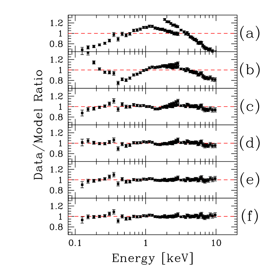
Here we just show that they are an inadequate description of the downward curved spectra. To illustrate the discrepancy, we took the data/model ratio for the best fit continuum model, for each of the individual LECS$+$MECS spectra (16 for 1997, 12 for 1998), and we summed all of them, propagating the errors accordingly. The results are shown in Figure 2 for the 1998 data only, while in Table 2 we report the total $\chi^{2}$ value for each trial model, together with the (simple) average value of N_H for fits with free absorption.

Neither the single nor the broken power laws provide an adequate representation of the data, not even when the value of the absorbing column density is left free to vary –a common workaround used when the spectrum shows either a soft excess or a marked steepening toward higher energies (e.g. Takahashi et al. takahashi96, 1996).

Indeed the description of the curvature by means of soft X–ray absorption is not only un–physical, but it hinders the possibility of extracting all the information from the data, by leaving as meaningful parameter only the higher energy spectral index and accounting for all the other effects by N_H. Furthermore this yields spectral indices that are only rough estimates, as it is clear that the best fit single power law does not describe the observed data in any (even narrow) energy range (see Figure 2a,b). Finally, in the case of Mkn 421 there is no reason to postulate any intrinsic absorbing component responsible for the observed spectral curvature (see also §4.3.2).

4.2. The Curved Model

Motivated by the failure of the simplest power law models, we developed a spectral model which is intrinsically curved, with the aim of extracting all the information contained in the data, and in particular estimate the position of the peak of the synchrotron component, one of the crucial quantities in blazars modeling.

A spectral model providing an improved description of the continuum shape also allows a more sensitive study of discrete spectral features such as absorption edges, whose presence has been long searched in the soft X–ray blazars spectra (e.g. Canizares & Kruper canizares84, 1984; Sambruna et al. sambruna_1426, 1997; Sambruna & Mushotzky sambruna_0548, 1998).

We started from the following general description of a continuously curved shape (see e.g. Inoue & Takahara inoue_takahara96, 1996, Tavecchio, Maraschi & Ghisellini tavecchio_etal98, 1998):

$$F(E)\;=\;K\;E^{-\alpha_{-\infty}}\;\left(1+\left(\frac{E}{E_{\rm B}}\right)^{f}\right)^{\frac{\alpha_{-\infty}-\alpha_{+\infty}}{f}}$$ (1)

where $\alpha_{-\infty}$ and $\alpha_{+\infty}$ are the asymptotic values of spectral indices for $E\ll E_{\mathrm{B}}$ and $E\gg E_{\mathrm{B}}$ respectively, while $E_{\mathrm{B}}$ and $f$ determine the scale length of the curvature.

We re–expressed this function in terms of the spectral indices at finite values of $E$, which characterize the local shape of the spectrum, instead of the asymptotic ones, which do not have any direct reference to the observed portion of the spectrum.

The spectral model is then expressed in a form such that the available parameters are $(E_{1},\alpha_{1},E_{2},\alpha_{2},E_{\mathrm{B}},f)$ instead of ($\alpha_{-\infty}$, $\alpha_{+\infty}$, $E_{\mathrm{B}}$, $f$) (for more details see Appendix B). As we have two extra parameters, for a meaningful use of this spectral description we have to fix one for each of the pairs $(E_{1},\alpha_{1})$ and $(E_{2},\alpha_{2})$. Eventually this degeneracy turns out to be a powerful property of this model, because it allows us to derive the spectral index at selected energies (setting $E_{\mathrm{i}}$ at the preferred values), or even more interestingly to estimate the energy at which a certain spectral index is obtained (setting $\alpha_{\mathrm{i}}$ at the desired value). The most relevant example of this latter possibility is the determination of the position of the peak (as seen in $\nu F_{\nu}$ representation) of the synchrotron component $E_{\mathrm{peak}}$ –if it falls within the observed energy band– and the estimate of the associated error. This can be obtained by setting one spectral index, i.e. $\alpha_{1}=1$, and leaving the corresponding energy $E_{1}$ free to vary in the fit: the best fit value of $E(\alpha=1)$ gives $E_{\mathrm{peak}}$.

Figure 3.— Inferred BeppoSAX $\nu F_{\nu}$ spectra of Mkn 421 in 1998. The plotted spectra correspond to the orbit groupings 1$+$2, 4, 8$+$9 of April 21^st, and 12–19 of April 23^rd (see Table 1). For comparison we also plotted in light grey color the spectrum of the previous box.

4.3. Results

Most of the spectral analysis with the curved model has been performed by keeping the absorbing column fixed to the Galactic value, to remove the degeneracy between the effects of a variable absorption and intrinsic spectral curvature. We will briefly comment on the fits with a variable absorbing column in the next section.

In order to determine the values for the really interesting parameters, we tried a set of values for the parameter $f$, ranging from 0.5 to 3 (with a step of 0.5). All the other parameters were left free to vary during these step–fits. We then selected the value of $f$ yielding the minimum total $\chi^{2}$. The best fit value for 1997 is $f=1$, while for 1998 $f=2$, as expected from the stronger curvature of the spectra. In Table 1 we report the spectral parameters, together with the 0.2–1, 2–10 and 0.1–10 keV fluxes (de–reddened) and $\chi^{2}$ values, for each of the time sliced spectra. The global Data/Model ratio is shown in Figure 2e, and the total $\chi^{2}$ is reported in Table 2. The curved model is strongly preferred also from the purely statistical standpoint: in fact the model with Galactic N_H has a significantly better $\chi^{2}$ than the broken power law with free N_H, although it has one less adjustable parameter (i.e. one more degree of freedom).

Each spectrum has been fitted a few times in order to derive spectral indices at several energies (0.5, 1, 5, 10 keV), and also E_peak. For consistency we checked each time that not only the value of the $\chi^{2}$ remained the same, but also all the other untouched parameters took the same value and confidence intervals. The fits are indeed very robust in this sense.

The main new result is that we were able to determine the energy of the peak of the synchrotron component, and to assign an error to it. This has been possible with reasonable accuracy for both 1997 and 1998 spectra, with a couple of cases yielding only an upper limit for the peak energy.

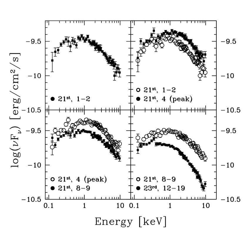
An example of the remarkable spectral evolution during the 1998 flare is shown by the deconvolved spectra in Figure 3, which also illustrates the strong convexity of the spectrum and the well defined peak.

In 1997 the source was in a lower brightness state, with an average X–ray spectrum softer (at all energies $\Delta\alpha_{97\longrightarrow 98}\simeq 0.4$), and a peak energy 0.5 keV lower.

Figure 4.— (a) spectral index at 5 keV and (b) synchrotron peak energy plotted versus the de–absorbed 0.1–10 keV flux, both for 1997 and 1998 datasets. The dashed line across the diagram (b) represents the best fitting power law, with a slope $\epsilon=0.55$.

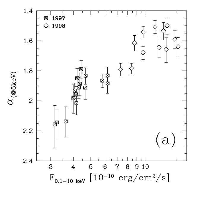
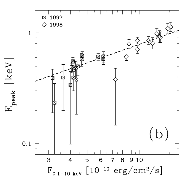
More globally, the analysis shows that there is a clear relation between the flux variability and the spectral parameters, both in 1998 and, albeit less strikingly, in 1997. Particularly important is the correlation between changes in the brightness (even the small ones) and shifts of the peak position, as the latter carries direct information on the source physical properties. In Figure 4a,b, $\alpha$ at 5 keV and E_peak for 1997 and 1998 are plotted versus the 0.1–10 keV flux. The source reveals a coherent spectral behavior between 1997 and 1998 and through a large flux variability (a factor 5 in the 0.1–10 keV band). Both the peak energies and the spectral indices show a tight relation with flux, the latter being described by E${}_{\mathrm{peak}}\propto\mathrm{F}^{\epsilon}$, with $\epsilon=0.55\pm 0.05$.

4.3.1 Hard Lag in 1998 spectra

One further important finding of the time resolved spectral study is the signature of the hard lag which strengthens what already inferred from the timing analysis (see Paper I). In fact the local spectral slope at different energies indicates that the flare starts in soft X–rays and then extends to higher energies.

Figure 5.— Top to bottom: the energy of the peak of the synchrotron component, and the photon spectral indices at 5 and at 1 keV versus time (left column) and de–absorbed 0.1–10 keV flux (right column). The solid black symbols represent the behavior before the top of the flare, while empty dots represent the spectral evolution during the decay. The data points are connected to show the time sequence. A shift of the synchrotron peak and a delay in the response of the spectrum at 5 keV can be clearly seen.

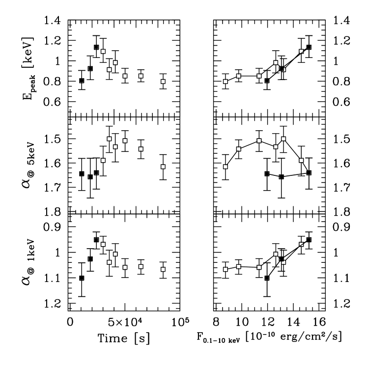
A blow up of the 1998 flare interval is shown in Figure 5: spectral indices at 1 and 5 keV, and E_peak are plotted versus time in the left hand plots, and versus flux in the right hand ones. The synchrotron peak shifts toward higher energies during the rise and then decreases as soon as the flare is over. The spectral index at 1 keV reflects exactly the same behavior, as expected being computed at the energy around which the peak is moving (and in fact it moves in a narrow range around $\alpha=1$). On the contrary, the spectral shape at 5 keV does not vary until a few ks after the peak, and only then –while the flux is decaying and the peak is already receding– there is a response with a significant hardening of the spectrum. The right side diagrams illustrate this behavior directly in terms of flux: the evolution of the peak energy and the 1 keV spectral shape follow closely that of the flare, while at 5 keV the spectrum does not change shape until after the peak.

Thus the spectral evolution at higher energies develops during the decay phase of the flare, tracing a loop in the $\alpha$ vs. Flux diagram, with a significant hardening of the spectrum. Due to the presence of the hard lag, the loop is traced in the opposite way with respect the evolution that is commonly observed during flares in HBL, that is a spectral hardening during the rise of the outburst, followed by a softening during the decay (see however Sembay et al. sembay_2155, 1993, Catanese & Sambruna catanese_sambruna_00, 2000).

This behavior –usually accompanied by a soft lag– produces a clockwise loop in $\alpha$ vs. Flux.

4.3.2 Absorption Features: N_H and edges

We also fit the 1997 and 1998 spectra with the curved spectral model leaving the N_H free to vary. The only constraint that we imposed is on the exponent $f$, which is set at the best fit values of $f=1$ and $f=2$ for 1997 and 1998, respectively. The improvement of the global fit is not statistically significant. The average best fit absorbing column is indeed very close to and consistent with the Galactic one, leading us to conclude that there is no requirement whatsoever for an additional absorbing column to model the data.

We searched for the presence of absorption edges at low energies (E $\lesssim$ 1 keV), both in 1997 and 1998 data. We added to the curved continuum an absorption edge, with a first guess fit at E$\simeq 0.4-0.5$ keV, as even in the case of the best curved model with free N_H there are residues around this energy (see Figure 2f). The most delicate issue is the calibration problem related with the instrumental Carbon absorption edge at 0.29 keV. Even the smallest uncertainties ($\sim 1-2$%) in the knowledge of the instrument response around this energy can induce significant spurious features, typically at slightly higher energy (see Fossati & Haardt fg_fh_lecs, 1997).

There is not convincing evidence for discrete absorption features. In 5/28 cases the fit routine has not found an edge, while there are indeed a few spectra (8/28) in which the fit definitely put the edge at 0.27–0.30 keV, to account for systematic deviation due to calibration uncertainties. There are then 15/28 cases where the edge energy is around 0.4–0.6 keV, but again only in a handful of cases the best fit energy E_edge is significantly different from 0.29 keV.

Summarizing, there are only three individual spectra (out of 28) for which the inclusion of the edge is formally statistically significant ($>$ 95%), according to the F–test. These three cases do not stand out in the sample for any other property, such as brightness or curvature of the continuum. Best fit energies and optical depths are typically E${}_{\mathrm{edge}}\simeq 500^{+50}_{-100}$ eV, and $\tau\simeq 0.4^{+0.3-0.6}_{-0.2}$. However, considering that the sample comprises 28 spectra, with the significance threshold set at 95%, three positive detections can not be regarded as a compelling evidence for the presence of absorption edges.

4.3.3 PDS data

Covering the range above $\simeq 12$ keV, the PDS instrument could detect the IC component, which might start to dominate the emission in this band. It has always proven to be very difficult to detect/constrain this component, although it is expected to have a very hard spectrum, that should make it easier to disentangle from the very steep tail of the synchrotron component. There are a few objects, the so–called intermediate BL Lacs, in which the cross–over between synchrotron and IC occurs in the 0.1–10 keV band, for which it has then been possible to clearly detect the hard IC power law, with typical $\alpha\simeq 0.3-0.7$ (e.g. Tagliaferri et al. tagliaferri_on231, 2000 for ON 231; Giommi et al. giommi_0716, 1999 for S5 0716$+$714; Sambruna et al. sambruna_bllac_99, 1999 for BL Lac). The good sensitivity of the PDS yielded a convincing evidence of IC emission in the case of PKS 2155$-$304 (Giommi et al. giommi_2155, 1998). The preliminary analysis of the Mkn 421 1997 data (Fossati et al. 1998b, ) suggested the presence of a hard component. We therefore focused on the search for the IC component for both of 1997 and 1998 PDS datasets.

For 1998, when the source was brighter, we accumulated PDS spectra according to the same partition of the light curves used for the 0.1–10 keV data. In most of the individual spectra there is a significant ($\geq$3-$\sigma$) detection only up to 40 keV. The light curve for the 12–26 keV band is shown in Figure 3 of Paper I.

We then restricted the analysis to only one spectrum for 1997, integrating over the whole campaign, and two for 1998, one for April 21^st, and one for April 23^rd. The integration times are 54.8, 21.1 and 25.2 ks respectively (see Paper I). We grouped the data in 6 channels spectra with boundaries at 12, 18, 27, 40, 60, 90 and 130 keV.

In the 1997 spectrum there is a positive detection up to 90 keV. For April 21^st –corresponding to the synchrotron flare– there is a strong signal up to 60 keV, while, surprisingly, in the April 23^rd spectrum there is a $\gtrsim$3-$\sigma$ detection in each individual bin up to 130 keV. From 12 to 40 keV the April 21^st count rates are significantly higher than those of April 23^rd, but while the former continue to steeply decrease with increasing energy, the latter flatten above 40 keV, with a cross over in the 40–60 keV bin. As the integration times for these two spectra are similar (and in fact statistical uncertainties on the count rate are of the same order), this cannot account for this difference.

The results of single power law fits are reported in Table 3: clearly the April 23^rd spectrum is significantly harder. Moreover, the spectral indices for the first two cases are consistent with those derived from the LECS and MECS datasets and the general picture of a continuously steepening spectrum, while this does not hold for the third case.

While this is already interesting, there is one additional, somehow unexpected, finding: apparently the April 23^rd harder spectrum cannot be simply interpreted as the detection of the IC component when the synchrotron tail recedes. In fact a hard power law at this flux level –if present– would have been detected also on April 21^st, while the count rates in the higher energy bins for April 21^st set a tight upper limit. This behavior might be ascribed to either a different independent origin or a delayed response of the IC component with respect to the synchrotron one (indeed some evidence of a possible delayed decay of the PDS with respect to the MECS emission can be seen in the light curves).

Table 3PDS single power law fits: 1997 and 1998

			Count rates
Dataset	Band	Exposure	12–40 keV	40–90 keV	$\alpha$	F1keV	$\chi^{2}$	d.o.f.
		(ks)	(cts/s)	(cts/s)		($\mu$Jy)
1997	12–90 keV	54.8	0.177 $\pm$ 0.021	0.045 $\pm$ 0.019	2.17${}^{+0.48}_{-0.41}$	1.52	2.96	3
1998 April 21st	12–90 keV	21.1	0.698 $\pm$ 0.028	0.039 $\pm$ 0.023	2.23${}^{+0.14}_{-0.13}$	5.76	1.76	3
1998 April 23rd	12–90 keV	25.2	0.293 $\pm$ 0.025	0.081 $\pm$ 0.021	1.35${}^{+0.26}_{-0.24}$	1.35	6.95	4
	12–130 keV	$\cdots$	$\cdots$	$\cdots$	1.54${}^{+0.28}_{-0.25}$	1.54	2.95	3

Table 4High energy component constraints from MECS$+$PDS spectral fits

	High Energy Component Flux			Synchrotron Flux
Dataset	12–40 keV	40–100 keV		12–40 keV	40–100 keV	$\chi^{2}$	d.o.f.
1997	$<$ 11.0${}^{+2.1}_{-2.6}$	$<$ 12.8${}^{+3.7}_{-2.1}$		07.8	0.2	17.92	15
1998 April 21st	$<$ 13.0${}^{+2.1}_{-2.6}$	$<$ 14.9${}^{+2.1}_{-2.6}$		78.4	8.6	28.71	30
1998 April 23rd	$<$ 13.6${}^{+3.3}_{-3.1}$	$<$ 15.8${}^{+3.8}_{-3.6}$		24.0	1.2	$\cdots$	$\cdots$
1998 April 21st $+$ 23rd	$<$ 10.1${}^{+3.1}_{-2.9}$	$<$ 11.8${}^{+3.5}_{-3.4}$		78.4 / 24.0	8.6 / 1.2	34.79	31

Finally we tried to quantify the presence of the IC power law in the three datasets by fitting MECS and PDS data together. We proceeded in the following way:

• We accumulated LECS and MECS spectra over the same intervals of the PDS ones, i.e. one cumulative spectrum for each day of 1998, and one for the whole 1997.

• We fit the LECS$+$MECS spectra in order to constrain the average synchrotron spectrum.

• We then fixed all the parameters of the curved model to the LECS$+$MECS best fit values, and added to the model a hard power law component with fixed spectral index (we tried the values $\alpha_{\mathrm{IC}}=0.4,0.5,0.6,0.7$). We also added an exponential cut–off to the synchrotron component setting its two parameters, i.e. cut–off and e–folding energies, to 10 and 40 times the best fit value of E_peak.

• We used this partially constrained model to fit the MECS (above E$\geq 5$ keV) and PDS spectra. The two 1998 datasets have been fit jointly with PDS/MECS intercalibration factor free to vary, but set to be the same for both, and of course independent normalization.

The results are reported in Table 4, for the $\alpha_{\mathrm{IC}}=0.5$ case (the values relative to the other $\alpha_{\mathrm{IC}}$ are not significantly different). The best fit PDS/MECS normalization ratio is 0.88.

There seems to be a significant change in the flux level of the expected IC component between 1998 April 21^st and 23^rd. The best fit value for the normalization for the first day is zero, while for the second day a non–zero IC flux is definitely required. In order to test the likelihood of the apparent variation, we fit the data constraining the normalization to be the same for the two datasets (third case in Table 4) and the F–test probability to obtain by chance the observed change in $\chi^{2}$ is $\sim$ 0.01 ($\triangle\chi^{2}=6.08$, d.o.f. from 30 to 31).

The basic result for 1997 is that the IC component is definitely detected. Its brightness level is comparable with the average of 1998, while the synchrotron component shows a significant variation.

It should be noted that the synchrotron fluxes reported in Table 4 are not the best reference because at those energies, well above the synchrotron peak, the spectrum is very steep and even the smallest shift of the peak energy translates in a big change in the flux. Nevertheless even when considering the energy range 0.1–10 keV, which includes the synchrotron peak, the variation between 1997 and 1998 is of the order of a factor of 2–3 (e.g. Figure 5). The sampling of the 1997 light curve is not good enough to enable us to investigate any possible variation of the PDS spectrum with the source brightness.

5. Discussion

Before focusing on the modeling of the temporal and spectral behavior illustrated in this paper and in Paper I, let us consider a few issues which we consider of particular relevance for the interpretation of the origin of blazar variability.

5.1. Spectral Variability, Synchrotron Peak and IC component

Soft and hard X–ray bands show a different behavior. This might be attributed to the contribution from both the synchrotron and inverse Compton components at these energies. As electrons emitting X–rays through the two processes would have different energies, the two components are not expected to vary on the same timescales and in phase. Indeed on one hand the constraints provided by the analysis of the PDS data suggest that the synchrotron component constitutes the dominant contribution to the flux in the 12–26 keV band on 1998 April 21^st (during the flare) with a light curve somewhat different from that of the softer synchrotron X–rays. On the other hand, the evidence supporting the possibility of a substantial variation in the IC component during the 1998 observations is extremely interesting. We can rule out the possibility that the flux level of the hard component is approximately constant between the two observations of 1998 (with a 99% confidence), and thus that its detectability only depends on the the brightness level of the tail of the synchrotron emission.

5.2. The Flaring + Steady Components Hypothesis

A further interesting issue raised in Paper I in connection with the temporal analysis is the presence and role of quasi–stationary emission. Our results support the view that the short–timescale, large–amplitude variability events could be attributed to the development of new individual flaring components, giving rise to a spectrum out–shining a more slowly variable contribution.

Indeed there is growing evidence that the overall blazar emission comprises a component that is (possibly) changing only on long timescales and that does not take part in the flare events (see for instance Mkn 501, Pian et al. pian_mkn501_98, 1998, and Pian et al. pian_3c279, 1999 for the case of the UV variability of 3C 279).

The deconvolution of the SED into different contributions would allow the study of the evolution of the flaring component possibly clarifying the nature of the dissipation events occurring in relativistic jets –in particular the particle acceleration mechanism– and the modality and temporal characteristics of the initial release of plasma and energy through these collimated structures.

The deconvolution is however still difficult to achieve with the available temporal and spectral information. In paper I we discussed the results of our attempt to measure directly the relative contributions of what we identify as steady and flaring components (parameter ${\cal R}$), from the characteristics of the flare decay. The result is very interesting, although it does not provide a useful handle on the evolving spectral properties of the flare itself. A more feasible approach is to assume specific forms of the flare evolution and test them against the data. One of the simplest working hypothesis is to assume that the flare evolution can be reproduced by the time dependent flux and energy shifts of a peaked spectral component with fixed spectral shape (e.g. Krawczynski et al. krawczynski_mkn501_2000, 2000). In this context it is relevant to remind that the maximum of the synchrotron emission corresponds to the energy at which most of the energy in particles is located. Its value and temporal behavior thus trace the evolution of the bulk of the energy deposition into particles by the dissipation mechanism.

It is therefore possible that the variability characteristics (both temporal and spectral) might chiefly depend on the (particles/photons) energy relative to the synchrotron peak. In particular, the results on T_short (Paper I) can be either related to the dominance of the light crossing time over the cooling timescales, or alternatively to the different position of the sampled energies with respect to the synchrotron peak as above the peak the timescales are shorter. In any case the fact that timescales are similar at the different energies possibly indicates the evolution of a (observed) fixed–shape flaring component.

5.3. Sign of the lag

One of the main new results of the temporal analysis presented in Paper I is the significant detection of a hard lag, opposite to the behavior commonly detected in HBL. Interestingly, a recent study by Zhang et al. (zhang_2155, 1999) on the source PKS 2155–304 has shown the presence of an apparent inverse trend between the source brightness level and the duration of the (soft) lag. And intriguingly, the 1998 flare represents the brightest state ever observed from Mkn 421, thus possibly suggesting that an extrapolation of the above phenomenological trend might even account for a hard lag. This possibility is currently under study (Zhang et al., in preparation).

Again the relative contribution of two components might be responsible for this trend. During the most intense events the flaring component would completely dominate over the quasi–stationary one, progressively shifting to higher energies (hard lag), while in weaker flares the varying component would exceed the steady one only at energies higher than the peak, where the spectrum steepens, producing an observed soft lag behavior.

However, one should also consider that in different brightness states the different observed energies correspond to different positions with respect to E_peak (e.g. comparing the 1997 and 1998 datasets we showed that its value was typically a factor 2 different), requiring a more subtle analysis before deriving inferences on the lag–brightness relationship.

5.4. Physical Interpretation: the signature of particle acceleration

Let us now focus on the interpretation of the two main and robust results of this work, namely the hard lag and the evolution of the synchrotron peak.

The occurrence of the peak at different times for different energies is most likely related to the particle acceleration/heating process. Although models to reproduce the temporal evolution of a spectral distribution have been developed (e.g. Chiaberge & Ghisellini chiab_gg, 1999, Georganopoulos & Marscher markos_98, 1996; Kirk, Rieger & Mastichiadis kirk_etal_98, 1998), they mostly do not consider the role of particle acceleration (see however Kirk et al. kirk_etal_98, 1998).

In order to account for the above results, we thus introduced a (parametric) acceleration term in the particle kinetic equation within of the time dependent model studied by Chiaberge & Ghisellini (chiab_gg, 1999). In particular, this model takes into account the cooling and escape in the evolution of the particle distribution and the role of delays in the received photons due to the light crossing time of different parts of the emitting region.

The model includes the presence of a quiescent spectrum, which is assumed to be represented by and thus fitted to the broad band spectral distribution observed in 1994 (Macomb et al. macomb95, 1995). To this a flaring component is added and this is constrained by the observed spectral and temporal evolution (the parameters for both the stationary and variable spectra are reported in Table 5). The values of the model parameters are very close to those derived in Maraschi et al. (maraschi_letter, 1999) in a somewhat independent way, i.e. trying only to fulfill the constraints provided by the X–ray and TeV spectra, simultaneous but averaged over the whole flare. On this basis it is very likely that the model discussed here satisfies the TeV constraints, which are however not directly taken into account (the computation of the TeV light curve in this complex model would require to treat the non–locality of the IC process, which is beyond the scope of this paper).

Clearly a parametric prescription does not reproduce a priori a specific acceleration process, but we rather tried to constrain its form from the observed evolution. The main constraints on the form of the acceleration term are the following:

• Particles have to be injected at progressively higher energies on the flare rise timescale to produce the hard lag.

• Globally the range of energies over which the injection occurs has to be narrow, to give rise to a peaked spectral component.

• A quasi–monochromatic injection function for the flux at the highest energies to reach its maximum after that at lower ones (as opposed to e.g. a power law with increasing maximum electron Lorentz factor).

• The emission in the LECS band from the particles which have been accelerated to the highest energies (i.e. those radiating initially in the MECS band) should not exceed that from the lower energy ones, as after the peak no further increase of the (LECS) flux is observed; this in particular requires for the injection to stop after reaching the highest energies.

• The total decay timescale might be dominated by the achromatic crossing time effects, although the initial fading might be determined by different cooling timescales.

Figure 6.— Light curves computed from the model, at the centroid energies of the soft and hard band considered in the data analysis. The vertical axis represents the variations normalized to the flux of the stationary component.

Figure 7.— X–ray spectra at different times, as derived from the model. On each spectrum we marked the position of the synchrotron peak with a symbol.

Table 5Model Parameters

Parameter	Parameter Description	stationary	flaring
$R$	source dimension (cm)	2 $\cdot 10^{16}$	2 $\cdot 10^{16}$
$B$	magnetic field (G)	0.12	0.03
$t_{esc}$	escape timescale (R/c)	6	1.5
$\ell_{\mathrm{inj}}$	compactness injected as particle energy	6 $\cdot 10^{-5}$	3 $\cdot 10^{-4}$
$s$	slope of the injected stationary power law	1.6	$\cdots$
$\gamma_{\mathrm{max}}$	maximum Lorentz factor of the injected stationary power law	3 $\cdot 10^{5}$	$\cdots$
$\gamma_{\mathrm{c,max}}$	maximum Lorentz factor of Gaussian injection for the flaring component	$\cdots$	7 $\cdot 10^{5}$
$\delta$	beaming factor	18	18

The acceleration term has then been described as a Gaussian distribution in energy, centered at a typical particle Lorentz factor $\gamma_{\mathrm{c}}(\mathrm{t})$ and with width $\sigma=0.01\gamma_{\mathrm{c}}(\mathrm{t})$, exponentially evolving with time: $\gamma_{\mathrm{c}}(\mathrm{t})\propto e^{-(\mathrm{t}_{\mathrm{max}}-\mathrm{t})}$, where t_max corresponds to the end of the acceleration phase, when the maximum $\gamma_{\mathrm{c,max}}$ is reached. The injected luminosity is assumed to be constant in time.

The duration of the injection, assumed to correspond to the light crossing time of the emitting region, is such that it mimics the passage of a shock front (i.e. a moving surface passing through the region in the same time interval, see Chiaberge & Ghisellini chiab_gg, 1999).

It should be also noted that, within this scenario, the symmetry between the rise and decay in the soft energy light curve seems to suggest that if the energy where most of the power is released is determined by the balance between the acceleration and cooling rates, at this very same energy the latter timescales are comparable to the light crossing time of the region.

The predictions of the model are shown in Figures 7 and 7, in the form of light curves and spectra at different times, respectively. In particular, in Figure 7 the light curves (normalized over the stationary component) at the two centroid energies of the soft and hard bands considered in the data analysis are reported. The presence of a hard lag is clearly visible as well as the larger variability amplitude at higher frequencies. Also the spectral evolution, reported in Figure 7 in $\nu F_{\nu}$ in the observed energy range, seems to be at least in qualitative agreement with what observed (compare with Fig. 3).

A posteriori it is important to notice that the inclusion of a quasi–stationary component and of high energy emission (from synchrotron self–Compton) are indeed crucial in order to reproduce the retarded spectral variability at energies above a few keV. This constitute a further difference with respect to the discussion of Maraschi et al. (maraschi_letter, 1999), where a simplified description of the time decay was used, based on evidence for an energy dependence of the flare decay timescale (obtained modeling the decay with no baseline).

6. Conclusions

BeppoSAX has observed Mkn 421 in 1997 and 1998. We analyzed and interpreted the combined spectral and temporal evolution in the X–ray range. During these observations the source has shown a large variety of behaviors, both concerning the X–ray band itself and its variability properties with respect to the $\gamma$–ray one, providing us with a great wealth of information, but at the same time revealing a richer than expected phenomenology.

Several important results follow from this work:

• The X–ray and 2 TeV light curves peak simultaneously within one hour, although the halving time in the TeV band seems shorter than those at LECS and MECS energies (see Maraschi et al. maraschi_letter, 1999).

• The detailed comparison of 0.1–1.5 keV and 3.5–10 keV band light curves shows that the higher energy band lags the softer one, with a delay of the order of 2–3 ks. This finding is opposite to what has been commonly observed in HBL X–ray spectra (see Paper I).

• Moreover, extracting LECS$+$MECS spectra for $\lesssim$ 5 ks intervals, we were able to follow in detail the spectral evolution during the flare. For the first time we could quantitatively track the shift of the peak of the synchrotron component moving to higher energy during the rising phase of the flare, and then receding.

• An energy dependence of the shape of the light curve during the flare has been revealed: at low energies the shape is consistent with being symmetric, while at higher energies is clearly asymmetric (faster rise) (see Paper I).

• Evidence has been found for the presence of the IC component, and more importantly for its substantial variability, which is possibly delayed with respect to the synchrotron one.

These findings provide several temporal and spectral constraints on any model. In particular, they seem to reveal the first direct signature of the ongoing particle acceleration mechanism, progressively “pumping” electrons from lower to higher energies. The measure of the delay between the peaks of the light curves at the corresponding emitted frequencies thus provides a tight constraint on the timescale of the acceleration process.

Indeed, within a single emission region scenario, we have been able to reproduce the sign and amount of lag by postulating that particle acceleration follows a simple exponential law in time, stops at the highest particle energies, and lasts for an interval comparable to the light crossing time of the emitting region. If this timescale is intrinsically linked to the typical source size, we indeed expect the observed light curve to be symmetric at the energies where the bulk of power is concentrated and an almost achromatic decay. The same model can account for the spectral evolution (shift of the synchrotron peak) during the flare.

The other very important clue derived from the analysis is the presence of a quasi–stationary contribution to the emission, which seems to be dominated by a highly variable peaked spectrum, possibly maintaining a quasi–rigid shape during flares. The decomposition of the observed spectrum into these two components might allow us to determine the nature and modality of the energy dissipation in relativistic jets.

Appendix A A. A caveat on continuously curved spectral models

The increasing quality of the available X–ray spectral data, both in terms of signal–to–noise ratio and energy resolution, has made necessary to consider more complex fitting models. One of the most interesting continuum feature in the X–ray spectra of blazars is the curvature of the synchrotron component, as good quality data could enable us to estimate the energy of the emission peak. As clearly the traditional single or broken power law models are unsatisfactory, we developed the curved spectral model presented in this paper: a simple analytic expression representing a continuous curvature, two “pivoting” points –useful for analysis purposes– asymptotically joining two power law branches, whose slope is completely determined by the behavior of the function at the pivoting energies.

Another increasingly popular model has been introduced by Giommi et al. (giommi_2155, 1998) (to reproduce BeppoSAX data of PKS 2155$-$304, and then used also for Mkn 421 by Guainazzi et al. guainazzi_mkn421, 1999 and Malizia et al. malizia_mkn421, 1999), but unfortunately this is affected by a problem that can lead to misleading results.

This more generally occurs for all curved continuum models defined as:

$$F(E)\;=\;E^{-\tilde{\alpha}(E)}$$ (A1)

where the function $\alpha(E)$ is suitably defined to smoothly change between two asymptotic values $\alpha_{1}$ and $\alpha_{2}$. The specific choice by Giommi et al. (giommi_2155, 1998) is:

$$\tilde{\alpha}(E)\;=\;f(E)\alpha_{1}+(1-f(E))\alpha_{2}$$ (A2)

with

$$f(E)\;=\;\left(1-e^{-E/E_{0}}\right)^{\beta}.$$ (A3)

Thus $\tilde{\alpha}\rightarrow\alpha_{1}$ for $E\ll E_{0}$, and $\tilde{\alpha}\rightarrow\alpha_{2}$ for $E\gg E_{0}$. While this exactly the behavior of the spectral index function, this does not correspond to the real spectral index of the function $F(E)$, conventionally defined as:

$$\alpha(E)\;\equiv\;-\frac{d\ln F(E)}{d\ln E}.$$ (A4)

In fact for $F(E)\equiv E^{-\tilde{\alpha}(E)}$ this yields

$$\alpha(E)\;=\;\tilde{\alpha}(E)\;+\;\ln E\,\frac{d\tilde{\alpha}(E)}{d\ln E}\;=\;\tilde{\alpha}(E)\;+\;\delta_{\tilde{\alpha}}(E)$$ (A5)

thus including an unavoidable term $\delta_{\tilde{\alpha}}(E)$, present because of the not vanishing (by definition) derivative of $\tilde{\alpha}(E)$.

For the above specific choice of $\tilde{\alpha}(E)$:

$$\delta_{\tilde{\alpha}}(E)\;=\;\beta\;\frac{E}{E_{0}}\ln E\;(\alpha_{1}-\alpha_{2})\;e^{-E/E_{0}}\left(1-e^{-E/E_{0}}\right)^{\beta-1}.$$ (A6)

The real spectral index then takes a value (sensibly) different from the one expected over a large range of energies.

Figure 8.— Example of the fitting spectral model used by Giommi et al. (giommi_2155, 1998), for a choice of model parameters suited to reproduce the spectral properties of the 1998 flare (shown on top of the figure box). The solid line is the spectrum (scale on the left Y–axis). The dot–dashed line is the predicted spectral index $\tilde{\alpha}(E)$, and the dashed line is the “true” spectral index of the resulting $F(E)$ (both with the scale on the right Y–axis). The squares represent the values of the spectral index at the same energies reported in Table 1. Vertical bars indicate a few relevant reference energies, namely 0.1 and 10 keV, that are the limits of the band covered by LECS and MECSs, 1 keV as the energy at which the model is normalized to unity, and $E_{0}$.

The effect can be better illustrated with an example. Let us consider a set of spectral parameters that would well reproduce the spectrum of the peak of the 1998 flare of Mkn 421: $\alpha_{1}=0.75,\alpha_{2}=1.5,E_{0}=3.5$ keV, $\beta=1.0$. In Figure 8 we show the spectrum together with $\tilde{\alpha}(E)$ and $\alpha(E)$ as derived by the model over an energy interval broader than that effectively covered by data. For reference we also plotted the values of $\alpha$ derived from our curved model fits, to show that the real spectral index $\alpha(E)$ matches them. A few features emerge:

1. according to $\tilde{\alpha}(E)$ between $E_{0}$ and 10 keV there is an apparent wiggle in the spectrum, which steepens beyond the supposedly asymptotic value $\alpha_{2}$ before reaching it at about 30 keV.

2. within the 0.1–10 keV range $\alpha(E)$ and $\tilde{\alpha}(E)$ never match each other except for $E=1$ keV, when $\delta_{\tilde{\alpha}}(E)$ vanishes.

3. the range spanned by the true spectral index is broader, and in particular it is always steeper than the value expected on the basis of $\tilde{\alpha}(E)$ in the whole band 1–20 keV. $\Delta\alpha$ can be as much as $+$0.42 (at $E\simeq 5.5$ keV).

4. at no energy in the 0.1–10 keV band the actual spectrum has a slope equal to either $\alpha_{1}$ or $\alpha_{2}$, and thus these two parameters do not have any real descriptive meaning (this is strikingly illustrated by the displacement of the real data points from the expected curve).

5. the total change of slope in the 0.1–10 keV interval would be expected $\Delta\tilde{\alpha}\simeq 0.68$ while it actually turns out to be 1.04 (and even more dramatically between 0.5 and 5.0 keV, $\Delta\tilde{\alpha}\simeq 0.46$ while for the data it is 0.86; see Table 1).

Summarizing, there is no way to define a curved continuum model by means of a suitable function describing the power law exponent.

Appendix B B. More details on the adopted curved model

The relationship between $\alpha(E)$ and $\alpha_{-\infty}$ and $\alpha_{+\infty}$ is:

$$\alpha(E)\;\equiv\;-\frac{d\ln F(E)}{d\ln(E)}\;=\;\alpha_{-\infty}-(\alpha_{-\infty}-\alpha_{+\infty})\;\frac{\left(E/E_{\mathrm{B}}\right)^{f}}{1+\left(E/E_{\mathrm{B}}\right)^{f}}$$ (B1)

yielding:

$$\alpha_{-\infty} \;=\; \frac{B\;(1+A)\;\alpha_{1}-A\;(1+B)\;\alpha_{2}}{B-A}$$ (B2)

$$\alpha_{+\infty} \;=\; \frac{(1+B)\;\alpha_{2}-(1+A)\;\alpha_{1}}{B-A}$$ (B3)

where $A\;=\;\left(E_{1}/E_{\mathrm{B}}\right)^{f}$, and $B\;=\;\left(E_{2}/E_{\mathrm{B}}\right)^{f}$.

Appendix C C. More details on the broken power law fits.

Table 6LECS and MECS Broken Power Law Model Spectral Fit: 1997 and 1998

Orbits	Galactic absorbing column					free absorbing column
	$\alpha_{1}$	$\alpha_{2}$	Ebreak	$\chi^{2}_{\nu}$		NH	$\alpha_{1}$	$\alpha_{2}$	Ebreak	$\chi^{2}_{\nu}$
			(keV)			(1020 cm-2)			(keV)
1997 April 29th to May 5th
1–3	0.96${}^{+0.05}_{-0.07}$	1.71${}^{+0.04}_{-0.03}$	1.37${}^{+0.18}_{-0.19}$	1.71		2.50${}^{+0.32}_{-0.30}$	1.26${}^{+0.08}_{-0.08}$	1.77${}^{+0.06}_{-0.05}$	2.25${}^{+0.23}_{-0.23}$	1.37
4–7	1.01${}^{+0.04}_{-0.04}$	1.79${}^{+0.03}_{-0.03}$	1.23${}^{+0.12}_{-0.10}$	1.55		1.96${}^{+0.37}_{-0.41}$	1.14${}^{+0.13}_{-0.17}$	1.80${}^{+0.04}_{-0.04}$	1.38${}^{+0.27}_{-0.21}$	1.51
8–10	0.93${}^{+0.07}_{-0.09}$	1.77${}^{+0.04}_{-0.04}$	1.19${}^{+0.17}_{-0.15}$	1.38		2.92${}^{+0.43}_{-0.43}$	1.40${}^{+0.10}_{-0.10}$	1.95${}^{+0.13}_{-0.11}$	2.90${}^{+0.48}_{-0.51}$	1.23
11–12	1.04${}^{+0.05}_{-0.05}$	1.77${}^{+0.04}_{-0.04}$	1.41${}^{+0.18}_{-0.16}$	1.26		1.97${}^{+0.45}_{-0.43}$	1.16${}^{+0.14}_{-0.16}$	1.77${}^{+0.05}_{-0.05}$	1.53${}^{+0.44}_{-0.24}$	1.22
13–15	0.97${}^{+0.04}_{-0.05}$	1.82${}^{+0.03}_{-0.03}$	1.26${}^{+0.11}_{-0.10}$	1.24		1.94${}^{+0.43}_{-0.43}$	1.09${}^{+0.15}_{-0.17}$	1.82${}^{+0.04}_{-0.04}$	1.35${}^{+0.24}_{-0.17}$	1.21
16–18	1.00${}^{+0.07}_{-0.08}$	1.76${}^{+0.05}_{-0.05}$	1.14${}^{+0.17}_{-0.13}$	1.10		1.62${}^{+0.68}_{-0.58}$	1.01${}^{+0.25}_{-0.25}$	1.76${}^{+0.05}_{-0.05}$	1.14${}^{+0.31}_{-0.15}$	1.12
19–20	0.97${}^{+0.05}_{-0.06}$	1.68${}^{+0.04}_{-0.04}$	1.15${}^{+0.12}_{-0.10}$	1.41		1.58${}^{+0.49}_{-0.46}$	0.96${}^{+0.18}_{-0.20}$	1.68${}^{+0.04}_{-0.04}$	1.14${}^{+0.17}_{-0.13}$	1.44
21–23	0.94${}^{+0.04}_{-0.04}$	1.73${}^{+0.03}_{-0.03}$	1.28${}^{+0.09}_{-0.08}$	1.84		1.89${}^{+0.34}_{-0.33}$	1.04${}^{+0.12}_{-0.12}$	1.73${}^{+0.03}_{-0.03}$	1.34${}^{+0.16}_{-0.12}$	1.81
24–25	0.95${}^{+0.06}_{-0.07}$	1.70${}^{+0.04}_{-0.04}$	1.31${}^{+0.17}_{-0.16}$	1.13		2.41${}^{+0.34}_{-0.33}$	1.25${}^{+0.08}_{-0.08}$	1.77${}^{+0.07}_{-0.06}$	2.31${}^{+0.31}_{-0.28}$	0.98
26–27	0.97${}^{+0.06}_{-0.06}$	1.76${}^{+0.04}_{-0.03}$	1.28${}^{+0.17}_{-0.18}$	1.14		2.32${}^{+0.32}_{-0.33}$	1.27${}^{+0.07}_{-0.09}$	1.80${}^{+0.08}_{-0.07}$	2.30${}^{+0.31}_{-0.28}$	0.99
28–30	1.09${}^{+0.06}_{-0.07}$	1.77${}^{+0.04}_{-0.04}$	1.33${}^{+0.26}_{-0.16}$	1.24		2.06${}^{+0.50}_{-0.57}$	1.25${}^{+0.18}_{-0.22}$	1.77${}^{+0.05}_{-0.05}$	1.54${}^{+0.92}_{-0.35}$	1.21
31–32	1.18${}^{+0.04}_{-0.05}$	2.04${}^{+0.09}_{-0.09}$	2.34${}^{+0.19}_{-0.27}$	0.94		2.20${}^{+0.45}_{-0.43}$	1.32${}^{+0.11}_{-0.11}$	2.06${}^{+0.11}_{-0.10}$	2.43${}^{+0.25}_{-0.28}$	0.80
33-34	1.08${}^{+0.09}_{-0.10}$	2.01${}^{+0.08}_{-0.08}$	1.14${}^{+0.16}_{-0.13}$	1.36		3.08${}^{+0.55}_{-0.53}$	1.64${}^{+0.13}_{-0.13}$	2.28${}^{+0.27}_{-0.21}$	3.12${}^{+0.61}_{-0.80}$	1.30
35–37	1.22${}^{+0.06}_{-0.07}$	1.99${}^{+0.05}_{-0.05}$	1.23${}^{+0.17}_{-0.15}$	1.20		2.56${}^{+0.38}_{-0.38}$	1.58${}^{+0.10}_{-0.10}$	2.15${}^{+0.13}_{-0.12}$	2.64${}^{+0.39}_{-0.50}$	1.06
38–40	1.07${}^{+0.06}_{-0.07}$	1.90${}^{+0.05}_{-0.05}$	1.11${}^{+0.11}_{-0.11}$	1.34		2.82${}^{+0.34}_{-0.37}$	1.55${}^{+0.08}_{-0.10}$	2.06${}^{+0.12}_{-0.14}$	2.83${}^{+0.39}_{-0.68}$	1.15
41–42	1.11${}^{+0.07}_{-0.08}$	1.85${}^{+0.06}_{-0.06}$	1.25${}^{+0.22}_{-0.19}$	0.74		1.71${}^{+0.62}_{-0.61}$	1.14${}^{+0.22}_{-0.27}$	1.85${}^{+0.07}_{-0.06}$	1.28${}^{+0.39}_{-0.26}$	0.75
1998 April 21st
1–2	0.86${}^{+0.06}_{-0.06}$	1.57${}^{+0.05}_{-0.05}$	1.23${}^{+0.14}_{-0.12}$	0.99		2.01${}^{+0.66}_{-0.49}$	0.99${}^{+0.24}_{-0.18}$	1.57${}^{+0.06}_{-0.05}$	1.32${}^{+0.94}_{-0.19}$	0.96
3	0.91${}^{+0.05}_{-0.06}$	1.55${}^{+0.05}_{-0.05}$	1.53${}^{+0.22}_{-0.23}$	1.07		1.71${}^{+0.53}_{-0.54}$	0.94${}^{+0.17}_{-0.22}$	1.55${}^{+0.06}_{-0.06}$	1.56${}^{+0.66}_{-0.36}$	1.08
4	0.84${}^{+0.05}_{-0.04}$	1.52${}^{+0.04}_{-0.04}$	1.56${}^{+0.29}_{-0.17}$	1.43		2.20${}^{+0.27}_{-0.28}$	1.03${}^{+0.07}_{-0.08}$	1.56${}^{+0.07}_{-0.06}$	2.13${}^{+0.32}_{-0.36}$	1.15
5	0.84${}^{+0.04}_{-0.04}$	1.47${}^{+0.04}_{-0.04}$	1.39${}^{+0.16}_{-0.12}$	1.35		2.29${}^{+0.25}_{-0.25}$	1.08${}^{+0.06}_{-0.06}$	1.56${}^{+0.08}_{-0.12}$	2.47${}^{+0.39}_{-0.97}$	1.32
6	0.82${}^{+0.05}_{-0.06}$	1.42${}^{+0.04}_{-0.04}$	1.21${}^{+0.21}_{-0.15}$	1.55		2.34${}^{+0.28}_{-0.29}$	1.10${}^{+0.07}_{-0.09}$	1.47${}^{+0.06}_{-0.05}$	2.01${}^{+0.42}_{-0.42}$	1.28
7	0.82${}^{+0.05}_{-0.05}$	1.45${}^{+0.04}_{-0.04}$	1.28${}^{+0.15}_{-0.12}$	1.05		2.02${}^{+0.41}_{-0.43}$	0.97${}^{+0.13}_{-0.16}$	1.46${}^{+0.05}_{-0.05}$	1.46${}^{+0.46}_{-0.26}$	1.00
8–9	0.88${}^{+0.03}_{-0.04}$	1.44${}^{+0.03}_{-0.03}$	1.27${}^{+0.11}_{-0.11}$	1.71		2.00${}^{+0.34}_{-0.27}$	1.01${}^{+0.13}_{-0.10}$	1.44${}^{+0.04}_{-0.04}$	1.41${}^{+0.75}_{-0.17}$	1.57
10–12	0.90${}^{+0.03}_{-0.03}$	1.47${}^{+0.03}_{-0.03}$	1.34${}^{+0.10}_{-0.09}$	0.96		1.80${}^{+0.24}_{-0.25}$	0.96${}^{+0.08}_{-0.09}$	1.47${}^{+0.03}_{-0.03}$	1.41${}^{+0.18}_{-0.14}$	0.93
13–16	0.95${}^{+0.03}_{-0.03}$	1.52${}^{+0.03}_{-0.03}$	1.46${}^{+0.16}_{-0.14}$	1.38		2.25${}^{+0.21}_{-0.20}$	1.16${}^{+0.05}_{-0.05}$	1.58${}^{+0.06}_{-0.06}$	2.35${}^{+0.27}_{-0.34}$	1.01
1998 April 23rd
1–5	0.96${}^{+0.03}_{-0.03}$	1.58${}^{+0.03}_{-0.03}$	1.40${}^{+0.12}_{-0.10}$	1.76		2.09${}^{+0.32}_{-0.25}$	1.13${}^{+0.10}_{-0.09}$	1.59${}^{+0.07}_{-0.03}$	1.70${}^{+0.67}_{-0.25}$	1.50
6–11	0.98${}^{+0.02}_{-0.02}$	1.67${}^{+0.02}_{-0.02}$	1.30${}^{+0.07}_{-0.07}$	2.45		1.92${}^{+0.21}_{-0.21}$	1.09${}^{+0.08}_{-0.08}$	1.68${}^{+0.03}_{-0.03}$	1.43${}^{+0.19}_{-0.13}$	2.31
12–19	1.07${}^{+0.02}_{-0.02}$	1.69${}^{+0.03}_{-0.03}$	1.46${}^{+0.09}_{-0.09}$	1.79		2.02${}^{+0.18}_{-0.18}$	1.20${}^{+0.06}_{-0.06}$	1.69${}^{+0.03}_{-0.03}$	1.62${}^{+0.19}_{-0.14}$	1.37

References

- (1)
- (2) Boella, G., Butler, R. C., Perola, G. C., Piro, L., Scarsi, L., & Bleeker, J. A. M. 1997, A&AS, 122, 299
- (3) Canizares, C., & Kruper, J. 1984, ApJ, 278, L99
- (4) Catanese, M., & Sambruna, R.M., 2000, ApJLetters, in press (astro–ph/0003153)
- (5) Chiaberge, M., & Ghisellini, G. 1999, MNRAS, 306, 551
- (6) Chiappetti, L., et al. 1999, ApJ, 521, 552
- (7) Chiappetti, L., & Dal Fiume, D. 1997, in Proc. of the 5th Workshop, Data Analysis in Astronomy, ed. V. Di Gesú et al. (Singapore: World Scientific), 101
- (8) Fiore, F., Guainazzi, M., & Grandi, P. 1999, “Cookbook for BeppoSAX NFI Spectral Analysis”
- (9) Fossati, G., & Haardt, F. 1997, Ref. SISSA 146/97/A (astro–ph/9804282)
- (10) Fossati, G., Maraschi, L., Celotti, A., Comastri, A., & Ghisellini, G. 1998a, MNRAS, 299, 433
- (11) Fossati, G., et al. 1998b, in Proc. of the “The Active X–ray Sky” conference (Rome, 1997), Nucl. Phys. B Proc. Supp. 69/1–3 423
- (12) Fossati, G., et al. 2000, ApJ, this volume
- (13) Georganopoulos, M., & Marscher, A. P. 1998, ApJ, 506, L11
- (14) Ghisellini, G., & Madau, P. 1996,, MNRAS, 280, 67
- (15) Ghisellini, G., Celotti, A., Fossati, G., Maraschi, L., & Comastri, A. 1998, MNRAS, 301, 451
- (16) Giommi, P., et al. 1998, A&A, 333, L5
- (17) Giommi, P., et al. 1999, A&A, 351, 59
- (18) Guainazzi, M., et al. 1999, A&A, 342, 124
- (19) Inoue, S., & Takahara, F. 1996, ApJ, 463, 555
- (20) Kirk, J. G., Rieger, F. M., & Mastichiadis A. 1998, A&A, 333, 452
- (21) Krawczynski, H., Coppi, P. S., Maccarone, T. & Aharonian, F. A. 2000, A&A, 353, 97
- (22) Lockman, F. J., & Savage, B. D. 1995, ApJS, 97,1
- (23) Macomb, D. J., et al. 1995, ApJ, 449, L99
- (24) Macomb, D. J., et al. 1996, ApJ, 459, L111 (Erratum)
- (25) Malizia, A., et al. 1999, MNRAS, 312, 123
- (26) Maraschi, L., et al. 1999, ApJ, 526, L81
- (27) Padovani, P., & Giommi, P. 1995, ApJ, 444, 567
- (28) Pian, E., et al. 1998, ApJ, 492, L17
- (29) Pian, E., et al. 1999, ApJ, 521, 112
- (30) Sambruna, R. M., George, I. M., Madejski, G., Urry, C. M., Turner, T. J., Weaver, K. A., Maraschi, L., & Treves, A. 1997, ApJ, 483, 774
- (31) Sambruna, R. M., & Mushotzky, R. F. 1998, ApJ, 502, 630
- (32) Sambruna, R. M., Ghisellini, G. , Hooper, E. , Kollgaard, R. I., Pesce, J. E. & Urry, C. M. 1999, ApJ, 515, 140
- (33) Sembay, S., Warwick, R. S., Urry, C. M., Sokoloski, J., George, I. M., Makino, F., Ohashi, T., & Tashiro, M. 1993, ApJ, 404, 112
- (34) Sikora, M., Begelman, M. C., & Rees, M. J. 1994, ApJ, 421, 153
- (35) Tagliaferri, G., et al. 2000, A&A, 354, 431
- (36) Takahashi, T., et al. 1996, ApJ, 470, L89
- (37) Tavecchio ,F., Maraschi, L., & Ghisellini, G. 1998, ApJ, 509, 608
- (38) Urry, C. M., & Padovani, P. 1995, PASP, 107, 83
- (39) Zhang, Y. H., et al. 1999, ApJ, 527, 719