An Exposition on Inflationary Cosmology

Abstract

This paper is intended to offer a pedagogical treatment of inflationary cosmology, which is accessible to undergraduates. In recent years, inflation has become accepted as a standard scenario making predictions that are testable by observations of the cosmic background. It is therefore manifest that anyone wishing to pursue the study of cosmology and large-scale structure should have this scenario at their disposal. The author hopes this paper will serve to ‘bridge the gap’ between technical and popular accounts of the subject.

I would like to thank:

• Gabriel Lugo (UNCW) and Brian Davis (UNCW) for being on my examining committee, reviewing my paper, and years of supporting my education,

• Paul Frampton and the UNC Cosmology and Particle Theory Group for inviting me for weekly visits and for many useful discussions,

• Wayne Hu of the Institute for Advance Study at Princeton and Sean Carroll of the University of Chicago for their contributed images and pedagogical assistance,

• Andrei Linde of Stanford University for proofing the paper and offering several useful suggestions and references.

I would especially like to thank Edward Olszewski (UNCW) and Russell Herman (UNCW) for their tireless efforts, a list of which would occupy more than the space allotted.

To my wife, Kara

I Introduction

The Standard Model of Cosmology has successfully predicted the nucleosynthesis of the light elements, the temperature and blackbody spectrum of the cosmic background radiation, and the observed redshift of light from galaxies which suggests an expanding universe. However, this model can not account for a number of initial value problems, such as the flatness and monopole problems. Inflationary cosmology resolves these concerns, while preserving the successes of the Big-Bang model. Inflation was originally introduced for this reason and its motivation relied on predictions from particle theory. In more recent times, inflation has been abstracted to a much more general theory. It continues to resolve the initial value problems, but also offers an explanation of the observed large-scale structure of the universe.

In this paper, the fundamentals of modern cosmology for an isotropic and homogeneous space-time, which is naturally motivated by observation, will be reviewed. The Friedmann equations are derived and the consequences for the dynamics of the universe are discussed. A brief introduction to the thermal properties of the universe is presented as motivation for a discussion of the horizon problem. Moreover, other issues suggesting a more general theory are presented and inflation is introduced as a resolution to this conundrum.

Inflation is shown to actually exist as a scenario, rather than a specific model. In the most general case one speaks of the inflaton field and its corresponding energy density. Models of inflation differ in their predictions and the corresponding evolution of an associated inflaton field can be explored in a cosmological context. The equations of motion are cast in a form that makes observational consequences manifest. The slow-roll approximation (SRA) is discussed as a more tractable and plausible evolution for the inflaton field and the slow-roll parameters are defined. Using the SRA, inflation predicts a near-Gaussian adiabatic perturbation spectrum resulting from quantum fluctuations in the inflaton field and the DeSitter space-time metric. These result in a predicted power spectrum of gravity waves and temperature anisotropies in the cosmic background, both of which will be detectable in future experiments.

Inflation is shown to be a rigorous theory that makes concise predictions in regards to a needed inflaton potential at the immediate Post-Planck or perhaps even the Planck epoch ($\sim 10^{-43}$s). This offers the exciting possibility that inflation can be used to predict new particle physics or serve as a constraint for phenomenology from theories such as Superstring theory.

II Standard Cosmology

II.1 The Cosmological Principle

The Cosmological Principle (CP) is the rudimentary foundation of most standard cosmological models. The CP can be summarized by two principles of spatial invariance. The first invariance is isomorphism under translation and is referred to as homogeneity. An example of homogeneity can be seen in a carton of homogeneous milk. The milk or liquid, looks the same no matter where one is located within it. In the realm of cosmology, this corresponds to galaxies being uniformly distributed throughout the universe. This uniformity would be independent of the location one chooses to make the observations. Thus, a translation from one galaxy to another would leave the galactic distribution invariant (invariance under translation).

The next element of the CP is perhaps more difficult to be realized physically. This invariance is isomorphism under rotation and is referred to as isotropy. A simple way of visualizing isotropy is to say that direction, such as North or South, can not be distinguished. For example, if one were constrained to live on the surface of a uniform sphere, there would be no geometrical method to distinguish a direction in space. Although, as soon as features are introduced on the sphere (such as land masses or cracks in the surface of the sphere), the symmetry is lost and direction can be established. This fact gives a clue that isotropy, as you might have guessed, is closely related to homogeneity.

The concepts of homogeneity and isotropy may appear contradictory to local observation. The Earth and the solar system are not homogeneous nor isotropic. Matter clumps together to form objects like galaxies, stars, and planets with voids of near-vacuum in between. However, when one views the universe on a large scale, galaxies appear ‘smeared out’ and the CP holds.

Experimental proof of isotropy and homogeneity has been approached using a number of methods. One of the most convincing observations is that of the Cosmic Background Radiation (CBR). In the standard Big Bang model, the universe began at a singularity of infinite density and infinite temperature. As the universe expanded it began to cool allowing nucleons to combine and then atoms to form. About 300,000 years after the Big Bang, radiation decoupled from matter, allowing it to ‘escape’ at the speed of light. This radiation continues to cool to the present day and is observed as the CBR. As we will see, observations of the CBR gives a picture of the mass distribution at around 300,000 years. The temperature of the CBR, first predicted theoretically in the 1960’s by Alpher and Herman at $5K$ (alpher, ), and Gamow at a higher $50K$ (Gamow, ), was not taken seriously. A later prediction by Dicke, et. al. (dicke, ) yielded $\approx 3K$, but as Dicke and colleagues set out to measure this remnant radiation, they found someone had already made this measurement. Dicke remarked, “Well boys, we’ve been scooped” (partridge, ).

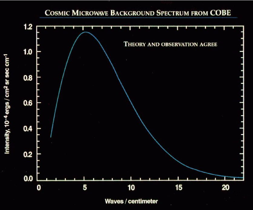
Figure 1: The cosmic background spectrum is that of a near perfect blackbody as predicted by theory. The above graph represents the most recent observations by a number of collaborations. Graph courtesy of COBE Project (cobe, )

The first successful measurement of the CBR was made in 1964 by Penzias and Wilson, two scientists working on a satellite development project for Bell Labs (partridge, ). Their measurements revealed that the CBR was characteristic of a black-body with a corresponding temperature of around $3K$ as illustrated in Figure (1) (partridge, ). The measured wavelengths were on the order of $7.35$ cm, corresponding to the microwave range of the electromagnetic spectrum. The CBR in this range is referred to as the Cosmic Microwave Background (CMB).

Another important observation of Penzias and Wilson is the fact that the CMB is uniform (homogeneous) in all directions (isotropic). Thus, the CMB offers an experimental proof of the isotropy and homogeneity of the universe.

Because of its importance, further measurements of the CBR have been carried out. One such project named COBE, for Cosmic Background Explorer, in $1989$, measured the CBR to have a temperature of $2.73$ K and a distribution that is isotropic to one part in $10^{5}$ (turner, ). COBE also has the distinction of being the first satellite dedicated solely to cosmology. Future measurements will be made by dedicated satellites like COBE, but these satellites will have much higher angular resolution. They are planned to be launched around the beginning of the century.

Balloon born experiments have been able to measure the background spectrum with greater resolution than COBE and the preliminary results seem to favor the type of spectrum predicted by the inflationary scenario, to be discussed later (Melchiorri:1999br, ),(Lange:2000iq, ). Several satellite projects are planned, MAP, for Microwave Anisotropy Probe will be launched at the end of this year by NASA and another named the PLANCK Explorer is planned for launched by the European Space Agency around the year 2006. The accurate measurement of the CBR offers an observational test of cosmological models, as well as, the CP.

In addition to these benefits of CBR observations, the CBR can also be used to setup a Cosmic Rest Frame (CRF). This concept is reminiscent to the ideas of Ernst Mach. One chooses a reference frame to coincide with the Hubble expansion, i.e., with the motion of the average distribution of matter in the universe. It is convenient to define our coordinates in this frame to save confusion in measurements such as the expansion of spacetime and the Hubble Constant; however, these coordinates are in no way ‘absolute’ coordinates. Using the CBR to define the CRF and taking galaxies as the test particles of the model serves to greatly simplify the dynamics in an expanding universe. The CRF is used to ease calculations and make the interpretation of the dynamics of an expanding universe more tractable.

The current and proposed measurements of the CBR offer a convincing test of the homogeneity of space. Measurements of the temperature of the CBR are uniform to one part in $10^{5}$. This suggests the universe is homogeneous and isotropic to a high degree of accuracy. However, since this measurement is taken from our (the Earth’s) vantage point, one can not assume the same conclusion from another vantage point. This can be remedied by considering how the CBR is related to the distribution of matter at the time the photons of the CBR decoupled. This offers a ‘snap shot’ of the inhomogeneities in the density of the universe. If these regions contained more inhomogeneity, galaxies would not be visible today. This idea will be discussed in more detail later; as an alternative one can introduce the Copernican Principle (CP).

The CP states that no observers occupy a special place in the universe. This appears to be a favorable prediction, based on the evidence above, as well as lessons coming from the past. For example, the correct model of the solar system was not realized until humans realized they were not the center of the solar system. This may be a bit humbling to the human ego, but the Copernican Principle, along with homogeneity and isotropy, serve to greatly simplify the number of possible cosmological models for the universe. Later, it will be seen that homogeneity follows naturally from inflation. If the universe went through a brief period of rapid expansion, the fact that galaxies exist at all will be a necessary and sufficient condition for a homogeneous universe.

There is also the proposal for cosmic ‘no-hair’ theorems. These theorems are similar to the ‘no-hair’ proposal of black holes, which predict that any object that contains an event horizon will yield a Schwartzschild spherically symmetric solution at the singularity. The Big-Bang singularity is no exception, and the event horizon is the Hubble distance to be explored in sections to come. For now, experiment suggests that it is safe to assume the Copernican Principle is valid.

Below is a brief descriptive summary of observational methods for testing the CP:

• Particle Backgrounds – These observations represent the strongest argument for isotropy and homogeneity. As the universe evolved it cooled allowing various particle species to become ‘frozen out’, meaning that the particles were freed from interactions. Photons, for example, became frozen out at the time of decoupling and are visible today as the CBR. These backgrounds serve as an important experimental test for predictions by various cosmological models.

• The Observed Hubble Law – This law states that the farther away a galaxy is, the faster it will be observed to recede. This phenomena is observed through a redshift of the light coming from the galaxy and will be described in a later section. The observed redshift, first witnessed by Edwin Hubble was the first indication that the universe obeys the CP.

• Source Number Counts – Of all methods this is the most uncertain at this time. This method requires collecting light from galaxies and inferring whether ‘clustering’ occurs. One debate over the accuracy of such methods is based on the idea that most matter in the universe might be of a non-luminous type, the so-called Dark Matter. Another problem is that current technology does not allow observations at distances far enough to get a good sample of the population. However, this technique shows promise for the future, and the SLOAN Digital Sky Survey is a current project that will map in detail one-quarter of the entire sky, determining the positions and absolute brightness of more than $100$ million celestial objects. It will also measure the distances to more than a million galaxies and quasars.

• Inflation – Although it is premature at this point to discuss observational consequences of inflation, it will be shown that inflation predicts small perturbations in the universe that result in the large-scale structure observed today. It will be shown that if these perturbations were too large then the structure we observe today would not be possible. Thus, if inflation can be proved through observation, it would imply the universe must have been very homogeneous at the time of decoupling.

The established concepts of the CP aid in simplification of cosmological models, but a further simplification can be made by invoking the Perfect Cosmological Principle. This principle differs from the previous one in that it assumes temporal homogeneity and isotropy. This would imply a static universe, for if the universe were expanding or contracting it would not look the same now, as it did in the past. However, one exception that will prove important later is the case of a (anti or quasi) DeSitter Space. By the observations of Edwin Hubble and the theoretical work by Lamaître it was shown that the expansion of the universe is an accurate assumption. CP models further suggest that a static universe would be as stable as a pencil standing on its end. Thus, the Perfect Cosmological Principle does not appear to be an acceptable assumption within the standard model (hawking, ).

The last element to be discussed concerning the CP is the Weyl Postulate. This postulate formally states that, “the world lines of galaxies designated as ‘test particles’ form a 3-bundle of nonintersecting geodesics orthogonal to a series of spacelike hypersurfaces” (narlikar, ). In other words, the geodesics on which galaxies travel do not intersect. This adds another symmetry to the picture of the expanding universe allowing simplification of the spacetime metric and the Einstein equations.

II.2 The Expanding Universe

In the mid-twenties, Edwin Hubble was observing a group of objects known as spiral nebulae. These nebulae contain a very important class of stars known as Cepheid Variables. Because the Cepheids have a characteristic variation in brightness (bergstrom, ), Hubble could recognize these stars at great distances and then compare their observed luminosity to their known luminosity. This allowed him to compute the distance to the stars, since luminosity is inversely proportional to the square of the distance (bergstrom, ). The intrinsic, or absolute, luminosity is calculated from simple models that have been commensurate with observations of near Cepheids.

When Hubble compared the distance of the Cepheids to their velocities (computed by the redshift of their spectrum) he found a simple linear relationship,

$${\vec{V}_{H}}=H\vec{r},$$ (1)

where ${\vec{V}_{H}}$ is the velocity of the galaxy, $H$ is the so-called Hubble Constant, and $\vec{r}$ is the displacement of the galaxy from the Earth. It will be shown later that the Hubble constant is not actually a constant, but can be a function of time depending on the chosen model. The standard notation is to adopt $H_{0}$ as the ‘current’ observed Hubble parameter, whereas $H=H(t)$ is referred to as the Hubble constant. The current accepted value of the Hubble parameter is,

$$H_{0}=100h_{0}\;\mbox{km}\cdot\mbox{s}^{-1}\cdot\mbox{Mpc}^{-1}\;\;\;\;\;\mbox{where}\;\;0.5<h_{0}<0.8.$$ (2)

The unit of length, Mpc, stands for Megaparsec.

Hubble’s interpretation of his data was crucial in helping determine the correct model for the universe. Hubble had found that the galaxies, on average, were receding away from us at a velocity proportional to their distance from us (1). This suggests a homogeneous, isotropic, and expanding universe. By this finding, the choices of cosmological models became greatly restricted.

Perhaps it is worth mentioning that the above analysis by Hubble is not quite as easily done as one might think. One factor that must be considered in the calculation of the Hubble velocity field (1) is the concept of peculiar velocity. This is the name given to the motion of a galaxy, relative to the CRF, due to its rotation and motion as influenced by the gravitational pull of nearby clusters. This speed, $v_{p}\leq\pm 500\;\mbox{km}\cdot\mbox{s}^{-1}$, can be neglected at far distances where the Hubble speed, ${V_{H}}\gg 500\;\mbox{km}\cdot\mbox{s}^{-1}$. Thus, when Hubble conducted his survey most of the nebulae were too near to rule out an effect by the peculiar velocity. As a result, Hubble found $H_{0}\approx 500\;\mbox{km}\cdot\mbox{s}^{-1}\cdot\mbox{Mpc}$, much greater than the value obtained today from surveys of type Ia supernovae.

II.2.1 The Hubble Law and Particle Kinematics

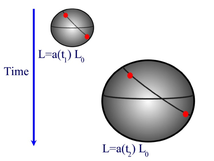
Figure 2: As the universe expands the distance between galaxies (test particles) increases proportional to the scale factor, $L(t)=a(t)L_{0}$.

The Hubble law (1) is a direct result of the CP. Consider the expansion of the universe, which must occur in a homogeneous and isotropic manner according to the CP. The expansion can be visualized with the analogy of a balloon with a grid painted on it. Of course this should not be taken literally, since the spatial extent of the universe is three dimensional. Think of the grid as a network of meter sticks and clocks at rest with respect to the Hubble expansion, which corresponds to the Cosmic Rest Frame (CRF) mentioned earlier. Due to the expansion, two particles initially separated by a distance $l_{0}$, will be separated by a distance $l(t)=a(t)l_{0}$ at some later time $t$, see Figure (2). Because of the CP, the function $a(t)$, known as the scale factor, can only be a function of time. From this relation, the speed of the observers relative to each other is,

$$v(t)=\frac{dl}{dt}=\dot{a}l_{0}=\Big{(}\frac{\dot{a}}{a}\Big{)}l(t)=H(t)l(t),$$

where $\dot{a}$ is the time derivative of the scale factor.

From this derivation of the Hubble law, it becomes manifest that the Hubble Constant can depend on time. In this new way of defining $H(t)=\dot{a}(t)/a(t)$, $H(t)$ measures the rate of change of the scale factor, $a(t)$, and offers a way to link observations (like Hubble’s) with a proposed model using the scale factor. For Hubble’s observations, the distance $l(t)$ was small and $H(t)$ could be estimated by a linear relation yielding equation (1).

To understand how particles ‘come to rest’ in the CRF, consider a particle starting out with a peculiar velocity $v_{p}\ll c$. The particle passes a CRF observer ($O_{1}$) at time $t$ and travels a distance $dl=v_{p}\>dt$. At this time the particle passes another CRF observer ($O_{2}$), who has a velocity $dv=Hdl=Hv_{p}\>dt$ relative to $O_{1}$. $O_{2}$ measures the particle’s peculiar velocity as, $v_{p}(t+dt)=v_{p}(t)-dv$. This shows that the peculiar velocity satisfies the equation of motion,

$$\frac{dv_{p}}{dt}=-\frac{dv}{dt}=-Hv_{p}=-\Big{(}\frac{\dot{a}}{a}\Big{)}v_{p}.$$ (3)

Solving this differential equation yields,

$$v_{p}\propto\frac{1}{a}\;.$$

This indicates that the peculiar velocity decreases as the scale factor increases. Indicating that as the universe expands, particles with peculiar velocities tend to go to zero meaning they ‘settle’ into the CRF.

II.2.2 The Robertson Walker Metric

The only metric compatible with Hubble’s findings and the Cosmological Principle is the Robertson Walker Metric (RWM) with the corresponding line element,

$$ds^{2}=c^{2}dt^{2}-a^{2}(t)\left[\frac{dr^{2}}{1-kr^{2}}+r^{2}d\theta^{2}+r^{2}\sin^{2}{\theta}d\phi^{2}\right].$$ (4)

For a brief explanation consider the following:

• For the metric to be homogeneous, isotropic, and obey the Weyl postulate, the metric must be the same in all directions and locations,

  $$g_{\mu\nu}=g_{\mu\mu}.$$

• For a uniform expansion we must have a scale factor $a(t)$ that is a function of time only.

• Allowance for any type of geometry (curvature) must be made. This is represented by the constant $k$, where $k=0,k=1,$ and $k=-1$ corresponds to flat, spherical, and hyperbolic geometries, respectively.

There are a few subtleties that must be discussed. First, the $r$ that appears in the line element (4) is not the radius of the universe. The $r$ is a dimensionless, comoving coordinate that ranges from zero to one for $k=1$. The measurable, physical distance is given by the RWM above. Choosing a frame common to two distinct points, one obtains,

$$ds^{2}=c^{2}dt^{2}-a^{2}(t)(1-kr^{2})^{-1}dr^{2},$$

for their separation. Where $d\theta$ and $d\phi$ are zero, because one has freedom to arrange the axis and $ds^{2}$ represents their separation in spacetime. Thus, their spatial separation is found by considering spacelike hypersurfaces, that is $dt^{2}=0$. Thus, their separation is

$$d_{p}=a(t)\int_{0}^{r}(1-kr^{2})^{-1/2}\;dr.$$

Evidently for a $k=0$ flat universe, the distance is simply,

$$d_{p}=a(t)r.$$ (5)

Thus, $a(t)$ has units of length and depends on the geometry of the spacetime.

The next issue is that of curvature. The curvature of the universe is determined by the amount of energy and matter that is present. The space is one of constant curvature determined by the value of $k$. Because any arbitrary scaling of the line element (4) will not affect the sign of $k$, we have the following convention:

• k=1 represents positive, spherical geometry

• k=0 represents flat Minkowski space

• k=-1 represents negative, hyperbolic geometry

II.2.3 The Cosmological redshift

One observable prediction of an expanding universe is that of redshifting. When a light wave is traveling from a distant galaxy, to our own, it must travel through the intervening spacetime. This results in a stretching of the wavelength of light, since the spacetime is expanding. This longer wavelength results in the light being shifted to a ‘redder’ part of the spectrum. Of course light with wavelengths differing from visible light will not be visible to the human eye, but they will still be shifted to longer wavelengths.

To quantify this analysis, consider a light ray which must travel along a null geodesic ($ds^{2}=0$) in the comoving frame with constant $\theta$ and $\phi$. Using (4),

$$0=ds^{2}=c^{2}dt^{2}-a^{2}(t)\Big{[}\frac{dr^{2}}{1-kr^{2}}\Big{]},$$

so,

$$c\>dt=\frac{a(t)dr}{\sqrt{1-kr^{2}}}.$$

Integrating yields,

$$\int_{t_{e}}^{t_{0}}\frac{c\>dt}{a(t)}=\int_{0}^{r_{e}}\frac{dr}{\sqrt{1-kr^{2}}}\equiv f(r_{e}),$$ (6)

where $t_{e}$ is the time the light pulse was emitted, $t_{0}$ was the time the light pulse was received, and $r_{e}$ is the distance to the galaxy. Thus, if one knows $a(t)$ and $k$, one can find the relation between the distance and the time. However, consider emitting successive wave crests in such a brief time that $a(t)$ is not given a chance to increase by a significant amount; i.e., the waves are sent out at times $t_{e}$ and $t_{e}+\Delta t_{e}$ and received at times $t_{0}$ and $t_{0}+\Delta t_{0}$, respectively. Then (6) becomes,

$$\int_{t_{e}+\Delta t_{0}}^{t_{0}+\Delta t_{e}}\frac{c\>dt}{a(t)}=\int_{0}^{r_{e}}\frac{dr}{\sqrt{1-kr^{2}}}$$

Subtracting (6) from this equation and using the fact $a(t)$ doesn’t change, one can use the fundamental theorem of calculus to obtain,

$$\frac{c\>\Delta t_{0}}{a(t_{0})}-\frac{c\>\Delta t_{e}}{a(t_{e})}=0,$$

or

$$\frac{c\>\Delta t_{0}}{c\>\Delta t_{e}}=\frac{a(t_{0})}{a(t_{e})}.$$

$c\>\Delta t$ is just the wavelength, $\lambda$. Thus, it follows that the red shift, $z$, can be defined by

$$z=\frac{a(t_{0})}{a(t_{e})}-1=\frac{\lambda_{0}}{\lambda_{e}}-1=\frac{\Delta\lambda}{\lambda_{e}}.$$ (7)

Here $a(t_{0})$ is the scale factor of the universe as measured by a comoving observer when the light is received, $a(t_{e})$ is the scale factor when the light was emitted in the comoving frame, $\lambda_{0}$ is the wavelength observed and $\lambda_{e}$ is the wavelength when emitted. It is clear that $z$ will be positive, since $a(t_{0})>a(t_{e})$, that is the universe is getting larger.

In addition to this cosmological redshift, which is due to the expanding universe, there can also be gravitational redshifts and Doppler redshifts. At great distances the former two can be neglected, but in local cases all three must be considered.

It must also be stressed that the Special Relativity (SR) formula for redshift can not be used. This is because SR only holds for ‘local’ physics. Attempting to use this across large distances can result in a contradiction. For example, the expansion rate of the universe can actually exceed the speed of light at great distances. This is not a violation of SR, because a ‘chain’ of comoving particles (galaxies) can be put together, spaced so the laws of SR are not violated. By summing together the measurements of each set of galaxies, one finds the expansion rate to exceed that of light, although locally SR holds locally (bergstrom, ). Another explanation is that in a universe described by SR, no matter or energy exists and the metric never changes. On the contrary, in an expanding spacetime none of these requirements are true. Although, SR continues to hold locally, since a ‘small enough’ region can always be chosen where the metric is approximately flat.

II.3 The Friedmann Models

To describe the expansion of the universe one must use the RWM along with the Einstein equations,

$$R_{\mu\nu}-\frac{1}{2}g_{\mu\nu}R+\frac{\Lambda g_{\mu\nu}}{c^{2}}=-\frac{8\pi G}{c^{4}}T_{\mu\nu},$$ (8)

to determine the equations of motion. For reference, a summary of the metric coefficients, the Christoffel Symbols, and the Ricci Tensor components are presented in (collins, , Chapter 15). Note that in this book the scale factor $a(t)$ is written $R(t)$.

Before proceeding any further, an appropriate stress-energy tensor must be provided. This is the difficult part of the process. The composition of the known universe is a very controversial topic. The standard procedure is to consider simplified distributions of mass and energy to get an approximate model for how the universe evolves.

At this point, units are chosen such that the speed of light, $c$ is set equal to unity. This gives the simplification that the energy density, $\epsilon$ is equal to the mass density, $\rho$ using, $\epsilon=\rho c^{2}=\rho.$ This also allows mass and energy to be considered together, which is in the spirit of the stress-energy tensor. The mass/energy density will be referred to as the energy density for the remainder of this paper. The stress-energy tensor may be given as:

$$T_{\mu\nu}=(p+\rho)u_{\mu}u_{\nu}-pg_{\mu\nu},$$ (9)

where $p$ is the pressure, $\rho$ is the density, and $u_{\mu}$ is the four-velocity.

At the earliest epoch of the universe, the contribution of photons to the energy density would have been appreciable. However, as the universe cooled below a critical temperature, allowing the photons to decouple from baryonic matter, the photon contribution became negligible. Thus, it is easier to consider different energy distributions for different epochs in the universe. The massive contribution to the energy density is usually referred to as the Baryonic contribution, since baryons (protons, neutrons, etc.) are significantly more massive than leptons (electrons, positrons, etc.) and leptons can therefore be disregarded as a major contributing factor to the total energy density. There is also the contribution of vacuum energy, which enters the Einstein equations through the cosmological constant, $\Lambda$.

For each type of contribution, there is a corresponding density, $\rho$. The total density can be expressed as the sum of the different contributions as

$$\rho=\rho_{M}+\rho_{R}+\rho_{\Lambda}.$$ (10)

Furthermore, assuming that one is dealing with a homogeneous and isotropic fluid, the density can be related to the pressure by a simple equation of state (see Table 1),

$$p=\alpha\rho.$$ (11)

Another useful relation involves the Conservation of Energy (1st Law of Thermodynamics). Assuming the ideal fluid expands adiabatically, one finds (finkelstein, ),

$$dE=-p\>dV,$$

which may be rewritten as,

$$d(\rho a^{3})=-pd(a^{3}).$$ (12)

Relating (11) and (12) gives,

$$d(\rho a^{3})=-\alpha\rho d(a^{3}).$$

Using the product rule,

$$\rho d(a^{3})+a^{3}d\rho=-\alpha\rho d(a^{3}).$$

Which can be integrated,

$$\int\rho^{-1}d\rho=-(1+\alpha)\int a^{-3}d(a^{3}).$$

$$\rho\propto a^{-3(1+\alpha)}.$$ (13)

In the Radiation epoch, where the energy density due to photons was appreciable (from about $t$=0 to approximately 300,000 years after the Big-Bang (dekel, )), the density due to massive particles can be neglected. The pressure is found to be equal to a third of the density, and we have a value of one-third for $\alpha$, so $\rho_{R}\sim a^{-4}$ (bergstrom, ).

Following this epoch, the Matter Dominated epoch can be modeled after a ‘dust’ that uniformly fills space. Because the temperature of the universe had fallen to around 3000 K, most of the particles had non-relativistic velocities ($v\ll c$). This corresponds to a negligible pressure and $\alpha$ is therefore zero, $\rho_{\Lambda}\sim\mbox{constant}$ (bergstrom, ).

The last case to consider is that of the vacuum energy. If the cosmological constant is indeed nonzero, this form of energy density will dominate. For this relation, the pressure is commensurate with that of a negative density. This would imply a value of -1 for $\alpha$, so $\rho_{M}\sim a^{-3}$ (bergstrom, ). These results are summarized in Table 1.

Given an expression for the energy-momentum tensor, one can now proceed to find the equations of motion. The metric coefficients follow from the Robertson Walker line element, which is given by equation (4). Using these coefficients one can obtain the expression for the left side of the Einstein equations (8). Thus, from the Einstein equations one derives the Friedmann equations in their most general form:

$$\frac{\ddot{a}}{a}=-\frac{4\pi G}{3}\Big{(}\rho+3p\Big{)}+\frac{\Lambda}{3},$$ (14)

$$\Big{(}\frac{\dot{a}}{a}\Big{)}^{2}=\frac{8\pi G\rho}{3}-\frac{k}{a^{2}}+\frac{\Lambda}{3}.$$ (15)

Apparently, if the universe is in a vacuum dominated state $p=-\rho$, (14) indicates the universe will be accelerating. This important conclusion will be the most general requirement for an inflationary model.

Now is the time to introduce a bit of machinery to make our calculations more tractable. Recall that the Hubble constant, $H(t)$, is defined as

$$H(t)=\frac{{\dot{a}(t)}}{a(t)}.$$ (16)

Next, one defines the Deceleration parameter (named for historical reasons) as,

$$q(t)=-\frac{\ddot{a}(t)}{a(t)H^{2}(t)}.$$ (17)

To realize how this term arises, consider the Taylor expansion of the scale factor, about the present time, $t_{0}$,

$$a(t)=a_{0}+\dot{a}_{0}(t-t_{0})+\frac{1}{2}\ddot{a}_{0}(t-t_{0})^{2}+\ldots,$$

where the sub-zeros indicate the terms are evaluated at the present. Using equations (16) and (17), this becomes

$$a(t)=a_{0}\big{[}1+H_{0}(t-t_{0})-\frac{1}{2}q_{0}H_{0}^{2}(t-t_{0})^{2}+\ldots\big{]}.$$ (18)

Remembering that the crux for obtaining Hubble’s Law (1) was measuring the luminosity distance, it is of interest to consider this calculation quantitatively. The flux $F$ (energy per time per area received by the detector) is defined in terms of the known luminosity $L$ (energy per time emitted in the star’s rest frame) and the luminosity distance $d_{L}$.

$$F=\frac{L}{4\pi d^{2}_{L}}.$$ (19)

The luminosity distance must take into account the expanding universe and can be written in terms of the redshift, $z$ as (turner, ),

$$d^{2}_{L}=a^{2}_{0}r^{2}(1+z)^{2},$$ (20)

where $a_{0}$ is the present scale factor and $r$ is the comoving coordinate that parameterizes the space. Hubble used the measured flux and the known luminosity to find the distance to the objects he measured. The distance can then be compared with the known redshift of the object using (20) and the velocity can be approximated. However, $r$ in (20) is not a observable and it is of interest to examine the great amount of estimation that must be used to derive the desired result analytically.

Dividing (18) by $a_{0}$ and making use of (7) yields,

$$\frac{a_{0}}{a}=z=H_{0}(t_{0}-t)+\Big{(}1+\frac{q_{0}}{2}\Big{)}H^{2}_{0}(t_{0}-t)^{2}+\ldots,$$ (21)

which can be solved for $(t_{0}-t)$,

$$(t_{0}-t)=H_{0}^{-1}\Bigg{[}z-\Big{(}1+\frac{q_{0}}{2}\Big{)}z^{2}+\ldots\Bigg{]}.$$ (22)

One can also expand (6) in a power series,

$$f(r)=sinn^{-1}(r),$$ (23)

where $r_{e}$ has been replaced by $r$ (for simplicity) and $sinn^{-1}(r)$ is defined as $sin^{1}(r)$ for $k=1$, $sinh^{-1}(r)$ for $k=-1$ and $r$ for $k=0$. So to lowest order, (6) can be estimated as $r$, and the l.h.s. of (6) can be estimated as,

$$\int^{t_{0}}_{t_{e}}\frac{c\;dt}{a(t)}\approx\frac{c(t-t_{0})}{a_{0}}.$$ (24)

Using the approximation from (23) and the above result we have,

$$\frac{c(t-t_{0})}{a_{0}}\approx r.$$

Substitution of $t-t_{0}$ from (22) and keeping only lowest order terms yields,

$$a_{0}r\approx c(t-t_{0})\approx\frac{cz}{H_{0}}.$$

At small redshift, $z\ll 1$ one finds $z\approx v/c$. Thus, making this final approximation one obtains,

$$cz\approx v\approx a_{0}H_{0}r\approx H_{0}d_{p},$$ (25)

$$v\approx H_{0}d_{p},$$ (26)

where $d_{p}$ is the physical distance. Thus, we have obtained Hubble’s law (1) as an approximation. This derivation reflects the reason that the law only holds locally. The number of approximations that were needed to proceed was appreciable. Furthermore, one finds that this law deviates significantly at large $z$ as one would expect.

For a matter dominated model, one finds the exact Hubble relation to be given by (turner, ),

$$H_{0}d_{l}=q_{0}^{-2}\Bigg{[}zq_{0}+(q_{0}-1)\Big{(}\sqrt{2q_{0}z+1}-1\Big{)}\Bigg{]},$$ (27)

which depends on the deceleration parameter, $q_{0}$, which in turn relies on the curvature and the total mass density of the universe.

II.4 Matter Dominated Models

The present epoch is best described by a matter dominated universe, so it is perhaps best to explore this model first. Again, matter domination corresponds to a non-relativistic, homogeneous, isotropic ‘dust’ filled universe with zero pressure. By setting $p=0$ in (15) and incorporating the $\Lambda$ term into a total density, $\rho_{T}=\rho+\frac{\Lambda}{8\pi G}$, the Friedmann equations for a matter dominated universe emerge,

$$\Big{(}\frac{\dot{a}}{a}\Big{)}^{2}+\frac{k}{a^{2}}=\frac{8\pi G\rho_{T}}{3}.$$ (28)

$$2\frac{\ddot{a}}{a}+\Big{(}\frac{\dot{a}}{a}\Big{)}^{2}+\frac{k}{a^{2}}=0.$$ (29)

Again, the value of $k$ describes the geometry of the space. Equation (29) is actually obtained by combining (14) and (15) and is often called the acceleration equation.

The idea of the total density, $\rho_{T}$, might be a bit confusing since it has been stated that the model is matter dominated. Although this is true, there can still be a small contribution in the form of radiation and other forms of energy, such as dark matter. The point is that any of these should be much less than $\rho_{M}$ for the model to be accurate. It will also be seen that $\rho_{M}$ can also be broken into different contributions as tacitly stated in the previous remark about dark matter. For the remainder of this section we take $\rho$ to mean $\rho_{T}$ to keep the notation as simple as possible.

II.4.1 The Einstein-DeSitter Model

The Einstein-DeSitter model is a matter dominated Friedmann model with zero curvature ($k=0$). This model corresponds to a Minkowski universe (zero curvature), in which the universe will continue to expand forever with just the right amount of energy to escape to infinity. It is analogous to launching a rocket. If the rocket is given insufficient energy, it will be pulled back by the Earth. However, if its energy exceeds a certain critical velocity (escape velocity), it will continue into space with ever increasing speed. If it has exactly the escape velocity, it will proceed to escape the Earth with a velocity going to zero as the rocket approaches spatial infinity. The Einstein-DeSitter model corresponds to the universe having exactly the right escape velocity provided by the Big-Bang to escape the pull of gravity due to the matter in the universe.

By substituting $k=0$ into (29) and (28), the Friedmann equations become

$$0=2\frac{\ddot{a}}{a}+\Bigg{(}\frac{\dot{a}}{a}\Bigg{)}^{2}=-2q(t)H^{2}(t)+H^{2}(t),$$ (30)

$$\Bigg{(}\frac{\dot{a}}{a}\Bigg{)}^{2}=H(t)^{2}=\frac{8\pi G\rho}{3}.$$ (31)

By solving (31) for $\rho$, a critical density can be found for a flat universe. The critical density is the amount of matter required for the universe to be exactly flat ($k=0$) and is a function of time. The critical density at the present is defined as,

$$\rho_{c}=\frac{3H^{2}_{0}}{8\pi G}.$$ (32)

If the density of the universe exceeds the critical density, the universe is open. Conversely, if the density is below $\rho_{c}$ the universe is open. For the observed Hubble parameter as defined in (2), the critical density today corresponds to a value,

$$\rho_{c}\approx 2\>h_{0}^{2}\times 10^{-23}\frac{\mbox{g}}{\mbox{m}^{3}}.$$ (33)

This is equivalent to roughly 10 hydrogen atoms per cubic meter. Although, this is incredibly small compared to Earthly standards, it must be remembered that most of space is empty and the concern is the total energy density.

Notice that the critical density depends on the Hubble constant. This means that the density required for a flat universe will change with time, in general, as the universe expands. For the universe to be ‘fine-tuned’ to this precision is highly improbable; yet, most observations suggest this type of geometry. This paradoxical issue is referred to as the Flatness problem and will lead to one of the claimed triumphs of Inflation theory. Because it is believed that the universe is so close to being flat, it is useful to define the density parameter, $\Omega$. $\Omega_{0}$ is the ratio of the density observed today, $\rho_{0}$, to the critical density, $\rho_{c}$. In general, $\Omega$ is the ratio of the density to the critical value.

The quantity $\Omega$ together with Equation (30), which implies $q_{0}=\frac{1}{2}$, can be used to discriminate between the possible geometries for the matter dominated universe (see Table 2).

From the previous result for a matter dominated energy density, we found $\rho\sim a^{-3}$. From this relation, conservation of energy follows,

$$\frac{d}{dt}(\rho a^{3})=0\Rightarrow\rho a^{3}=\mbox{constant}.$$

This can be used to obtain a useful relation for $\rho$,

$$\rho=\rho_{0}\frac{a^{3}_{0}}{a^{3}}.$$

Returning to the Friedmann equation (31) and substituting the above expression for $\rho$ one finds,

$$\Bigg{(}\frac{\dot{a}}{a}\Bigg{)}^{2}=\frac{8\pi G\rho}{3}=\frac{8\pi G\rho_{0}}{3}\frac{a^{3}_{0}}{a^{3}}.$$

Combining terms in $a$,

$$a\dot{a}^{2}=\frac{8\pi G\rho_{0}a_{0}^{3}}{3},$$

now integrating,

$$\int_{0}^{a}\sqrt{a}da=\int_{0}^{t}\sqrt{\frac{8\pi G\rho_{0}a_{0}^{3}}{3}}dt,$$

$$a(t)=a_{0}\Bigg{(}\frac{8\pi G\rho_{0}}{3}\Bigg{)}^{\frac{1}{3}}t^{\frac{2}{3}},$$

$$a\propto t^{2/3}.$$ (34)

So for the Einstein-DeSitter Model, the scale factor evolves as $t^{2/3}$.

II.4.2 The Closed Model

The Closed Model is characterized by a positive curvature, $k=1$. Thus, the spatial structure is that of the 3-sphere, similar to the surface of a sphere, but in 3 dimensions instead of 2. This model corresponds to a universe that begins at a ‘Big-Bang’ and continues to expand until gravity finally halts the expansion. The universe will then collapse into a ‘Big-Crunch’, which will resemble the reverse process of the ‘Big-Bang’. The ability of the matter (or energy) in the universe to halt the expansion obviously depends on the density. If the matter-energy density is too low, the universe will have enough momentum from the ‘bang’ to escape the pull of gravity. In the Closed Model the density of the universe is great enough to halt the expansion and start a contraction. This corresponds to a value of $\Omega>1$, which is evident from the use of the Friedmann equations with $k=1$. Plugging this $k$ value into the Friedmann equations (29),(28) and using $\ddot{a}=-qH^{2}a$ one gets,

$$2\frac{\ddot{a}}{a}+\frac{{\dot{a}}^{2}}{a^{2}}+\frac{1}{a^{2}}=2\Big{(}-qH^{2}\Big{)}+H^{2}+\frac{1}{a^{2}}=0.$$

This can be expressed as

$$\frac{1}{a^{2}}=H^{2}\Big{[}2q-1\Big{]}.$$ (35)

Equation (28) takes the form,

$$\frac{{\dot{a}}^{2}}{a^{2}}+\frac{1}{a^{2}}=\frac{8\pi G\rho}{3}.$$ (36)

Combining (35) and (36) gives,

$$H^{2}+\Bigg{[}H^{2}\Big{(}2q-1\Big{)}\Bigg{]}=\frac{8\pi G\rho}{3},$$

or

$$2qH^{2}=\frac{8\pi G\rho}{3}.$$

Thus,

$$\rho=\frac{3H^{2}q}{4\pi G}.$$ (37)

Comparing (37) with the critical density (32) and the value of $q>1/2$ in Table 2, it is evident that $\rho>\rho_{c}$ for the universe to be closed. In terms of $\Omega$, this gives

$$\Omega=\frac{\rho}{\rho_{c}}>1.$$ (38)

The advantage of equation (37) above, is that the density is expressed all in quantities that can be measured. In that, if 2 of the 3 quantities are known the third may be found.

II.4.3 The Open Model

The so-called Open Model is the case where $k=-1$ and the geometry is said to be hyperbolic. Taking $k=-1$ in the Friedmann equations (29),(28),

$$2\frac{\ddot{a}}{a}+\frac{{\dot{a}}^{2}}{a^{2}}-\frac{1}{a^{2}}=0.$$ (39)

$$\frac{\dot{a}^{2}}{a^{2}}-\frac{1}{a^{2}}=\frac{8\pi G\rho}{3}$$ (40)

Solving these equations (39),(40) yields the same value of the density (37) as the closed model, but in this case $q<1/2$ and $\Omega<1$, as previously discussed.

II.5 Summary

• All cosmological models are characterized by ‘test particles’, which are galaxies that are distributed in a homogeneous and isotropic manner in accordance with the CP.

• Open Models are characterized by $\Omega<1$, negative curvature ($k=-1$), hyperbolic geometry, a deceleration parameter $q<1/2$, and infinite spatial extent (ignoring topology).

• Closed Models are characterized by $\Omega>1$, positive curvature ($k=1$), spherical geometry, a deceleration parameter $q>1/2$ and finite spatial extent.

• Flat Models are characterized by $\Omega=1$, flat geometry with no curvature ($k=0$), infinite spatial extent, a deceleration parameter $q=1/2$ and with an age corresponding to Age=$H_{0}^{-1}$, since the Hubble Constant is in-fact constant.

III A Brief History of the Universe

One of the successes of the hot Big Bang model is its prediction of the light elements. These predictions are verified by observations of the structure and composition of the oldest stars, quasars, and other quasi-stellar remnants (e.g., QSOs) (9907128, ; 9904407, ; 9712031, ; 9904223, ). The process by which the elements form is referred to as nucleosynthesis.

The Hot Big-Bang model predicts a universe that will go through several stages of thermal evolution. As the universe expands adiabatically, the temperature cools, scaling as

$$T\propto a^{-3(\gamma-1)}.$$

Here $\gamma$ is the ratio of specific heats and is equal to $4/3$ for a radiation dominated universe (peacock, ). This relation is manifest, since the temperature is equivalent to the energy density divided by the volume (in natural units $\hbar=c=k=1$). Moreover, the radiation energy density is redshifted by an additional factor of $1/a(t)$ since the Hubble expansion stretches the wavelength, which is inversely proportional to the energy:

$$\rho_{R}\propto a^{-4},$$

and

$$\rho_{R}=a^{-3}E.$$

Setting the Boltzman constant to unity,

$$E=T\propto a^{-1}.$$ (41)

This can also be understood using the DeBroglie wavelength of the photon (for radiation) (peebles, ). The wavelength is inversely proportional to the energy in natural units. This raises the issue of a possible factor of redshifting for the DeBroglie wavelength of a massive particle. For a particle the simple relation $E=pc$ does not hold; thus, the velocity of the particle can decrease to preserve its wavelength. This redshifting is analogous to that of equation (3) in the first section and gives an alternative explanation of particles in motion settling into the cosmic rest frame. This also explains why one might expect to find primarily non-relativistic (cold) matter, which just means particles traveling at speeds much less than $c$.

From relation (41) for the temperature, one has a quantitative way to find critical temperature scales in the evolution of the universe. For a given value of the curvature the relation between the scale factor and time can yield an expression between temperature and time. For example, in a matter dominated, flat universe,

$$T\propto t^{-2/3},$$

which was derived earlier.

In thermal physics one is usually interested in thermal equilibrium. This consideration is accounted for by the condition,

$$\frac{\Gamma}{H}\gg 1.$$

This relations shows that the reaction rate, $\Gamma$, must be much greater than the rate at which the universe expands for thermal equilibrium to be reached. $\Gamma$ is related to the cross-section of the given particle interaction by

$$\Gamma=n\sigma|v|,$$

where $\sigma$ is the cross-section, $|v|$ is the relative speed, and $n$ is the number density of the species.

From equation (41), one can see that the universe began as a point of infinite temperature and zero size. This is a singular point for the history of the universe and the standard Big Bang model (General Relativity) breaks down at this singularity. However, after the Planck time $(10^{-43})$s one can follow the evolution using the concepts of thermal physics and particle theory.

In the earliest times following the Planck epoch, all matter existed as free quarks and leptons. The existence of free quarks (known as asymptotic freedom) is made possible by the high energy (temperature) during the early moments of the Big Bang. The universe cools, as indicated by (41), and the quarks begin to combine under the action of the strong force to form nucleons. This phase of formation is referred to as Baryogenesis, because the baryons (e.g., protons and neutrons) are created for the first time. The expansion continues to allow leptons, such as electrons, to interact with nucleons to form atoms. At this point, referred to as recombination, the photons in the universe are free to travel with virtually no interactions. For example, hydrogen is the most abundant element to form in nucleosynthesis and at the time of decoupling the temperature of the photons has dropped to around $3000\;K$. This corresponds to less than $13.6\;\mbox{eV}$, the energy needed to ionize the atoms. Therefore, there are no longer free electrons to interact with the photons and in fact the energy of a photon (around $.26\;\mbox{eV}$, at this temperature) is so low that it can not interact with the atoms. In this way the photons have effectively decoupled from matter and travel through the universe as the cosmic background discussed in Part II. A brief summary of the most significant events are encapsulated below,

• $10^{-4}$ seconds: Baryogenesis occurs, quarks condense under strong interaction to form nucleons (e.g., Protons and Neutrons)

• 1 second: Nucleosynthesis occurs, universe cools enough (photon energies $\sim\;1\;\mbox{MeV}$) for light nuclei to form (e.g., deuterons, alpha particles).

• $10^{4}$ years: Radiation density becomes equal to matter density, since the radiation density has extra factor of $a^{-1}$ due to red-shifting. Matter density is the dominate energy density after this epoch.

• $10^{5}$ years: Recombination occurs and electrons are combined with nucleons to form atoms. This time also coincides with the decoupling of photons from matter, giving rise to a surface of last scattering of the cosmic background radiation.

• $10^{10}$ years: The present.

IV Problems with the Standard Cosmology

The hot Big Bang model has been very successful in predicting much of the phenomena observed in the universe today. The model successfully accounts for nucleosynthesis and the relative abundance of the light elements, (e.g., Hydrogen $\sim$ 75%, Helium $\sim 25\%$, Lithium (trace), Berylium (trace)). The prediction of the Cosmic Background Radiation and the fact that the universe is expanding (i.e., The Hubble Law), both represent successful predictions of the Big Bang theory. However, this model suggests questions which it can not answer, which brings about its own demise. These anomalies are discussed in the following sections.

IV.1 The Horizon Problem

Why is the universe so homogeneous and isotropic on large scales? Radiation on opposite sides of the observable universe today appear uniform in temperature. Yet, there was not enough time in the past for the photons to communicate their temperature to the opposing sides of the visible universe (i.e., establish thermal equilibrium). Consider the comoving radius of the causally connected parts of the universe at the time of recombination compared to the comoving radius at the present, found from Equation (6) (remember $c=\hbar=1$).

$$\int_{0}^{t_{rec}}\frac{dt}{a(t)}\;\ll\int_{t_{rec}}^{t_{0}}\frac{dt}{a(t)}.$$ (42)

This means a much larger portion of the universe is visible today, than was visible at recombination when the CBR was ‘released’. So the paradox is how the CBR became homogeneous to 1 part in $10^{5}$ as we discussed in Part II. There was no time for thermal equilibrium to be reached. In fact, any region separated by more than 2 degrees in the sky today would have been causally disconnected at the time of decoupling (liddleeprint, ).

This argument can be made a bit more quantitative by consideration of the entropy, $S$, which indicates the number of states within the model. This can be used as a measure of the size of the particle horizon (turner, ).

$$S^{RD}_{Horizon}=s\frac{4}{3}\pi t^{3}\approx 0.05\>g_{*}^{-1/2}(m_{pl}/T)^{3},$$ (43)

$$S^{MD}_{Horizon}=s\frac{4}{3}\pi t^{3}\approx 3\times 10^{87}(\Omega_{0}h^{2})^{-3/2}(1+z)^{-3/2},$$ (44)

where $m_{pl}$ is the Planck mass, $s$ is the entropy density, $g_{*}$ is the particle degeneracy, and $z$ is the redshift. These equations for the entropy of the horizon in a radiation dominated (43) and matter dominated universe (44), are presented only to motivate the following estimates. For an explanation please consult (turner, ).

At the time of recombination ($z\approx 1100$), when the universe was matter dominated, equation (44) gives a value of about $10^{83}$ states. Compared with a value today of $10^{88}$ states, this is different by a factor of $10^{5}$. Thus, there are approximately $10^{5}$ causally disconnected regions to be accounted for in the observable universe today. The hot Big Bang offers no resolution for this paradox, especially since it is assumed to be an adiabatic (constant entropy) expansion.

IV.2 The Problem of Large-Scale Structure

In contrast to the horizon problem, the fact that the Big Bang predicts no inhomogeneity is a problem as well. How are galactic structures to form in a perfectly homogeneous universe? The fact that galaxies have been shown to cluster locally with great voids on the order of 100 Mpc, is proof of the inhomogeneity of the universe. Moreover, the $10^{-5}$ anisotropies (temperature differences) on angular scales of 10 degrees as measured by the COBE satellite, form a blueprint of the seeds of formation at the time of decoupling. However, there is no mechanism within the Big Bang theory to account for these ‘seeds’, or perturbations, that result in the large-scale structure. Not only does the Big Bang predict homogeneous structure, but it also had to ‘explode’ in just the right way to avoid collapse. This is often called the fine-tuning problem. Cosmologists would like to have a theory that does not require specific parameters to be put in the theory ad hoc. The density, the expansion rate, and the like, prove to be other unfavorable aspects of the hot Big Bang.

IV.3 The Flatness Problem

The flatness problem is another example of a fine-tuning problem. The contribution to the critical density by the baryon density, based on calculations from nucleosynthesis and the observed abundance of light elements, are in good agreement with observations and give $\Omega_{B}<0.1$. The radiation density is negligible and it is believed that non-baryonic dark matter, or quintessence/dark energy (non zero cosmological constant), will contribute the remainder of the critical density, yielding $\Omega=1$. Although, an $\Omega$ anywhere within the range of 1 causes a problem.

The Friedmann equation (28) can be used to take into account how $\Omega$ changes with time. Noting that $H=\dot{a}/a$ and $\Omega=\rho/\rho_{c}$, one can divide (28) by $H^{2}$ to obtain,

$$\mid\Omega(t)-1\mid=\frac{\mid k\mid}{a^{2}H(t)^{2}}.$$

Using the relationships between the scale factor and time,

$$\mbox{Matter Domination:}\;\;\;\;a_{M}\sim t^{2/3},$$

$$\mbox{Radiation Domination:}\;\;\;\;a_{R}\sim t^{1/2},$$

and using the definition of $H$ yields,

$$\mbox{Matter Domination:}\;\;\;\;\mid\Omega(t)-1\mid\sim t^{2/3},$$

$$\mbox{Radiation Domination:}\;\;\;\;\mid\Omega(t)-1\mid\sim t,$$

From these relations one can see that $\Omega$ must be very fine-tuned at early times. For example, requiring $\Omega$ to be one today, corresponds to a value of $\mid\Omega(1)-1\mid\sim 10^{-16}$ at the time of decoupling and a value of $\mid\Omega(10^{-43})-1\mid\sim 10^{-60}$ at the Planck epoch. This value seems unnecessarily contrived and indicates that we live at a very special time in the universe. That is to say, when the universe happens to be flat. An alternative is that the universe has been, is, and always will be flat. However, this is a very special case and it would be nice to have a mechanism that explains why the universe is flat. The Big Bang offers no such explanation.

IV.4 The Monopole Problem

At early times in the expansion ($z>1000$), the physics of the universe is described by particle theory. Many of these theories predict the creation of topological defects. These defects arise when phase transitions occur in particle models. Since the temperature of the universe cools as the expansion proceeds, these phase transitions are natural consequences of symmetry breakings that occur in particle models. Several types of defects are described briefly below (peacock, , Chapter 10),

• Domain Walls – Space divides into connected regions; one region with one phase and the other region exhibiting the other phase. The regions are separated by walls of discontinuity described by a certain energy per unit area.

• Strings – These are linear defects, characterized by some mass per unit length. They can be visualized at the present time as large strings stretched in space that possibly cause galaxies to form into groups. They serve as an alternative to inflation, for explaining the large-scale structure of the universe. However, at the moment they are not favored due to lack of observations of the gravitational-lensing effect they should exhibit.

• Monopoles – These are point defects, where the field points radially away from the defect, which has a characteristic mass. These defects have a magnetic field configuration at infinity that makes them analogous to that of the magnetic monopole, hypothesized by Maxwell and others.

• Textures These objects are hard to visualize and are not expected to form in most theories. One can consider them as a kind of combination of all the other defects.

Out of all these defects, monopoles are the most prevalent in particle theories. It becomes a problem in the hot Big Bang model, when one calculates the number of monopoles produced in events, such as the electroweak symmetry breaking. One finds they would be the dominate matter in the universe. This is contrary to the fact that no monopole has ever been observed, directly or indirectly, by humans. These monopoles would effect the curvature of the universe and in turn the Hubble parameter, galaxy formation, etc. Therefore, unwanted relics, such as monopoles, remain an anomalous component of the hot Big Bang theory.

V The Inflationary Paradigm

In past years, inflation has become more of a scenario than model. A plethora of models have been suggested, all of which share the common feature that the universe goes through a brief period of rapid expansion. This rapid expansion is manifested in the evolution of the scale factor, $a(t)$. In the case of inflation, $a(t)\sim t^{n}$, where $n>1$ and the universe expands faster than light. This does not violate relativity, since the spacetime is the thing expanding (i.e., no information is being transferred). Since $n$ can take on any value greater than one, this is already an example of the flexibility of the theory.

In Section II it was shown by Equation (14) that if an equation of state $p=-\rho$ is achieved and one has a positive cosmological constant, then the universe will accelerate. Incorporating the cosmological constant, $\Lambda$, into an energy density, $\rho_{\Lambda}$, and assuming it is the dominate one can use (15) and (16) to obtain,

$$H^{2}=\Big{(}\frac{\dot{a}}{a}\Big{)}^{2}=\frac{8\pi G\rho_{\Lambda}}{3}-\frac{k}{a^{2}},$$ (45)

One can choose to ignore the curvature term, since one anticipates a large increase in the scale factor. That is, the presence of the scale factor in the denominator of the $-{k}/{a^{2}}$ term in the equation above will leave this term negligible. This is often referred to as the redshifting of the curvature, since the effect of the curvature can be ignored if the scale factor becomes large enough during a period of constant energy density $\rho_{\Lambda}$. This is actually a glimpse of how the flatness problem will be resolved. So, ignoring the curvature term, we have

$$\Big{(}\frac{\dot{a}}{a}\Big{)}^{2}=\frac{8\pi G\rho_{\Lambda}}{3}.$$ (46)

This is a differential equation with the solution,

$$a(t)\sim e^{Ht},$$ (47)

where $H=\Big{(}\frac{8}{3}\pi G\rho_{\Lambda}\Big{)}^{1/2}$ and since $\rho_{\Lambda}$ is a constant, so is $H$. This model is referred to as the DeSitter model. By introducing a negative pressure, the flatness problem is solved. The crux of this argument is that $\rho_{\Lambda}$ is a constant. This comes from the fact that $\rho_{\Lambda}$ is an intrinsic property of the spacetime manifold. As the manifold is stretched, this vacuum energy does not change. Another way this can be explained is by that the Einstein equations are arbitrary up to a constant term $\Lambda$. The disadvantage of this explanation is that it does not manifest the connection between cosmology and particle theory (more on this later).

Since $\rho_{\Lambda}$ is taken to be the dominate form of energy, the other contributions to the density in the Friedmann equation (28) are also redshifted away, since $\rho_{M}\sim a^{-3}$, $\rho_{R}\sim a^{-4}$. This leads to the conclusion that no matter what the initial distribution of $\rho_{T}=\rho_{{M}}+\rho_{R}+\rho_{\Lambda}$, the vacuum energy will eventually dominate. Thus, the assumption of $\rho_{\Lambda}$ domination can actually be relaxed.

So given a constant vacuum term, the DeSitter scenario ‘drives’ the universe to a flat geometry, thus approaching $\rho=\rho_{c}$, where $\rho_{c}$ is the critical density, (i.e., $\rho_{c}={3H^{2}}/{8\pi G}$). This evolution, if allowed to continue, will produce an empty universe with practically no radiation or matter. The fact that we live in a universe that is full of matter and radiation is why the original proposal, by DeSitter, was rejected and forgotten.

The revision of this idea was suggested by Guth in the early 1980’s (guth, ),(guth2, ). The crux to the modern inflationary scenario, in contrast to the DeSitter model, is to limit the amount of time that this rapid expansion (inflation) occurs. Guth explained the physical mechanism for such an inflationary period as corresponding to a phase transition in the early universe. By limiting the time of the quasi-exponential expansion, Guth was able to produce a universe more like our own. Unlike DeSitter’s model, which was based on a pure solution to Einstein’s equations, Guth’s idea was based on ideas from particle physics. Guth was studying a class of grand unified theories (GUTs) and the predictions they make about particle production in the universe. This suggested how cosmology could be united with particle physics in a phenomenological manner, which has become one of the most appreciated beauties in modern physics today.

V.1 Particle Physics and Cosmology

To better understand the motivation behind inflation, it is important to outline a few aspects of particle physics. Often inflation is introduced in an abstract and unaesthetic manner. One speaks of an inflaton field, an arbitrary scalar field, for which there is no physical motivation. This is often the case because this type of introduction requires limited knowledge of the relevant topics. This includes, but is not limited to, the relativistic Schrödinger (Klein-Gordon) equation, the Dirac equation, scalar fields, symmetries, and group theory.

Since this paper is intended for undergraduates, a brief summary is presented on how one can pursue this knowledge in a qualitative and brief manner. A brief overview of the concepts in particle theory will be provided as needed. Thus, the reader is presented with a dilemma. One may choose to pause at this point and do a brief survey of the suggested texts or one may continue and plan to fill in the details at a later time. Both options have their advantages and disadvantages. I chose the former.

From the author’s experience, a student should read through all of the references to get an intuitive picture of the theory and then go back and comb through the details and ‘hairy’ calculations.

Three possible routes to obtaining the knowledge needed to continue are,

• Thorough Route (The one the author took)
  (weinberg3, , Chapter 15-16)–Introduction to cosmology with general relativity

  (tipler, , Chapter 13-14),(griffiths2, )–Elementary introduction to particle theory

  (strange, , Chapter 1-6)–Introduction to relativistic quantum mechanics

  (kaku, )–Introduction to quantum field theory

  (peacock, ), (bergstrom, )–Bring the picture together

• Fast Route
  (peacock, ),(bergstrom, )–Bergström extracts the particle physics to the appendix, so as not to interfere with the focus. Both of these books are excellent and I also recommend, (collins, ).

• Very fast route (bergstrom, , Appendix B and C)

V.1.1 A Brief Summary of the Modern Particle Physics

There are four fundamental forces in the realm of physics today; gravitation, electromagnetism, the weak force, and the strong force. For most of the twentieth century, physicists have worked vigorously to combine or unify these forces into one, in much the same way Maxwell combined the seemingly disparate forces of electricity and magnetism. Great progress has been made to unify three of the four forces, excluding the realm of gravitation. The first breakthrough came with the unification of electromagnetism and the weak force into the electroweak force . This work was done primarily by Glashow, Salam, and Weinberg (salam, ),(weinberg2, ) in the late sixties. Although their theory was not realized until 1971, when the work of ’tHooft showed their theory and all other Yang-Mills theories could be renormalized (kaku, , Chapter 1). Later work was done to unify the strong and electroweak under the symmetry,

$$SU(3)\;\otimes\;SU(2)\;\otimes\;U(1).$$

This model is referred to as the Standard Model and has made a number of predictions, which have been verified by experiment. However, there are many aspects of the model that suggest it is incomplete. The model produces accurate predictions for such phenomena as particle scattering and absorption spectra. Although, the model requires the input of some 19 parameters. These parameters consist of such properties as particle masses and charge. But one would hope for a model that could explain most, if not all of these parameters. This can be accomplished by taking the symmetry group of the standard model and embedding it in a higher group with one coupling. This coupling, once the symmetry is broken, would result in the parameters of the standard model. Theories of this type are often referred to as grand unified theories (GUTs). Many such models have been proposed along with some very different approaches. Some current efforts go by the interesting names; Superstring theory, Supersymmetry, Technicolor, SU(5), etc.

Of all the proposed theories the most promising at the current moment is Superstring theory. In addition to unifying the three forces, this theory can also include the fourth force, gravity. These theories (there’s more than one) can be summarized quite simply. In the standard model, and in all undergraduate physics courses, particles are considered points. If you have ever given any thought to this, it mostly likely has troubled you. You are not alone and the creators of string theory had this very idea as their motivation. String theory assumes that particles are not points, instead they are tiny vibrating strings. The modes of vibration of the string give rise to the particle masses, charges, etc. This simple picture, along with the idea of supersymmetry, produces a model that presents the standard model as a low energy approximation.

Supersymmetric theories differ from the standard model, by the existence of a supersymmetric partner for each particle in the standard model. For example, for each half-integer spin lepton there corresponds an integer spin slepton (thus, it is a boson). These supersymmetric partners are not observed today, because they are extremely unstable at low temperatures. However, some versions of the theory suggest a conservation of supersymmetric number. If this is the case, then all of the supersymmetric particles would be expected to decay into a lowest energy mode referred to as the neutralino. As a result, this particle is one of the leading candidates for cold dark matter (bergstrom, , Chapter 6).

The link with cosmology is further exhibited because the hot Big Bang model predicts that at some time in the past, the temperature was high enough for GUTs to be tested. Because it is impossible to recreate these temperatures today, the universe offers the only experimental apparatus to examine the physics of these unified theories. As the universe expands, and thus cools ($T\sim a^{-1}$), the supersymmetry is broken and the particles manifest themselves as the different particles that we observe today.

Superstring theorists have attempted to unify these supersymmetric models with gravity into a so-called Theory Of Everything (TOE). Some theories have relaxed the supersymmetric requirement and still produce TOEs by the addition of higher dimensions. Some proposed TOEs worth mentioning are: Superstrings, M-Theory, Supergravity (SUGRA), and Twistor Gravity. The details of these theories need not concern the reader at this point.

The common aspect of all of these theories is that they are usually associated with some sort of symmetry breaking mechanism, which in turn gives rise to a phase transition. In the late seventies, cosmologists explored the possibility that these effects may not be negligible (Lindecor1, ),(Lindecor2, ). In the case of an SU(5) GUT, the model predicted a world dominated by massive magnetic monopoles. In the early 1980’s Guth explored the possibilities of eliminating these relics and the associated cosmological consequences, which in turn leads to the concept of inflation.

One may argue that SU(5) is not known to be the correct theory. This is true. However, most physicists believe that any correct unified theory will exhibit symmetry breaking. Moreover, the electroweak theory has been verified experimentally and exhibits a symmetry breaking that could have given rise to inflation.

V.2 Inflation As a Solution to the Initial Value Problems

It was discussed in the first part of this section that inflation solves the flatness problem because the universe expands at such a great rate that the curvature term is ‘redshifted’ away. Another way of stating this result is to define inflation as any period in the evolution of the universe in which the scale factor ($a(t)$) undergoes a period of acceleration; i.e., $\ddot{a}(t)>0$. This condition can be used to provide a further insight into what inflation means. Consider the quantity $(Ha)^{-2}$. Knowing

$$H=\dot{a}/a,$$

it follows that

$$1/(Ha)^{2}=\dot{a}^{-2}.$$

Now consider the time derivative of this quantity.

$$\frac{d}{dt}\Big{(}\dot{a}^{-2}\Big{)}=-2\dot{a}^{-3}\ddot{a}<0,$$

given the conditions $\dot{a}>0$ and $\ddot{a}>0$. This implies,

$$\frac{d}{dt}\Big{(}\frac{1}{H^{2}a^{2}}\Big{)}<0.$$ (48)

Referring back to equation (45), and dividing through by $H^{2}$, one again gets the equation for the evolution of the density parameter, $\Omega=\rho/\rho_{c}$,

$$\mid\Omega(t)-1\mid=\frac{\mid k\mid}{a^{2}H(t)^{2}}.$$ (49)

Comparing Equations (48) and (49) expresses the fact that the curvature decreases during inflation. More explicitly, as $a$ and $H$ increase by tremendous amounts during inflation, the right had side of (49) approaches zero since the denominator becomes large. Thus, $\Omega$ is driven towards one and the universe is made flat by inflation. As the scale factor evolves under the condition $\ddot{a}(t)>0$ the density ($\rho$) approaches the critical density ($\rho_{c}$).

But (48) can also be written as, $d(1/Ha)/dt\;<0$ since $H$ and $a$ are both taken as positive quanitites. Recall that $1/H$ gives the particle horizon of a flat universe, so one can use Equation (5),

$$H^{-1}=d_{p}=a(t)r\Longrightarrow 1/Ha=r,$$

where $r$ is the comoving radial coordinate. Using $d(1/Ha)/dt\;<0$ gives the relation,

$$\frac{d}{dt}\;(r)<0.$$

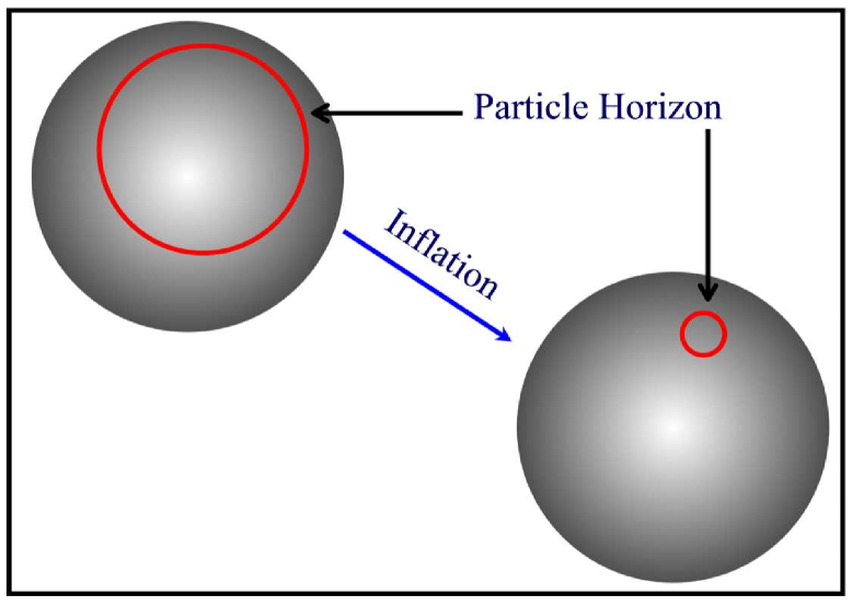
Figure 4: This figure illustrates the more natural perspective contrasted to that of Figure (3). The frame of reference is that of comoving coordinates, which puts the observer at rest relative to the expansion. In this frame the particle horizon is seen to shrink.

What does this mean? This implies that during a period of inflation the comoving frame (parameterized by $r,\theta,\mbox{and}\;\phi$), SHRINKS! Remember that the comoving coordinates represent the system of coordinates that are at rest with respect to the expansion. In other words, instead of viewing the spacetime as expanding it is equally valid to view the particle horizon as shrinking. To visualize this, it is perhaps useful to again consider the idea of an expanding balloon (see Figures 3 and 4). Normally, in this example, one views two points on the surface of the balloon as getting farther apart because the balloon is expanding. However, if one chooses a frame in which the surface is not expanding this would mean that the metric, or way of measuring, would shrink. Thus, the distance between the points would get larger, since the comoving coordinates got smaller. Each frame of reference has its advantages. For the remainder of this paper I will choose the frame where the universe is seen to expand. This has the advantage that the Hubble length remains ‘almost’ constant during inflation, which eases the discussion in the analysis to follow.

Notice it is now justified to use the flat universe approximation, since inflation forces $\Omega=1$ by the fact that $1/a^{2}H^{2}$ increases so rapidly compared to $k$ in Equation (49). Also note that $\Omega$ doesn’t have to be entirely matter dominated. For example, $\Omega=\Omega_{M}+\Omega_{\Lambda}=.3+.7=1$ is an acceptable configuration in the inflation scenario.

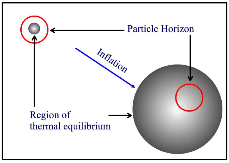
Figure 5: This figure illustrates that during inflation regions that have achieved thermal equilibrium can be expanded outside the particle horizon (Hubble distance). After inflation, the particle horizon begins to expand faster than the spacetime and these regions reenter the horizon. Inflation is the only known way to explain this uniformity, thus solving the horizon problem.

So, the picture during inflation is that the spacetime background expands at an accelerating pace. This resolves the horizon problem, since causal regions in the early universe are stretched to regions much larger than the Hubble distance. This is because during inflation the scale factor evolves at super-luminal speeds, whereas the particle horizon (Hubble distance) is approximately constant. The particle horizon does expand at the speed of light (by definition), but this pales in comparison to the evolution of the scale factor. Remember the Hubble distance is the farthest distance light could have traveled from a source to reach an observer. Once inflation ends, the scale factor returns to its sub-luminal evolution leaving the particle horizon to “catch up”. This situation is illustrated in Figure 5. So as we look out at the sky today we are still seeing the regions of uniformity that were stretched outside the particle horizon during inflation.

A more quantitative argument is given by considering the physical distance light can travel during inflation compared to after.

$$a(t_{rec})\int_{t_{inf}}^{t_{rec}}\frac{dt}{a(t)}\;\gg a(t_{0})\int_{t_{rec}}^{t_{0}}\frac{dt}{a(t)},$$ (50)

where $t_{inf}$ marks the beginning of inflation, $t_{rec}$ is the time of recombination, and $t_{0}$ is today.

Equation (50) can be understood by making the following estimates. In the first integral, the scale factor during inflation is given by, $a(t)\sim e^{Ht}$. Whereas, in the second integral one can assume the scale factor is primarily matter dominated $a(t)\sim t^{2/3}.$ Furthermore, the integral on the right can be simplified by taking $t_{rec}=0$. Of course this only increases the integral. Lastly, $t_{inf}$ can be set equal to zero and then $t_{rec}=\Delta t$ is the time inflation lasts. Thus,

$$e^{H\Delta t}\int_{0}^{\Delta t}\frac{dt}{e^{Ht}}\;\gg t_{0}^{2/3}\int_{0}^{t_{0}}\frac{dt}{t^{2/3}}.$$

Evaluating the integrals and a bit of algebra gives,

$$H^{-1}\Big{(}e^{H\Delta t}-1\Big{)}\;\gg 3t_{0}=2H^{-1},$$ (51)

where the last step uses $H=\dot{a}/a=2/3t$. So, we can see from (51) that as long as inflation lasts long enough ($\Delta t$) then the horizon problem is solved.

With the discussion presented thus far, the monopole problem is solved trivially. The number of predicted monopoles per particle horizon at the onset of inflation is on the order of one (300years, ). As discussed previously, this would result in a density today that would force $\Omega\gg 1$, which is not observed. As stated previously, the comoving (causal) horizon shrinks during inflation. Thus, if the universe starts with one monopole, it may contain that one monopole after inflation, but no more. However, this is highly unlikely if the universe inflates by an appreciative amount. Furthermore, inflation redshifts all energy densities. So, as long as the temperature does not go near the critical temperature after inflation, no additional monopoles may form.

This holds true for the other topological defects and unwanted relics associated with spontaneous symmetry breaking (SSB) in unified theories. This leads one to ask, why would the temperature increase after inflation? The mechanism by which this reheating of the universe takes place is related to the mechanisms that bring about the demise of the inflationary period. These mechanisms are understood through the dynamics of scalar fields, to be discussed in the next section.

One question has been left unresolved with reference to the problems of initial values in the hot Big Bang model. This is the problem of the origin of structure in the universe. It was pointed out that the DeSitter universe is left empty and cold with no stars or galaxies. The flatness and monopole problem were resolved by a redshifting of the various energy densities. But, if no energy is present, how can particle creation take place? This peculiar feature of inflation will be discussed in the next section, but here I would like to present a qualitative description.

At the end of inflation, all energy densities have become negligible except the vacuum density (or cosmological constant if you prefer). Where did the energy go? It went into the gravitational ‘potential’ of the universe, so energy is still conserved (guthp1, ),(guthp2, ),. Thus, at the end of inflation there is a universe filled with vacuum energy, which takes the form of a scalar field. This scalar field is coupled to gauge fields, such as the photon. As the scalar field releases its energy to the coupled field, the universe goes through a reheating phase where particles are created as in the hot Big Bang model. The energy for this particle creation is provided by the ‘latent’ heat locked in the scalar field. More will be said on this later, but the important point is that the hot Big Bang model picks up where inflation leaves off. Thus, one may be inclined to say, inflation is a slight modification to the hot Big Bang model. One author refers to inflation as, “a bolt on accessory” (liddleeprint, ).

This all sounds very appealing, however reheating is a fragile topic for inflation and results in a number of different models. This derives from the fact that if the temperature is too high at the time of reheating, the unwanted particle relics could be re-introduced into the model! As a result, many different reheating scenarios have been proposed, along with many different models for the onset of inflation.

One surprise from inflation makes all of this worry worth it. Along with offering a solution to the various initial value problems of the hot Big Bang, inflation offers a mechanism to seed the large-scale structure of the universe. Depending on the model chosen, (e.g., reheating temperature, onset conditions, etc.) one gets predictions for the large-scale structure of the universe and the anisotropies in the cosmic background. As will be seen in the next section, this again demonstrates how the very small (quantum mechanics) can impact the very large (universal structure). In some models of inflation, a small fluctuation in the quantum foam of the Planck epoch ($t<10^{-43}$) can give rise to the formation of galaxies, solar systems, and eventually human life! We are the result of pure chance! This is getting a little ahead of the game, so let us consider a quantitative and mechanical explanation of inflation.

V.3 Inflation and Scalar Fields

As stated above, inflation is capable of solving many of the initial value, or ‘fine-tuning’, problems of the hot Big Bang model. This is assuming that there is some mechanism to bring about the negative pressure state needed for quasi-exponential growth of the scale factor. In the early 1980’s, Alan Guth (guth, ) was studying properties of grand unified theories or GUTs. It was found in the late 70’s that these theories predict a large number of topological defects (Lindecor1, ),(Lindecor2, ). Guth was specifically addressing the issue of monopole creation in the SU(5) GUT. It was found that the theory predicts a large number of these monopoles, and that they should ‘over-close’ the universe (Lindecor1, ),(Lindecor2, ). This means that the monopole contribution to $\Omega$ is greater than the observed upper-bound on the density parameter, $\Omega>4$, which comes from observation (turner, ). To remedy this, Guth suggested that the symmetry breaking associated with scalar fields in the particle theory cause the universe to enter a period of rapid expansion. This expansion ‘dilutes’ the density of the monopoles created, as stated above.

The first step in understanding the dynamics of scalar fields is to undertake the study of field theory. In field theory, one considers a Lagrangian density, as opposed to the usual Lagrangian from classical mechanics. This is because the scalar field is taken to be a continuous field, whereas the Lagrangian in mechanics is usually based on discrete particle systems. The Lagrangian ($L$) is related to the Lagrangian density ($\mathcal{L}$) by,

$$L=\int\mathcal{L}\;d^{3}x.$$ (52)

Usually the scalar field is represented by a continuous function, $\phi(x,t)$, which can be real or complex. Given a potential density of the field, $V(\phi)$, $\mathcal{L}$ takes the form,

$$\mathcal{L}=\frac{1}{2}\partial_{\mu}\phi\partial^{\mu}{\phi}-V(\phi).$$ (53)

The resulting Euler-Lagrange equations result from varying the action with respect to spacetime (ryder, ),

$$\frac{\partial{\mathcal{L}}}{\partial{\phi}}-\frac{d}{dx^{\mu}}\Bigg{(}\frac{\partial{\mathcal{L}}}{\partial{(\partial_{\mu}{\phi})}}\Bigg{)}=0,$$ (54)

where $x^{\mu}=(t,-x^{i})$ as usual, and $\hbar=c=1$. Also note, $g_{\mu\nu}=\mbox{diag}(1,-1,-1,-1)$, the factor of $\sqrt{-g}$ that usually appears in the action and other equations involving tensor densities will be $\sqrt{-(-1)}=1$ (Minkowski space). The resulting equation is

$$\ddot{\phi}+3H\dot{\phi}=-V^{\prime}(\phi).$$ (55)

The prime represents differentiation with respect to $\phi$ and the term containing the Hubble constant serves as a kind of friction term resulting from the expansion. The field is taken to be homogeneous, which eliminates any gradient contributions. This homogeneity is a safe assumption, since physical gradients are related to comoving gradients by the scale factor,

$$\nabla_{{physical}}=a^{-1}(t)\nabla_{{comoving}}.$$ (56)

Thus, the inhomogeneities in the field are redshifted away during inflation since the scale factor increases by a large amount.

One can also define the stress-energy tensor by use of Noether’s theorem (ryder, ),

$$T^{\mu\nu}=\partial^{\mu}\phi\partial^{\nu}\phi-g^{\mu\nu}\mathcal{L}.$$ (57)

This is useful, because it can be compared to $T^{\mu\nu}$ for a perfect fluid, namely,

$$T^{\mu\nu}=\mbox{diag}(\rho,p,p,p).$$

Using (53) in (57) yields,

$$\rho=T^{00}=\frac{1}{2}\dot{\phi}^{2}+V(\phi)+\frac{1}{2}(\nabla\phi)^{2}.$$

The calculation for the pressure is a bit more subtle,

$$p=(T^{11}+T^{22}+T^{33})/3.$$

Consider the first component of pressure, again making use of (53) and (57),

$$T^{11}=\partial^{1}\phi\partial^{1}\phi-g^{11}\Bigg{[}\frac{1}{2}\partial_{\beta}\phi\partial^{\beta}\phi-V(\phi)\Bigg{]}.$$

Since $g^{11}=-1$ and one can use the metric to raise and lower indices,

$$T^{11}=(\partial^{1}\phi)^{2}-V(\phi)+\Bigg{[}\frac{1}{2}g^{\beta\gamma}\partial_{\beta}\phi\partial_{\gamma}\phi\Bigg{]}.$$

Since the metric is diagonal this yields,

$$T^{11}=(\partial^{1}\phi)^{2}-V(\phi)+\frac{1}{2}\Bigg{[}g^{00}\partial_{0}\phi\partial_{0}\phi+g^{11}\partial_{1}\phi\partial_{1}\phi+g^{22}\partial_{2}\phi\partial_{2}\phi+g^{33}\partial_{3}\phi\partial_{3}\phi\Bigg{]},$$

$$=(\partial^{1}\phi)^{2}-V(\phi)+\frac{1}{2}\dot{\phi}^{2}-\frac{1}{2}(\nabla{\phi})^{2}.$$

Similarly, the $T^{22}$ and $T^{33}$ components may be found. So for the total pressure one finds,

$$p=\frac{1}{3}\sum_{i}T^{ii},$$

or,

$$p=\frac{1}{2}\dot{\phi}^{2}-V(\phi)-\frac{1}{6}(\nabla\phi)^{2}.$$ (58)

From the $T^{00}$ component we already found,

$$\rho=\frac{1}{2}\dot{\phi}^{2}+V(\phi)+\frac{1}{2}(\nabla\phi)^{2}.$$ (59)

Equations (58),(59) for the pressure and the energy density, show that the equation, $p=-\rho$ is not quite satisfied. A first resolution to this problem is to again assume that the scalar field ($\phi$) is spatially homogeneous, allowing one to eliminate the gradient terms ($\nabla\phi$). This assumption is only made at this point to simplify the analysis. As we have seen if one keeps the terms, it can be shown that the gradients are redshifted away by the expansion (56). Ignoring gradients, the equations become

$$p=\frac{1}{2}\dot{\phi}^{2}-V(\phi),$$ (60)

$$\rho=\frac{1}{2}\dot{\phi}^{2}+V(\phi).$$ (61)

The first term $\frac{1}{2}\dot{\phi}^{2}$ can be thought of as the kinetic energy and the second as the potential, or configuration energy. It is now possible to explicitly see where Equation (55) came from if we assume the field can be described as a ‘perfect’ fluid. This assumption allows us to use a continuity equation,

$$\dot{\rho}+3H(\rho+p)=0.$$ (62)

By plugging in the energy density of the field (61) and making use of the Friedmann equation (to get $H$) one obtains Equation (55) in perhaps a more enlightening way.

From the pressure and energy density derived above, we see that the requirement that $p=-\rho$ can be approximately met, if one requires $\dot{\phi}\ll V(\phi)$. This leads to what is called the slow-roll approximation (SRA), which provides a natural condition for inflation to occur. To assure the constraint on $\dot{\phi}$, one must also require that $\ddot{\phi}$ be negligible. Given these requirements, we will to define the slow-roll parameters and introduce the Planck mass  (liddle3, ),

$$\epsilon(\phi)=\frac{M^{2}_{p}}{16\pi}\Bigg{(}\frac{V^{\prime}}{V}\Bigg{)}^{2},$$ (63)

$$\eta(\phi)=\frac{M^{2}_{p}}{8\pi}\Bigg{(}\frac{V^{\prime\prime}}{V}\Bigg{)}.$$ (64)

At this point, it is useful to distinguish $\phi$ as the inflaton field. Inflaton is the name given to $\phi$, since its origin does not have to originate with a specified particle theory. Although the original hope was that $\phi$ would help determine the correct particle physics models, current model building does not necessarily require specific particle phenomenology. This is actually an advantage for inflation, it retains its power to solve the initial value problems, yet it could arise from any arbitrary source (i.e., any arbitrary inflaton).

However, observation of the large-scale structure of the universe and anisotropies in the cosmic background should be able to constrain the inflaton parameters to a particular region. This can then be used by particle theorists, as a motivation for some required scalar field. Observational aspects of inflation will be considered in the next section, but this property of the inflaton field manifests itself as one of the greatest contributions of cosmology commensurate with particle theory. Some examples of potentials that have been proposed for the inflaton are presented below (veneziano, ),(liddleeprint, ).

$$V(\phi)=\lambda(\phi^{2}-M^{2})^{2}\quad$$ Higgs potential (65)

$$V(\phi)=\frac{1}{2}m^{2}\phi^{2}$$ Massive scalar field (66)

$$V(\phi)=\lambda\phi^{4}$$ Self-interacting scalar field (67)

$$V(\phi)=2H_{i}^{2}\Big{(}3-\frac{1}{s}\Big{)}e^{-\phi/\sqrt{s}}\quad\quad$$ Dilaton scalar field (string theory) (68)

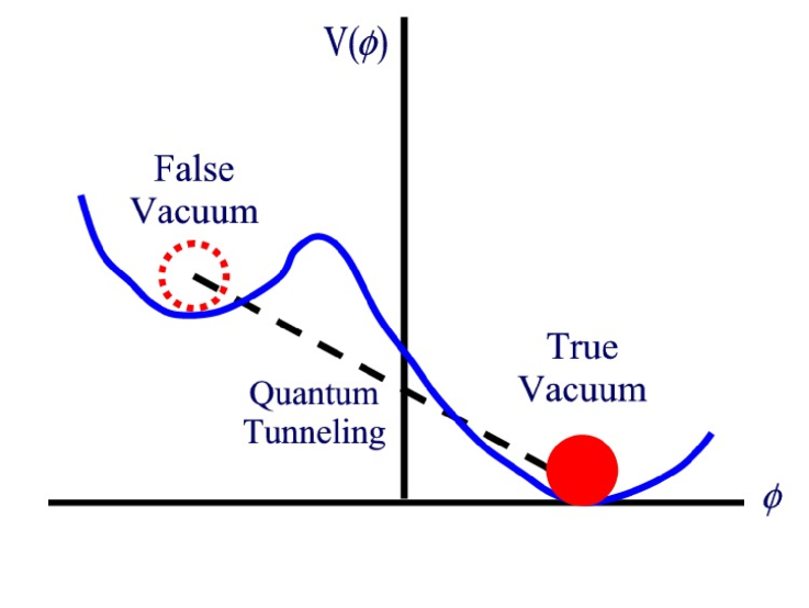
Figure 7: Toy Model For Original Inflaton

In Guth’s original inflation scenario (guth, ), the inflaton field ($\phi$) sits at a local minimum and is trapped in a false vacuum state (see Figure 7). The vacuum state of a field or particle is the lowest energy state available to the system. Some examples are the ground state of the hydrogen atom (-13.6 eV) and the ground state of the harmonic oscillator ($\frac{1}{2}\hbar\omega$). The concept of ‘false’ vacuum comes from examination of Figure 7. If $\phi$ is ‘placed’ in the potential well on the left, the lowest energy available is that of the false vacuum. The only way $\phi$ can get out of this local minimum is by quantum tunneling, after some characteristic time. As tunneling takes place the universe inflates. Inflation halts when $\phi$ reaches the false vacuum and bubbles of the false vacuum coalesce releasing the ‘latent’ heat that was stored in the field. This is much like the way bubble nucleation occurs when opening a bottle of compressed liquid (like soda). Energy escapes from the soda in the form of carbon dioxide and the liquid enters a lower more favorable energy state.

Tunneling that leads to bubble nucleation is a first order phase transition. This is very similar to processes that take place in the study of condensed matter physics, fluid dynamics, and ferromagnetism (see for example (maris, ) and (kittel, )). The bubbles experience a state of negative pressure. Once created, they continue to expand at an exponential rate. Each expanding bubble corresponds to an expanding domain. However, when one carefully investigates this situation, one finds that the bubbles can collide as they reach the false vacuum. Furthermore, the size of these bubbles expands at too great of a rate and the corresponding universe is left void of structure. One finds that too much inflation occurs and the visible universe is left empty. This is referred to as the ‘graceful exit’ problem. Again one is presented with an empty universe, which was the same reason that the DeSitter universe idea was abandoned.

Guth and others further tried to remedy these problems by fine-tuning the bubble formation. The problem with this is two fold. One, cosmologists and particle theorists don’t like fine-tuning. The idea is to form a model that gives our universe as a usual result that follows from natural consequences. By natural one means that the scales of the model are related to the fundamental constants of nature; e.g., quantum gravity should occur at the Planck scale, since this scale is the only one natural in units (c,$\hbar$,G). Secondly, if the model is fine-tuned to agree with the observations of the anisotropies in the cosmic background, the bubbles would collide far too often. This results in the appearance of topological defects, like the monopoles. However, this was the whole reason inflation was invoked in the first place.

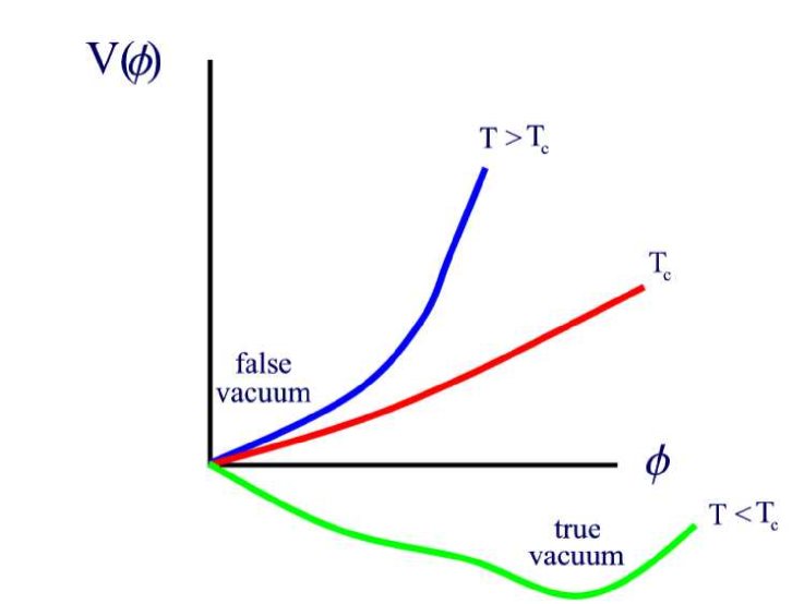
Figure 8: Toy Model For New Inflation – When the temperature of the universe decreases to the critical temperature $T_{c}$, the scalar field potential experiences a second order phase transition. This makes the ‘true’ vacuum state available to $\phi$.

In 1982, a solution to the graceful exit problem was proposed by Linde (linde6, ) and independently by Steinhardt and Albrecht (steinhardt7, ). This New Inflation model solves the graceful exit problem by assuming the inflaton field evolves very slowly from its initial state, while undergoing a phase transition of second order. Figure 8 illustrates this by again considering the evolution of $\phi$. If $\phi$ ‘rolls’ down the potential at a slow rate, one obtains the amount of inflation needed to solve the initial value problems. After the universe cools to a critical temperature, $T_{c}$, $\phi$ can proceed to its ‘true’ vacuum state energy. The transition of the potential is a second order phase transition, so this model does not require tunneling (300years, ). This type of transition is similar to the transitions that occur in ferromagnetic systems (kittel, ).

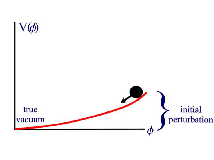
Figure 9: Toy Model For Chaotic Inflation – The inflaton finds itself displaced from the true vacuum and proceeds to ‘roll’ back. Inflation takes place while the inflaton is displaced.

The majority of current models rely on another concept coined by Linde as Chaotic Inflation (lindecor3, ). This model differs from Old and New Inflation in that no phase transitions occur. In this scenario the inflaton is displaced from its true vacuum state by some arbitrary mechanism, perhaps quantum or thermal fluctuations. Given this initial state, the inflaton slowly rolls down the potential returning to the true vacuum (see Figure 9). This model has the advantage that no fine-tuning of critical temperature is required. This model presents a scenario, which can be fulfilled by a number of different models.

After the displacement of the inflaton, the universe undergoes inflation as the inflaton rolls back down the potential. Once the inflaton returns to its vacuum (true) state, the universe is reheated by the inflaton coupling to other matter fields. After reheating, the evolution of the universe proceeds in agreement with the Standard Big Bang model.

Although the inflaton could in principle be displaced by a very large amount, all the inflationist need be concerned with is the last moments of the evolution. This is when the perturbations in the scalar field are created that eventually lead to large-scale structure and anisotropies in the cosmic background. As long as the inflaton is displaced by a minimal amount (minimal to be defined in a moment) the initial value problems will be solved. When considering quantum fluctuations resulting in the displacement of $\phi$, minimal displacement is easily achieved.

Successful evolution is only possible if $V(\phi)$ is very flat and has minimal curvature. In terms of (63) and (64) this suggests that inflation will occur as long as the SRA requirements hold.

$$\epsilon\ll 1,\;\;\;\;\;\;\;|\eta|\ll 1.$$ (69)

This method is successfully used in a number of inflationary models that make predictions in accordance with observation. It must be stated again that Chaotic Inflation results in a very general theory. The inflaton field originally proposed by Guth’s model was that of a grand unified theory, but within the Chaotic Inflationary scenario any inflaton field can be used that satisfies the SRA. With these general requirements, potentials used in supergravity, superstrings, and supersymmetry theories can be used to motivate inflation.

Using the energy density obtained in equation (61) one can restate the Friedmann equation (45) in terms of the scalar field.

$$H^{2}=\frac{8\pi G}{3}\Bigg{[}V(\phi)+\frac{1}{2}\dot{\phi}^{2}\Bigg{]},$$ (70)

Also, the equations of motion derived in (55) are restated here for convenience.

$$\ddot{\phi}+3H\dot{\phi}=-V^{\prime}(\phi).$$ (71)

Using the SRA, one can simplify these equations by eliminating the $\dot{\phi}^{2}$ and $\ddot{\phi}$ terms. This leaves the more tractable equations shown below, which remain valid until $\phi$ approaches the true vacuum; i.e., $\epsilon\sim 1$.

$$H^{2}=\frac{8\pi V(\phi)}{3M_{p}^{2}},$$ (72)

$$3H\dot{\phi}=-V^{\prime}(\phi),$$ (73)

where $M_{p}$ is the Planck mass and has been substituted for $G$,

$$M_{p}\equiv 1/\sqrt{G},$$

remembering that $\hbar=c=1$.

One can use equations (72) and (73) to manifest the connection between the slow-roll condition (69) and the generic definition of inflation, that is $\ddot{a}>0$. First note that

$$H=\frac{\dot{a}}{{a}}\Rightarrow\;\dot{H}=\frac{\ddot{a}}{a}-\Big{(}\frac{\dot{a}}{a}\Big{)}^{2}.$$

For inflation to take place means $\ddot{a}(t)>0$ and $a(t)$ is always positive thus,

$$\frac{\ddot{a}}{a}>0\Rightarrow\;\dot{H}+H^{2}>0,$$

$$\Leftrightarrow-\frac{\dot{H}}{H^{2}}<1.$$ (74)

Using (72) and differentiating with respect to time,

$$2H\dot{H}=\frac{8\pi}{3M^{2}_{p}}\frac{d\phi}{dt}\frac{d}{d\phi}\Big{(}V(\phi)\Big{)},$$

$$\Rightarrow\dot{H}=\frac{8\pi\dot{\phi}V^{\prime}}{6M^{2}_{p}H}.$$

Plugging this result into (74) gives,

$$-\frac{\dot{H}}{H^{2}}=-\frac{\dot{\phi}V^{\prime}}{2HV}<1.$$

Solving (73) for $\dot{\phi}$ and plugging the result into the last equation, we obtain

$$\dot{\phi}=-\frac{V^{\prime}}{3H},$$

$$-\frac{\dot{H}}{H^{2}}=\frac{(V^{\prime})^{2}}{6H^{2}V}<1.$$

Lastly, substituting $H^{2}$ from (72) one obtains,

$$-\frac{\dot{H}}{H^{2}}=\frac{M^{2}_{p}}{16\pi}\Big{(}\frac{V^{\prime}}{V}\Big{)}^{2}<1.$$ (75)

But this is just the slow-roll condition $\epsilon\ll 1$. So again one is reminded that inflation will take place until $\epsilon\sim 1$, which has been shown to be equivalent to $\ddot{a}>0$.

V.3.1 Modeling the Inflaton Field

The equations of motion derived above (72),(73) describe the evolution of an arbitrary potential $V(\phi)$ subject only to the constraint that $V(\phi)$ conform to the slow roll conditions away from its minimum. As mentioned previously, the conditions for inflation are arbitrary and inflation will occur as long as $\ddot{a}>0$. There are three cases that are of particular interest (peacock, ).

• Polynomial Inflation. $V(\phi)\propto\phi^{n}$. This gives a scale factor which behaves quasi-exponentially.

  $$a(t)\sim\exp\Bigg{(}\phi^{n/2}kt\Bigg{)}\;\;\;\;\mbox{where}\;\;k=\sqrt{\frac{8\pi}{3M_{p}^{2}}}.$$

  For particle theorist $n=2,4$ are most favorable, since they describe renormalizable particle theories (ryder, ).

• Power-law Inflation. $V(\phi)\sim\exp\Big{(}-\sqrt{\frac{16\pi}{n}}\;\frac{\phi}{M_{p}}\Big{)}$. This gives $a(t)\sim t^{n}$. The only requirement being that $n>1$.

• Intermediate Inflation. $V(\phi)\sim\phi^{\mathcal{F}}$, where $\mathcal{F}=4(n^{-1}-1)$. This yields $a(t)\sim e^{(t/t_{0})^{n}}.$

As an example consider a simple polynomial model with $n=2$.

$$V(\phi)=\frac{1}{2}m^{2}\phi^{2},$$

$$V^{\prime}(\phi)=m^{2}\phi,$$

$$V^{\prime\prime}(\phi)=m^{2}.$$

The slow roll condition $\epsilon<1$ implies

$$\epsilon=\frac{M^{2}_{p}}{16\pi}\Bigg{(}\frac{V^{\prime}}{V}\Bigg{)}^{2}=\frac{M^{2}_{p}}{16\pi}\Bigg{(}\frac{m^{2}\phi}{\frac{1}{2}m^{2}\phi^{2}}\Bigg{)}^{2}<1,$$

$$\Longrightarrow\phi>M_{p}.$$

In other words, the inflaton field must be larger than the Planck energy. This is actually the value one would expect for the cosmological constant, since the only natural scale at high energy is the Planck scale. However, inflation (as it has been presented) relies on the evolution of a classical field. If the value of the field is in the quantum regime, where the Planck scale lives, inflation can not be treated classically. Fortunately, there are many resolutions to this problem. First, what really matters in the field equations is the potential energy density of the field; namely,

$$V(\phi)=\frac{1}{2}m^{2}\phi^{2}.$$

Remember that $V$ appeared in the Lagrangian density, thus $V$ is actually a density. From this equation one can see that the magnitude of the potential, and, therefore, the energy scale of the theory, depend on ‘$m$’ as well as $\phi$. ‘$m$’ represents the mass of the inflaton and one resolution to the high value of $\phi$ is to introduce a small mass for the inflaton; i.e., make ‘$m$’ small.

Another resolution to this scale problem is to limit considerations to the final part of the evolution of the inflaton. As stated before, the inflaton evolves until $\epsilon=1$ when the inflaton then reheats the universe. The most important consequences of inflation are its resolution of the initial value problems and its predictions about large-scale structure and the cosmic background anisotropies. As we will see most of these phenomena only require analysis of the last moments of ‘e-foldings’ of inflation. E-folding is a way of measuring how the scale factor increases. Since,

$$a=a_{0}\exp(H\Delta t),$$

one e-folding is defined as the amount of time for $a$ to grow by a factor of $e$:

$$\Delta t=H^{-1}.$$

It will be shown that only 60 e-foldings are needed to resolve the initial value problems and the scales that are important in determining structure in the universe only depend on modes that are present during these last 60 e-foldings.

However, it must be pointed out that many people find problems with these conditions on $\phi$. The idea of fine-tuning the mass of the inflaton ‘$m$’ is certainly unappealing. One of the appealing aspects of inflation was its resolution of the initial value or fine-tuning problems of the Big Bang model. But, now we are again confronted with an initial value problem. This problem can be resolved by addressing inflation in the context of a quantum gravity theory such as superstring theory. I will not pursue such issues in this paper, although the reader is again referred to the eprint archive for recent efforts.

V.3.2 The Amount of Inflation

One can find the amount of inflation by considering the change of the scale factor. Considering the example of quasi-exponential expansion, meaning that the Hubble constant need not be constant. Then,

$$\displaystyle{a(t)=a_{0}\exp{(Ht)}}$$ (76)

$$\displaystyle{\Rightarrow\ln\Bigg{(}\frac{a(t)}{a_{0}}\Bigg{)}=Ht},$$

$$\mathcal{N}\displaystyle{\equiv\ln\Bigg{(}\frac{a(t_{final})}{a(t_{initial})}\Bigg{)}=\int_{t_{i}}^{t_{f}}Hdt\quad\quad}$$ Number of e-foldings

Using the slow-roll equations, the number of e-foldings can be expressed in terms of the inflaton potential. Dividing (73) by (72) yields,

$$\frac{3\dot{\phi}}{H}=\frac{3H\dot{\phi}}{H^{2}}=-\frac{V^{\prime}}{8\pi V}\Big{(}3M^{2}_{p}\Big{)},$$

$${\Rightarrow\frac{\dot{\phi}}{H}=-\frac{M^{2}_{p}}{8\pi}\Bigg{(}\frac{V^{\prime}}{V}\Bigg{)}}$$

Using this result, with the formula for $\mathcal{N}$ (76), one gets,

$$\mathcal{N}=\int_{t_{i}}^{t_{f}}Hdt=\int_{t_{i}}^{t_{f}}H\frac{dt}{d\phi}\>d\phi=\int_{t_{i}}^{t_{f}}\frac{H}{\dot{\phi}}\>d\phi=-\frac{8\pi}{M^{2}_{p}}\int_{\phi_{i}}^{\phi_{f}}\frac{V}{V^{\prime}}\>d\phi.$$

$$\mathcal{N}\simeq\frac{8\pi}{M^{2}_{p}}\int_{\phi_{f}}^{\phi_{i}}\frac{V}{V^{\prime}}\>d\phi.$$ (78)

Here the fact that the SRA has been used is expressed using ‘$\simeq$’ in (78).

For $\mathcal{N}>60$, which is needed to solve the initial value problems (peacock, ), we again find $\phi\gg M_{p}$. This can be seen from (78), where $V^{\prime}\sim V/\phi$ using the SRA. This means that if one chooses a potential of $\frac{1}{2}m^{2}\phi^{2}$, one must choose the coupling, $m^{2}$ to be small. Given a self interacting potential term, $\lambda\phi^{4}$, the coupling must be extremely weak, $\lambda\ll 1$. This coupling agrees nicely with theories of supergravity and certain string theories, although other potentials are ruled out because of their couplings, such as the weak coupling. This leaves the question. Can inflation be considered without a theory of quantum gravity? As mentioned before, the inflationist is often not concerned with these initial stages of inflation. The common standpoint is that chaotic inflation can present an evolution and then one studies the predictions of this evolution. As aesthetically displeasing as this may be, it allows cosmology to progress further without a quantum theory of gravity. Ultimately this issue will be addressed within the context of a theory of quantum gravity to create a complete picture of the creation of the universe. However, it has been argued that a complete understanding of the universe may be avoided in a scenario known as eternal inflation (Lindecor4, ),(guthp2, , and references within ),(guthp1, , and references within). Time does not permit to discuss these models in detail, however for a popular account (Lindecor5, ) is an excellent starting point.

Given the slow-roll conditions and the number of required e-foldings ($\mathcal{N}$), one can test a model inflaton to see if it is compatible with an inflationary scenario. With this generic framework that has been set forth, one can construct particle theories and then test their validity within the context of inflation theory. However, the slow-roll approximation and initial value problems ($\mathcal{N}>60$) are not the only constraints on the inflaton and therefore particle theory. The inflaton is further restricted by the predicted large-scale structure of the universe, along with the mechanisms involved with reheating of the universe at the end of inflation. The large-scale structure is determined by density perturbations resulting from quantum fluctuations in the evolution of the inflaton field. This analysis can actually be done without the advent of quantum gravity; however, it is outside the scope of this paper. Instead, the author hopes to manifest the stringency of these parameters on the inflaton field by addressing the observational consequences and predictions that inflation offers. In the next section these observational tests will be explored.

VI Observational Tests of Inflation

It was shown in the last section that if the number of e-foldings exceeds $60$, then inflation can solve the horizon, flatness, and relic (monopole) problems. One generally favors this model over a Big-Bang model, because of its naturalness. That is to say, inflation offers a generic scenario for solving the initial value problems. However, this arbitrariness can also be viewed as a problem for inflation. For instance, throughout this paper it has been assumed that inflation necessarily leads to a flat universe ($k=0$). However, Hawking, Turok, Linde, and others have shown that inflation can result in a non-flat universe (open1, ),(open2, ). Models can be created that produce unwanted or wanted relics and contain inhomogeneities. Furthermore, we have seen inflation requires an inflaton field to drive the inflation. Where does it come from and what is its natural value? Originally Guth had the inflaton as corresponding to a GUT transition; however, today the preferred energy range is on the order of the Planck scale. Thus, to fully understand inflation one needs a full quantum theory of gravity. For these reasons one may ask; Is inflation a particular type of cosmological model, or is inflation an arbitrary constituent of any successful theory of the cosmos?

Inflation’s strength today can be seen from its predictions of large-scale structure. Different models predict different structure and this can be used to narrow the number of possible models. One can further constrain the inflationary models by cosmological parameters. The cosmic background observations, galaxy surveys, lensing experiments, and standard candles can be used pin-down the cosmological parameters. In this way, observational parameters (e.g., $H$, $\Omega_{M}$,$\Omega_{\Lambda}$) can be given viable ranges and inflationary parameters can be determined based on these preferred ranges. With the cosmological parameters determined, inflation parameters depend only on the height and shape of the inflaton potential. The inflaton potential correspondingly yields predictions about the large-scale structure of the universe and the anisotropies in the cosmic background radiation.

The study of large-scale structure has been pursued for many years (zeldovich, ). The problem was that there was an appealing mechanism which could produce the types of perturbations needed to produce the observed large-scale structure. These perturbation types are manifested by the anisotropies in the cosmic background. The anisotropies result from acoustic oscillations in the baryon-photon fluid just before recombination. Therefore, the anisotropy spectrum offers a ‘snap-shot’ of the seeded inhomogeneities that eventually resulted in galactic structure. These inhomogeneities were first discovered when COBE mapped the cosmic background in the early 1990’s (smoot, ). In this intimate way, the cosmic background and galaxy surveys predict a scheme by which structure was formed. The type of perturbation that is needed only results from models which predict Gaussian, adiabatic, nearly scale-invariant perturbations (carroll42, ). The only known models that fall into this category are the inflationary models (guth, ),(linde6, ),(steinhardt7, ).

VI.1 Perturbations and Large-Scale Structure

During the inflation epoch, perturbations (small fluctuations) of two types are generated: scalar (density) perturbations, and tensor (metric) perturbations. The scalar perturbations come from quantum fluctuations of the inflaton field before and during its evolution. Tensor perturbations arise from quantum fluctuations in the space-time metric within the quasi-DeSitter spacetime. Fluctuations of this type are a natural consequence of a DeSitter spacetime.

In DeSitter space there exists an event horizon. Consider the distance light can travel in comoving coordinates, which is given by (6) and $a(t)\sim\exp(Ht)$.

$$r=\int_{0}^{\infty}\frac{c\;dt}{a(t)}=\int_{0}^{\infty}\exp(-Ht)c\;dt=c/H.$$ (79)

The presence of this event horizon suggests the presence of thermal fluctuations in the fields, similar to those present in a black hole. This can be understood by appealing to the uncertainty principle. The event horizon causes the ground state modes of any fields present to be restricted in spatial extent. The uncertainty principle then requires, $\triangle p\geq\hbar H/c$, since the characteristic size is just $c/H$. This uncertainty in momentum gives rise to energy fluctuations and the corresponding Hawking temperature is given by (peacock, ),

$$kT_{DeSitter}=\frac{H}{2\pi},$$ (80)

where $k$ is the Boltzman constant relating the energy to the temperature.

This result provides a motivation for the existence of fluctuations in the metric and scalar field. As these perturbations are created during inflation they are inflated outside of the causal horizon (particle horizon). As mentioned in the previous section, the causal horizon is nearly stationary during inflation. Once the perturbation has been inflated outside the horizon, its ends are no longer in causal contact. In this way, the perturbations become ‘frozen-in’ as classical perturbations.

Ignoring the nonlinear, or super-horizon, effects of these perturbations may trouble the reader. However, as we shall see, ignoring these effects appears to be in agreement with the cosmic background data (hu2, ), (hu3, ), (hu4, ). As stated, one reason for choosing to ignore super-horizon evolution is the causal separation of the ends of the perturbation. However, this argument is far from rigorous and the study of nonlinear perturbations takes much care. Perturbation evolution relies on the extrinsic (super-horizon) properties of the spacetime manifold and is sensitive to the gauge of general relativity. The perturbation evolution can usually be ignored in regions where the pressure becomes negligible, which happens to be on the order of the horizon (peacock, ). This generally motivates one to ignore the super-horizon evolution, however for a complete treatment, see (branden, ),(ref31, ),(turner, , Chapter 8 and 9).

After inflation the expansion continues at sub-luminal speeds and these perturbations enter back inside the causal horizon. Thus, the most important perturbations for creating structure come from the ones that were exited near the end of the inflationary period (i.e., approximately the last 60 e-foldings). After the reheating process occurs, the inhomogeneities passing back inside the horizon cause fluctuations that seed the large-scale structure.

Pure exponential inflation, which corresponds to a DeSitter spacetime, has an interesting property. The spacetime is invariant under time translation. That is to say, there is no natural origin of time under true exponential expansion (peacock, , Chapter 11). The only fundamental size in the theory is that of the Hubble horizon ($c/H$). Thus, one expects that the amplitude of a ‘standing wave’ perturbation will be related to the horizon size, $c/H$, which is not changing. Therefore, we see why inflation predicts a scale-invariant spectrum for the perturbations.

This analysis can be illustrated through musical analogy. The fundamental mode of the perturbations are determined by the Hubble distance ($c/H$), much like the fundamental mode of a flute is determined by its length. Because the Hubble length (horizon) is nearly stationary during inflation, this means inflation predicts a scale-invariant, or Harrison-Zeldovich spectrum. Furthering this analogy, the ‘overtones‘ of the universe correspond to the inflaton potential that determines its behavior, much like overtones can be used to distinguish one instrument from another. However, as we have seen that inflation need not be exponential. The small deviations from DeSitter spacetime result in small deviations from a scale-invariant spectrum. These deviations can be used to successfully predict the correct potential for the inflaton.

The generated perturbations can be characterized by a power spectrum, $\delta_{H}^{2}(k)$. The $H$ indicates that the perturbation amplitude is taken to correspond to its value when it crossed the causal horizon. Quantitatively, this corresponds to $k=aH$, where $k$ is the wave number of the perturbation. Quantum field theory can be used to calculate an expression for $\delta_{H}$ similar to Equation (80) above (peacock, , Chapter 8).

$$\delta_{H}=\frac{H^{2}}{2\pi\dot{\phi}},$$ (81)

where $\phi$ is the inflaton. This formula manifests the connection between the inflaton potential and the perturbations generated during inflation.

One is generally interested in the scale dependence of the spectral index of these perturbations, since this dependence changes for different inflation models (lyth21, ).

$$n(k)-1\equiv 2\frac{d\delta_{H}}{d\ln{k}}.$$ (82)

For an absolute scale-invariant spectrum, it follows that $\delta$ is independent of $k$ and the above relation gives $n=1$ as one would expect. For a spectrum that is nearly scale-invariant the amount $n$ differs from one is referred to as the tilt of the spectrum. Although it is not at all obvious, (81) and (82) can be used along with the slow roll parameters (64),(63) to express the tilt as,

$$1-n=6\epsilon-2\eta.$$ (83)

The details of the calculation need not concern us here, for a derivation of this result see (dekel, ) or (peacock, ). This relation is only presented to demonstrate that the tilt, which is a discriminating factor between models, can be written in terms of the SRA parameters $\epsilon$ and $\eta$. Therefore, if an experimental consequence of the tilt is observable, one can find the appropriate values for the SRA and reconstruct the inflaton potential (lyth34, ).

VI.2 The Cosmic Background Anisotropies

The discovery of the anisotropies in the cosmic background by COBE created a new opportunity for verification of cosmological parameters and theories of large-scale formation. As discussed at the beginning of this paper, the CMB offers a ‘snap-shot’ of the universe at the time of recombination ($z\sim 1000$). The anisotropies that were present in the baryon-photon plasma at this time are manifested today by the temperature fluctuations in the spectrum. These fluctuations are representative of a nearly Gaussian, scale-invariant spectrum. As discussed previously, this is a unique prediction of inflation theories.

Although the quantitative details can become formible, the qualitative description of these temperature fluctuations is quite simple. During inflation, the perturbations formed must be of nearly the same amplitude and randomly distributed, as discussed above. After reheating takes place, these classical perturbations re-enter the horizon causing density fluctuations in the baryon-photon plasma. In over-dense regions, potential wells form that trap the plasma and cause it to heat up. At the same time, photon pressure induces a kind of restoring force to oppose the gravitational potential. In this way, a harmonic oscillator motion is set up in the plasma. These oscillations continue with no friction (viscosity) from the fluid. This is why they are referred to as adiabatic fluctuations. However, if this were not the case and the friction is deemed important, one obtains an isocurvature spectrum (huhuhu, ). These turn out to be indicative of cosmic strings, which are ruled-out by observation as a method of primordial structure formation. However, models containing cosmic strings that are produced during reheating following inflation may still play a major role in cosmological models (brandenberger, ).

At the time of recombination, when the photons were able to escape the fluid, they had to overcome the gravitational potentials. The picture is that the photons in these potential wells were hotter than the average, but this temperature difference was partially cancelled by the gravitational redshift resulting from the photons ‘climbing’ out of the potential well. This phenomena is know as the Sachs-Wolf effect. The result is that the photons that were in the wells have a slight temperature increase from those that were not. This variation is predicted by theory to be on the order of $10^{-5}$ (peacock, ). These oscillations propagate through the fluid at the speed of sound. Thus, there is a acoustic horizon that is generated within the surface of last scattering and if present today would have an angular size of about one degree on the sky.

One concern with the simplicity of this analysis is what effects, such as reionization in the surface of last scattering, must be considered? It is important to consider the mean free path of the photon as it travels within the fluid before escaping. This could affect the energy and therefore temperature of the spectrum. However, it turns out that this effect only appears on small angular scales within the spectrum and can be ignored (hu3, ). Also, any effects from CMB scattering off interstellar gas only appear in the spectrum at very small angles. These observations are of course useful, but offer little insight into examination of the early universe and formation of large-scale structure.

Given the predicted anisotropies from the Sachs-Wolf effect, the next step is to examine the cosmic background spectrum through observation. The anisotropies in the temperature of the cosmic background spectrum can be expanded in spherical harmonics (carroll42, ),

$$\frac{\Delta T}{T}=\sum_{lm}a_{lm}Y_{lm}(\theta,\phi),$$ (84)

The multipole coefficients are given by,

$$a_{lm}=\int dA\>Y^{*}_{lm}\frac{\Delta T}{T}.$$ (85)

The amount of anisotropy at multipole moment $l$ is expressed by the power spectrum,

$$C_{l}=|a_{lm}|^{2}.$$ (86)

The $C_{l}$’s measure the temperature anisotropy of two regions separated by angle $\theta$. This angle is related to the $l$’s by: $\theta\sim 180^{{}^{o}}/l.$ Thus, $l$ allows one to express the temperature variations of regions separated by an angle $180^{{}^{o}}/l$. The $l=0$ represents the monopole contribution to the anisotropy, which is of course zero (this is comparing a point separated from itself by $360^{{}^{o}}$. The next moment, $l=1$, is the dipole moment, which compares regions separated by $180^{{}^{o}}$. This anisotropy originates from our peculiar velocity, the motion of the Earth relative to the cosmic background. This moment is usually taken out of the spectrum to leave the ‘true’ anisotropy. The $l=2$ moment is the quadrupole contribution, which marks the first non-trivial anisotropy for understanding structure formation.

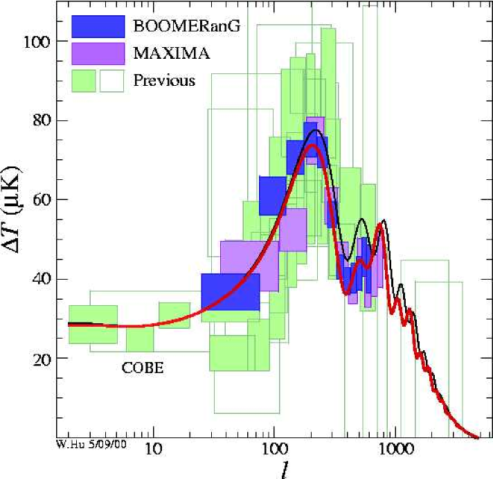
Figure 10: Power Spectrum Plot of the Cosmic Background – The data is normalized to the quadrupole ($l=2$) anisotropy detected by COBE. The Doppler peak corresponds to a maximum power fluctuation at a multipole of $l=220$, which is about an angle of one degree on the sky. This graph provided by Wayne Hu (huhuhu, ).

When the COBE data is plotted with multipole $l$ versus temperature variation, a peak is found to occur around $l=220$ or $1^{{}^{o}}$ (Figure (10)). This peak corresponds to the angular size on the sky of the acoustic horizon discussed before and has been called the Doppler peak. Thus, there is a maximum temperature variation at precisely the angle predicted by the Sachs-Wolf effect. Since a mechanism of this type can only be explained by an inflationary model, one is presented with a strong argument for inflation (huhuhu, ).

However, the peak is actually sensitive to the cosmological parameters, such as the Hubble constant and the curvature of the universe. If the universe is non-flat then the null geodesics are found to converge (diverge) in the case of spherical (hyperbolic) geometry. The angle subtended is given by $\theta_{H}\sim\Omega^{1/2}\>1^{{}^{o}}$. This means for the peak at $l=220$ we live in a universe which is flat. Although, this seems to represent a bit of circular logic. This difficulty can be remedied by calling upon other observational tests to constrain the parameters. These includ galaxy surveys, lensing experiments, or standard candle observations. When all of these methods are combined, strong constraints can be put on parameters and the best model can be determined.

The cosmic background is apparently richer in structure than was first realized. As we have discussed, inflation predicts fluctuations in both the scalar and tensor fields. This gives rise to slight differences in the anisotropies at small angles (large $l$). Also, there are multiple peaks in the spectrum following the peak at $l=220$ and the height and shape of the spectrum are related to the specifics of inflation models, such as the tilt.

To examine one aspect of the complexity involved, consider that the scalar and tensor perturbations can be fixed by their contribution to the quadrupole moment $C_{l=2}$ of the CMB (kamionkowski, ).

$$\mathcal{S}=6\>C^{scalar}_{l=2}=33.2\>[V^{3}/(V^{\prime})^{2}],$$ (87)

$$\mathcal{T}=6\>C^{tensor}_{l=2}=9.2V,$$ (88)

where $V=V(\phi)$ is the inflaton potential, $\mathcal{S}$ is the scalar contribution, and $\mathcal{T}$ is the tensor contribution. When the slow-roll approximation is considered and the determination of cosmological parameters is found by methods other than CMB analysis; e.g., for large-scale structure probing, one finds that the ratio $\mathcal{T/S}$ is less than order unity. This restricts $V\leq 5\times 10^{-12}$. Reformulating equation (82) in terms of the inflaton potential, one finds in Planckian units the relations for the scalar and tensor spectral indices, respectively.

$$1-n_{s}=\frac{1}{8\pi}\Bigg{(}\frac{V^{\prime}}{V}\Bigg{)}^{2}-\frac{1}{4\pi},$$ (89)

$$n_{t}=-\frac{1}{8\pi}\Bigg{(}\frac{V^{\prime}}{V}\Bigg{)}^{2}.$$ (90)

Although most models of inflation predict a near scale-invariant, or Harrison-Zel’dovich spectrum, the small deviations from differing potentials $V(\phi)$ give a way of testing inflation models. With future experiments such as MAP and PLANCK, these spectral indices will be found with great precision and the shape and height of the spectrum can be used to manifest the correct inflaton potential. In this way, inflation will be used to predict new particle physics, instead of the original scenario which was vice versa.

However, the ultimate test of inflation is the precise determination of the tensor perturbations, that is the $n_{t}$’s. This can’t be deduced from the CMB spectrum because both the scalar and tensor perturbations contribute to the temperature anisotropy. However, if a method could be devised to separate out the tensor perturbations and this spectrum were detected, it would be concrete evidence of an inflationary period. This is because inflation is the only way metric perturbations can survive to the present. This is due to the structure of a DeSitter spacetime.

The tensor spectrum can be separated by creating a polarization map of the CMB. The separation is then possible because the tensor perturbations have an intrinsic axial component, and the angular dependence can be determined from the metric. Whereas, the scalar perturbations have no dependence on direction. Therefore, the polarization vector can be constructed out of two parts, a curl and a gradient.

$$\vec{P}(\theta,\phi)=\vec{\nabla}A+\vec{\nabla}\times\vec{B},$$ (91)

where $\hat{n}$ gives the direction. Thus, to obtain the tensor terms one can take the divergence of this vector. Before proceeding further, it may be of interest to the reader why the perturbations only contain tensor and scalar contributions and vector type perturbations are absent. This is because massless vector fields are conformally invariant (turnertests, ). This invariance can be broken by introducing a mass term or by explicitly breaking the coupling. Although for a massive vector field the perturbations generated are far too small and die off far too quickly during the inflationary expansion (liddletests, ). Thus, a standard prediction of inflation is that there are no vector perturbations. But, isn’t the polarization a vector? No. The polarization is actually a $2\times 2$ trace free symmetric tensor. This tensor is written in terms of the Stokes parameters $Q(\hat{n})$ and $U(\hat{n})$, which give us the polarization in each direction. For an explanation of these parameters see, (jackson, , section 7.2).

$$\mathcal{P}_{ab}(\hat{n})=\frac{1}{2}\left(\begin{array}[]{cc}Q(\hat{n})&-U(\hat{n})\sin\theta\\ -U(\hat{n})\sin\theta&-Q(\hat{n})\sin^{2}\theta\\ \end{array}\right).$$ (92)

The polarization tensor can be expanded in tensor spherical harmonics (ref14, ),

$$\frac{\mathcal{P}_{ab}(\hat{n})}{T_{0}}=\sum_{lm}\Bigg{[}a^{G}_{(lm)}Y^{G}_{(lm)ab}(\hat{n})+a^{C}_{(lm)}Y^{C}_{(lm)ab}(\hat{n})\Bigg{]}$$ (93)

The $Y^{G}_{(lm)ab}$ and $Y^{C}_{(lm)ab}$ represent a basis for the gradient (scalar) and curl (tensor) perturbation terms in this polarization mapping. The $a^{G}_{(lm)}$’s and $a^{C}_{(lm)}$’s are again just found by exploiting the orthogonality. One can use this spectrum to construct necessary requirements for the potentials of the inflaton field and this analysis can therefore be used to distinguish the various inflation models.

VI.3 Summary

Scalar perturbations are the most easily detected form of perturbation. The scalar nature of these fluctuations arise from the fact that the perturbations are of mass fields in the primordial era, that is, before the time of decoupling. Different models of inflation and the corresponding reheating mechanisms differ in their predictions of mass variation. Regardless, these variations of the early universe eventually give rise to the structural formation of galaxy clusters, which can help distinguish the various theories of inflation and structure formation. Tensor perturbations are also detectable and these perturbations result from fluctuations in the space-time metric in the primordial era. Again, these perturbations are very small and would be very hard to detect. However, certain models of inflation predict wavelengths that could be detected by laser interferometry gravitational wave detectors, such as LIGO. If these waves were detected it would help eliminate many inflation models and help narrow the region of viable theories. Furthermore, inflation is the only theory that can currently account for a gravitational wave spectrum. The detection of the spectrum would be a great success for the inflation theory.

Both of these types of perturbations contribute to the $10^{-5}$ temperature fluctuation in the cosmic background. The biggest challenge for experimentalists is to separate the scalar and tensor contributions to the temperature fluctuations. In practice this is very difficult, if not impossible, and it becomes more practical to consider the polarization of the CBR.

For the inflationist, the goal of CRB measurements is to distinguish between the various models of inflation. A good way to begin, is to express many of the relations obtained thus far, in terms of $\epsilon$ and $\eta$. The number of e-foldings ($\mathcal{N}$) can be expressed in terms of $\epsilon$ using (63) and (78),

$$\mathcal{N}=\frac{2\sqrt{\pi}}{M_{p}}\int^{\phi_{f}}_{\phi_{i}}\frac{d\phi}{\sqrt{\epsilon}}.$$ (94)

Another useful relation, which may be found in the literature (ref31, ), gives a measure of when a given perturbations of wave length $k$ passes through the horizon and is therefore ‘frozen out’. This can be expressed as the number of e-foldings $\mathcal{N}(k)$ from the end of inflation.

$$\mathcal{N}(k)=62-\ln{\frac{k}{a_{0}H_{0}}}-\ln{\frac{10^{16}\>\text{GeV}}{V^{1/4}_{k}}}+\ln{\frac{V^{1/4}_{k}}{V_{e}^{1/4}}}-\frac{1}{3}\ln{\frac{V_{e}^{1/4}}{\rho^{1/4}_{RH}}}.$$ (95)

$V_{k}$ is the potential when the mode $k$ leaves the horizon, $V_{e}$ is the potential at the end of inflation, and $\rho_{RH}$ is the energy density after reheating. This expression may appear formidable, however it can be used to begin understanding density fluctuations. For example, the modes $k$ entering the horizon today, left the horizon at $\mathcal{N}(k)=50-70$. The uncertainty in this range manifests the lack of knowledge of the inflaton potential. Thus, once again different inflaton models make different predictions.

With the rapid advances in observational cosmology, cosmologists are able to use the abundance of data that is being obtained by the Hubble Space Telescope, balloon experiments, satellites (such as Chandra), etc. to narrow the parameters of the universe. Then with these values and the relations that have been presented in this section, one can use inflation to predict new physics for the pre-inflation or Planckian epoch. Ultimately this physics will need a quantum theory of gravity or supersting theory, but determination of the inflaton potential and the resulting large-scale structure will set stringent limits in which to test the predictions of these new theories. In this way, inflation offers the link between the innerspace of the quantum realm and the outerspace of the large-scale structure of the universe. The marvelous universe in which we live, the beauty that surrounds us, and even ourselves, will be the result of a quantum fluctuation or perhaps a chaotic mishap.

Appendix A Acronyms

To hopefully ease the burden of dealing with the ubiquitous acronyms of cosmology, I have compiled a list of the most common to be encountered in this paper.

• CBR – Cosmic Background Radiation

• CMBR/CMB – Cosmic Microwave Background Radiation

• COBE – Cosmic Background Explorer

• CP – Cosmological Principle

• CRF – Cosmic Rest Frame

• eV,MeV – electron Volt, Mega-electron Volt

• MAP – Microwave Anisotropy Probe

• QSO’s – Quasi Stellar Remnants

• RWM – Robertson Walker Metric

• SRA – Slow Roll Approximation

• SR – Special Relativity

• VEV – Vacuum Expectation Value

Appendix B Figures and Tables

List of Figures

1. 1 The cosmic background spectrum is that of a near perfect blackbody as predicted by theory. The above graph represents the most recent observations by a number of collaborations. Graph courtesy of COBE Project (cobe, )
2. 2 As the universe expands the distance between galaxies (test particles) increases proportional to the scale factor, $L(t)=a(t)L_{0}$.
3. 3 This figure illustrates the expansion from the point of view of an observer located in an embedded dimension. In this way, the observer can ‘look down’ and see the expansion take place. The spacetime is seen to expand from under the particle horizon.
4. 4 This figure illustrates the more natural perspective contrasted to that of Figure (3). The frame of reference is that of comoving coordinates, which puts the observer at rest relative to the expansion. In this frame the particle horizon is seen to shrink.
5. 5 This figure illustrates that during inflation regions that have achieved thermal equilibrium can be expanded outside the particle horizon (Hubble distance). After inflation, the particle horizon begins to expand faster than the spacetime and these regions reenter the horizon. Inflation is the only known way to explain this uniformity, thus solving the horizon problem.
6. 6 Evolution of the Inflaton Field
7. 7 Toy Model For Original Inflaton
8. 8 Toy Model For New Inflation – When the temperature of the universe decreases to the critical temperature $T_{c}$, the scalar field potential experiences a second order phase transition. This makes the ‘true’ vacuum state available to $\phi$.
9. 9 Toy Model For Chaotic Inflation – The inflaton finds itself displaced from the true vacuum and proceeds to ‘roll’ back. Inflation takes place while the inflaton is displaced.
10. 10 Power Spectrum Plot of the Cosmic Background – The data is normalized to the quadrupole ($l=2$) anisotropy detected by COBE. The Doppler peak corresponds to a maximum power fluctuation at a multipole of $l=220$, which is about an angle of one degree on the sky. This graph provided by Wayne Hu (huhuhu, ).

List of Tables

1. 1 Summary of Friedman Models
2. 2 Cosmological Models of a Matter Dominated Universe

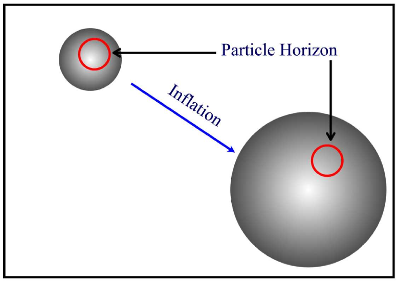
Figure 3: This figure illustrates the expansion from the point of view of an observer located in an embedded dimension. In this way, the observer can ‘look down’ and see the expansion take place. The spacetime is seen to expand from under the particle horizon.

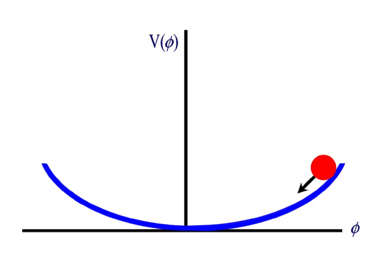
Figure 6: Evolution of the Inflaton Field

In this model of inflation the inflaton finds itself trapped in a false minimum. It is freed from this minimum when tunneling is allowed to occur resulting in a first order phase transition in the early universe.

Table 1: Summary of Friedman Models

Density $\rho$	Pressure $p$	$\alpha$	Epoch
$\rho_{R}$	$\frac{\rho}{3}$	$\frac{1}{3}$	Radiation Dominated
$\rho_{M}$	0	0	Matter Dominated (Non-relativistic Dust)
$\rho_{\Lambda}$	$-\rho$	-1	Vacuum Domination

Table 2: Cosmological Models of a Matter Dominated Universe

Geometry	$\Omega$	$q_{0}$	Fate of Universe	Name
Flat	$=1$	$\frac{1}{2}$	Open Universe	Einstein-DeSitter Model
Hyperbolic	$<1$	$<\frac{1}{2}$	Open Universe	Open Model
Spherical	$>1$	$>\frac{1}{2}$	Closed Universe	Closed Model

References

- (1) R. A. Alpher and R. C. Herman, Phys. Rev. 75, 1089 (1949).
- (2) G. Gamow, The Creation of the Universe (Viking Press, New York, 1952).
- (3) R. H. Dicke, P. J. E. Peebles, P. G. Roll, and D. T. Wilkinson, Ap. J. 142, 414 (1965).
- (4) R. B. Partridge, 3K: The Cosmic Microwave Background Radiation (Cambridge University Press, 1995).
- (5) M. S. Turner and E. W. Kolb, The Early Universe (Addison-Wesley Publishing Company, 1990).
- (6) A. Melchiorri et al. (1999), eprint astro-ph/9911445.
- (7) A. E. Lange et al. (2000), eprint astro-ph/0005004.
- (8) J. R. Hawley and K. A. Holcomb, Foundations of Modern Cosmology (Oxford University Press, 1998).
- (9) S. Hawking and G. Ellis, The Large Scale Structure of Space-Time (Cambridge University Press, 1975).
- (10) J. Narlikar, Introduction to Cosmology (Cambridge University Press, 1995).
- (11) L. Bergström and A. Goobar, Cosmology and Particle Astrophysics (Praxis Publishing Ltd., England, 1999).
- (12) A. Filippenko, Understanding the Universe: An Introduction to Astronomy, The Teaching Company, Video Series (1999).
- (13) T. Richtler and G. Drenkhahn, Cosmology and Astrophysics: A collection of critical thoughts. (not yet published) Eprint astro-ph/9909117 (Springer, 1999).
- (14) C. M. Will, Theory and Experiment in Gravitation Physics (Cambridge University Press, 1981).
- (15) P. Collins, A. Martin, and E. Squires, Particle Physics and Cosmology (John Wiley and Sons, 1989).
- (16) R. J. Finkelstein, Thermodynamics and Statistical Physics: A Short Introduction (W.H. Freeman and Company, 1969).
- (17) A. Dekel and J. P. Ostriker, Formation of Structure in the Universe (Cambridge University Press, 1999).
- (18) N. J. Cornish and J. R. Weeks, Notices of the American Mathematical Society 45(11), 1463 (1998).
- (19) J.-P. Luminet, G. D. Starkman, and J. R. Weeks, Scientific American pp. 90–97 (1999).
- (20) D. Kirkman, D. Tytler, S. Burles, D. Lubin, and J. M. O’meara (1999), eprint astro-ph/9907128.
- (21) M. Arnould, S. Goriely, and A. Jorissen (1999), eprint astro-ph/9904407.
- (22) C. J. Hogan (1997), eprint astro-ph/9712031.
- (23) F. Hamann and G. Ferland (1999), eprint astro-ph/9904223.
- (24) J. A. Peacock, Cosmological Physics (Cambridge University Press, 1999).
- (25) J. Peebles, Principles of Physical Cosmology (Princeton University Press, 1993).
- (26) B. Greene, The Elegant Universe (WW Norton and Company, 1999).
- (27) M. Gaperini, Superstring Cosmology, http://www.to.infn.it/gasperini (1999).
- (28) COBE Homepage, http://space.gsfc.nasa.gov/astro/cobe/ (1992).
- (29) R. A. Serway, C. J. Moses, and C. A. Moyer, Modern Physics (Saunders College Publishing, 1997).
- (30) P. A. Tipler and R. A. Llewellyn, Modern Physics (W.H. Freeman and Company, 1999).
- (31) C. E. Rolfs and W. S. Rodney, Cauldrons in the Cosmos: Nuclear Astrophysics (University of Chicago Press, 1988).
- (32) A. R. Liddle (1999), eprint astro-ph/9901124.
- (33) Y. Fujii (2000), eprint gr-qc/0001051.
- (34) F. Rosati (1999), eprint hep-ph/9908518.
- (35) P. Brax and J. Martin (1999), eprint astro-ph/9912046.
- (36) A. H. Guth, Phys. Rev. D23, 347 (1981).
- (37) A. H. Guth and P. J. Steinhardt, Scientific American (1984).
- (38) S. Weinberg, Gravitation and Cosmology (John Wiley and Sons, 1972).
- (39) D. J. Griffiths, Introduction to Elementary Particles (John Wiley and Sons, Inc., 1989).
- (40) P. Strange, Relativistic Quantum Mechanics (Cambridge University Press, 1998).
- (41) M. Kaku, Quantum Field Theory: A Modern Introduction (Oxford University Press, 1993).
- (42) A. Salam, Elementary Particle Theory (Almquist and Forlag, 1968).
- (43) S. Weinberg, Phys. Rev. Lett. 19, 1264 (1967).
- (44) L. H. Ryder, Quantum Field Theory (Cambridge University Press, 1996).
- (45) B. Zeldovich and M. Khlopov, Phys. Lett. 79B, 239 (1978).
- (46) J. Preskill, Phys. Rev. Lett. 43, 1365 (1979).
- (47) S. Blau and A. Guth, 300 Years of Gravitation (Cambridge University Press, 1987).
- (48) A. H. Guth (2000), eprint astro-ph/0002188.
- (49) A. H. Guth (2000), eprint astro-ph/0002156.
- (50) A. Linde, Zh. Eksp. Teor. Fiz. 38, 149 (1983).
- (51) A. R. Liddle and D. H. Lyth, Phys. Lett. B 291, 391 (1992).
- (52) A. Ghosh, R. Madden, and G. Veneziano (1999), eprint hep-th/9908024.
- (53) H. Maris and S. Balibar, Physics Today pp. 29–34 (2000).
- (54) C. Kittel and H. Kroemer, Thermal Physics (W.H. Freeman and Company, 1980).
- (55) A. D. Linde, Phys. Lett. B 108, 389 (1982).
- (56) A. Albrecht and P. J. Steinhardt, Phys. Rev. Lett. 48, 1220 (1982).
- (57) A. Linde, Phys. Lett. 129B, 177 (1983).
- (58) A. Linde, Phys. Lett. B175, 395 (1986).
- (59) A. Linde, Scientific American 271(5), 48 (1994).
- (60) A. Linde, Phys.Rev. D 59 (1999), eprint astro-ph/9807493.
- (61) S. Hawking and N. Turok, Phys. Lett. B B432, 271 (1998), eprint astro-ph/9807493.
- (62) Y. B. Zeldovich, Astr. Astrophys. 5 (1970).
- (63) G. S. et. al., Astrophys. Journ. 396 (1992).
- (64) S. Carroll, submitted to: Living Reviews in Relativity (2000).
- (65) W. Hu, U. Seljak, M. White, and M. Zaldarriaga (1998), eprint asto-ph/9709066v2.
- (66) W. Hu (2000), eprint asto-ph/0002520.
- (67) W. Hu, The Universe at High-z, Large Scale Structure and the CMB .
- (68) R. Brandenberger, H. Feldman, and V. Mukhanov, Phys. Reports 215 (1992).
- (69) J. Lidsey and et. al., Reviews of Modern Physics 69 (1997).
- (70) D. H. Lyth and L. Covi (2000), eprint astro-ph/0002397.
- (71) D. H. Lyth (1996).
- (72) W. Hu, Web-Page On CMB, http://www.sns.ias.edu/whu/cmbex.html (2000).
- (73) R. Brandenberger and J. Magueijo (2000).
- (74) M. Kamionkowski (1998), eprint astro-ph/9808004.
- (75) M. Turner and L. Widrow, Phys. Rev. D 30, 2743 (1988).
- (76) A. R. Liddle (1999), eprint astro-ph/9910110.
- (77) J. Jackson, Classical Electrodynamics (John Wiley and Sons, Inc., 1999).
- (78) M. Kamionkowski, A. Kosowsky, and A. Stebins, Phys. Rev. D 55, 7368 (1997).