First Estimations of Cosmological Parameters from Boomerang

Abstract

The anisotropy of the cosmic microwave background radiation contains information about the contents and history of the universe. We report new limits on cosmological parameters derived from the angular power spectrum measured in the first Antarctic flight of the Boomerang experiment. Within the framework of inflation-motivated adiabatic cold dark matter models, and using only weakly restrictive prior probabilites on the age of the universe and the Hubble expansion parameter $h$, we find that the curvature is consistent with flat and that the primordial fluctuation spectrum is consistent with scale invariant, in agreement with the basic inflation paradigm. We find that the data prefer a baryon density $\Omega_{b}h^{2}$ above, though similar to, the estimates from light element abundances and big bang nucleosynthesis. When combined with large scale structure observations, the Boomerang data provide clear detections of both dark matter and dark energy contributions to the total energy density $\Omega_{\rm{tot}}$, independent of data from high redshift supernovae.

The angular power spectrum ${\cal C}_{\ell}$ of temperature anisotropy in the cosmic microwave background (CMB) is a powerful probe of the content and nature of the universe. The DMR instrument on the COBE satellite measured ${\cal C}_{\ell}$ for multipoles $\ell\mathrel{\hbox to0.0pt{\lower 3.0pt\hbox{$\mathchar 536\relax$}\hss}\raise 2.0pt\hbox{$\mathchar 316\relax$}}20$, corresponding to angular scales $\mathrel{\hbox to0.0pt{\lower 3.0pt\hbox{$\mathchar 536\relax$}\hss}\raise 2.0pt\hbox{$\mathchar 318\relax$}}7^{\circ}$Bennett96 . Significant experimental effort by many groups focusing on smaller angular scales, when combined BJK98 ; toco98 ; mauskopf99 , led to the ${\cal C}_{\ell}$ estimates in the $\ell$ bands marked with x’s in Figure 1, which indicate a peak at $\ell\sim 200$knox2000 . It has long been recognized that if ${\cal C}_{\ell}$ can be determined with high precision over these angular scales, parameters such as the total energy density and baryon content of the universe, and the shape of the primordial power spectrum of density fluctuations, can be accurately measured BET97 . The most recently published Boomerang angular power spectrum shown in Figure 1 represents a qualitative step towards such high precision debernardis00 (hereafter, B98).

The data define a strong peak at $\ell\sim 200$. The steep drop in power from $\ell\sim 200$ to $\ell\sim 400$ is consistent with the structure expected from acoustic oscillations in adiabatic cold dark matter (CDM) models of the universe, but is not consistent with the locations and widths of peaks expected in the simplest cosmic string, global topological defect, and isocurvature perturbation models defects . The data at higher $\ell$ show strong detections which limit the height of a second peak, but are consistent with the height expected in many CDM models.

In this paper, we concentrate on determining a set of 7 cosmological parameters that characterize a very broad class of CDM models by statistically confronting the theoretical ${\cal C}_{\ell}$’s with the B98 and DMR data. Sample CDM models that fit the data are shown in Figure 1. These are best-fit theoretical models using successively more restrictive “prior probabilities” on the parameters. A major theme of this paper is to illustrate explicitly how inferences that are drawn from the CMB data depend on the priors that are assumed. Some of these priors are quite weakly restrictive and are generally agreed upon by most cosmologists, for example that the Universe is older than 10 Gyr and that the Hubble constant $H_{0}=100\,h\mbox{\, km s}^{-1}\mbox{Mpc}^{-1}$ lies between 45 and 90. More strongly restrictive priors rely on specific measurements, e.g., the HST key project determination of $H_{0}$ to 10% accuracy hstkeyproj and the determination of the cosmological baryon density, $\omega_{b}\equiv\Omega_{b}h^{2}$, to 10% BBN .

In debernardis00 , we applied a “medium” set of priors to the B98 power spectrum to constrain a 6 cosmological parameter model and found a 95% confidence limit for $\Omega_{\rm{tot}}$ of $0.88<\Omega_{\rm{tot}}<1.12$. Row P0 of Table 1 shows the result for our full 7 parameter set with a similar medium prior (here taken to be $h=0.65\pm 0.1$, $\omega_{b}=0.019\pm 0.006$, with Gaussian errors for both). As we progress through the Table, we show the effect of either weakening or strengthening the prior from this starting point.

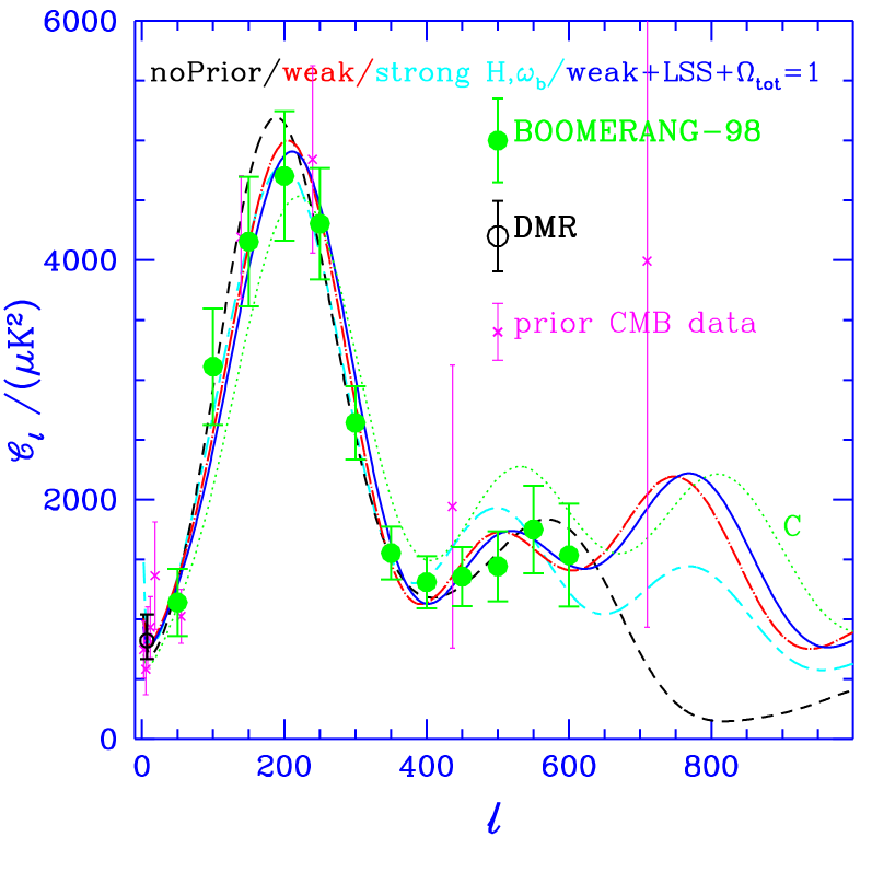
Figure 1: CMB angular power spectra, ${\cal C}_{\ell}\equiv\ell(\ell+1)\langle|T_{\ell m}|^{2}\rangle/(2\pi)$, where the $T_{\ell m}$ are the multipole moments of the CMB temperature. The closed (green) circles show the B98 data. The magenta crosses are a radical compression of all the data prior to B98 into optimal bandpowers BJK98 ; toco98 ; mauskopf99 , showing the qualitative improvement provided by B98 except in the $\ell\mathrel{\hbox to0.0pt{\lower 3.0pt\hbox{$\mathchar 536\relax$}\hss}\raise 2.0pt\hbox{$\mathchar 316\relax$}}20$ DMR regime, where the COBE data are represented as a single bandpower (open black circle). (Note that the B98 and prior CMB points at $\ell=150$ lie on top of each other.) The smooth curves depict power spectra for several maximum likelihood models with different priors chosen from Table 1, with ($\Omega_{\rm{tot}},\omega_{b},\omega_{c},\Omega_{\Lambda},n_{s},\tau_{c}$) as follows: P1, short dashed line,(1.3,0.10,0.80,0.6,0.80,0.025); P4, dot-dashed line,(1.15,0.03,0.17,0.4,0.925,0); P8, short-long dashed line,(1.05,0.02,0.06,0.90,0.825,0); P11, solid line,(1.0,0.03,0.17,0.70,0.95,0.025). These curves are all reasonable fits to the B98+COBE data. For comparison, we plot a $H_{0}=68$, $\Omega_{\Lambda}=0.7$ “concordance model” which does not fit (dotted line labelled C), with parameters (1.0,0.02,0.12,0.70,1.0,0).

Two of our parameters are fundamental for describing the physics of the radiative transport of the CMB through the epoch at $z\sim 1100$, when the photons decoupled from the baryons. These are $\omega_{b}$ and the CDM density $\omega_{c}\equiv\Omega_{c}h^{2}$. The acoustic patterns at decoupling are related to the sound-crossing distance at that time, $r_{s}$, which is sensitive to these parameters. We fix the density of photons and neutrinos mnu , which are other important constituents at this epoch. The observed B98 patterns are also sensitive to the “angular diameter distance” to photon decoupling, mapping the $z\sim 1100$ spatial structure to the angular structure, and, through its dependence on geometry, to $\Omega_{\rm{tot}}$, the total energy in units of the critical density. When $\Omega_{\rm{tot}}<1$ (open models), $r_{s}$ is mapped to a small angular scale; when $\Omega_{\rm{tot}}>1$ (closed models), $r_{s}$ is mapped to a large angular scale.

This mapping also depends upon the density associated with a cosmological constant, $\Omega_{\Lambda}$, and $\Omega_{m}\equiv(\omega_{c}+\omega_{b})/h^{2}$, as well as on $\Omega_{k}\equiv 1-\Omega_{\rm{tot}}$, the density associated with curvature. Combinations of $\Omega_{k}/\Omega_{m}$ and $\Omega_{\Lambda}/\Omega_{m}$ which give the same ratio of angular diameter distance to sound horizon will give nearly identical CMB patterns, resulting in a near degeneracy that is broken only at large angular scales where photon transport through time-varying gravitational potentials plays a role. One implication of this is that $\Omega_{\Lambda}$ cannot be well determined by our data alone, in spite of the high precision of B98. We have paid special attention to such near-degeneracies EB98 throughout our analysis.

The universe reionized sometime between photon decoupling and $z\sim 5$. This suppresses ${\cal C}_{\ell}$ at small scales by a factor $e^{-2\tau_{c}}$, where $\tau_{c}$, our fifth parameter, is the optical depth to Thompson scattering from the epoch at which the universe reionized to the present.

Our last two parameters characterize the nature of the fluctuations arising in the very early universe, through a power law “tilt” $n_{s}$ and an overall amplitude factor for the primordial perturbations. The simplest inflation models have a nearly scale invariant spectrum characterized by $n_{s}\approx 1$. Of course, many more variables, and even functions, may be needed to specify the primordial fluctuations, in particular those describing the possible contribution of gravity waves, whose role we have also tested gw . For our overall amplitude parameter, we use $\ln{\cal C}_{10}$ where ${\cal C}_{10}$ is the CMB power in the theoretical spectrum at $\ell=10$. If we wish to relate the CMB data to large scale structure (LSS) observations of the Universe, we use $\ln\sigma_{8}^{2}$ as the amplitude parameter, where $\sigma_{8}^{2}$ is the model power in the density fluctuations on the scale of clusters of galaxies ($8h^{-1}\mbox{Mpc}$).

Our adopted parameter space is therefore $\{\omega_{b},\omega_{c},\Omega_{\rm{tot}},\Omega_{\Lambda},n_{s},\tau_{c},\ln{\cal C}_{10}\}$. The amplitude ${\cal C}_{10}$ is a continuous variable, and the rest are discretized for the purpose of constructing the model database we use to compare data and theory. The number of values and coverage are: 15, over $0.1\mathrel{\hbox to0.0pt{\lower 3.0pt\hbox{$-$}\hss}\raise 2.0pt\hbox{$\mathchar 316\relax$}}\Omega_{\rm{tot}}\mathrel{\hbox to0.0pt{\lower 3.0pt\hbox{$-$}\hss}\raise 2.0pt\hbox{$\mathchar 316\relax$}}1.5$; 14, over $0.0031\mathrel{\hbox to0.0pt{\lower 3.0pt\hbox{$-$}\hss}\raise 2.0pt\hbox{$\mathchar 316\relax$}}\omega_{b}\mathrel{\hbox to0.0pt{\lower 3.0pt\hbox{$-$}\hss}\raise 2.0pt\hbox{$\mathchar 316\relax$}}0.2$; 10, over $0.03\mathrel{\hbox to0.0pt{\lower 3.0pt\hbox{$-$}\hss}\raise 2.0pt\hbox{$\mathchar 316\relax$}}\omega_{c}\mathrel{\hbox to0.0pt{\lower 3.0pt\hbox{$-$}\hss}\raise 2.0pt\hbox{$\mathchar 316\relax$}}0.8$; 11, over $0\mathrel{\hbox to0.0pt{\lower 3.0pt\hbox{$-$}\hss}\raise 2.0pt\hbox{$\mathchar 316\relax$}}\Omega_{\Lambda}\mathrel{\hbox to0.0pt{\lower 3.0pt\hbox{$-$}\hss}\raise 2.0pt\hbox{$\mathchar 316\relax$}}1.1$; 9, over $0\mathrel{\hbox to0.0pt{\lower 3.0pt\hbox{$-$}\hss}\raise 2.0pt\hbox{$\mathchar 316\relax$}}\tau_{c}\mathrel{\hbox to0.0pt{\lower 3.0pt\hbox{$-$}\hss}\raise 2.0pt\hbox{$\mathchar 316\relax$}}0.5$; 31, over $0.5\mathrel{\hbox to0.0pt{\lower 3.0pt\hbox{$-$}\hss}\raise 2.0pt\hbox{$\mathchar 316\relax$}}n_{s}\mathrel{\hbox to0.0pt{\lower 3.0pt\hbox{$-$}\hss}\raise 2.0pt\hbox{$\mathchar 316\relax$}}1.5$. The spacings in each dimension are uneven, designed to concentrate coverage in the regions preferred by the data and yet still map the outlying regionsdatabase . Fast CMB transport programs CMBFASTCAMB were used to construct our ${\cal C}_{\ell}$ databases. Use was made of the angular-diameter distance degeneracy and $\ell$-space compression to reduce the size and computational requirements needed to construct such a database.

Parameter estimation is an integral part of the B98 analysis pipeline, which makes statistically well-defined maps and corresponding noise matrices from the time-ordered data, from which we compute a set of maximum likelihood bandpowers, ${\cal C}_{B}$. The likelihood curvature matrix ${\cal F}_{BB^{\prime}}$ is calculated to provide error estimates including correlations between bandpowers. The curvature matrix ${\cal F}_{BB^{\prime}}$ and the curvature matrix evaluated at zero signal, ${\cal F}_{BB^{\prime}}^{0}$, are used in the offset-lognormal approximation BJK98 to compute likelihood functions $L(x,\vec{y})=P(\vec{\cal C}_{B}|x,\vec{y})$ for each combination of parameters $x$ and $\vec{y}$ in our database. Here $x$ is the value of the parameter we are limiting, $\vec{y}$ specifies the values of the other parameters.

We multiply the likelihood by our chosen priors, and marginalize over the values of the other parameters $\vec{y}$, including the systematic uncertainties in the beamwidth and calibration of the measurement beam . This yields the marginalized likelihood distribution

$$\mathcal{L}(x)\equiv P(x|\vec{\cal C}_{B})=\int P_{prior}(x,\vec{y})L(x,\vec{y})d\vec{y}.$$ (1)

For clear detections, central values and $1\sigma$ limits for the explicit database parameters mentioned above are found from the 16%, 50% and 84% integrals of $\mathcal{L}(x)$. When no clear detection exists, these errors can be misleading, so for these cases we shift to likelihood falloffs by $e^{-1/2}$ from the maximum, or variances about the mean of the distribution $\mathcal{L}(x)$. The mean and variance are used to set the limits on other “auxiliary” parameters such as $h$ and $\Omega_{m}$, which may be nonlinear combinations of the database variables. For good detections the three estimation methods give very good agreement, and yield 2$\sigma$ errors that are roughly twice the 1$\sigma$ ones generally reported in this paper.

We have used this method to estimate parameters, using the B98 power spectrum of Figure 1 with the COBE bandpowers determined by BJK98 and a variety of priors. The results are summarized in Table 1; likelihood functions for selected parameters and priors are shown in Figure 2.

In the presence of degenerate and ill-constrained combinations of parameters, as with CMB data, the edges of the data-base form implicit priors. We have constructed our database such that these effective priors are extremely broad. This allows us to probe the dependence of our results on individually imposed priors. The choice of measure on the space is itself a prior; we have used a linear measure in each of our variables measure . Sufficiently restrictive priors can break parameter degeneracies and result in more stringent limits on the cosmological parameters. Artificially restrictive databases or priors can lead to misleading results; thus, priors should be both well motivated and tested for stability. We therefore regard it as essential that the role of “hidden priors” in any choice for ${\cal C}_{\ell}$ database construction be clearly articulated.

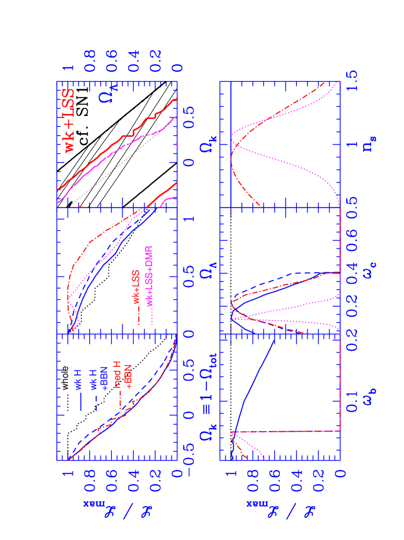
Figure 3: Likelihood functions similar to those in Figure 2, but computed without using the B98 data. These curves show the effect of the database constraints and applied priors alone. The identification of the curves is the same as in Figure 2, with the addition of the dotted magenta curve in panels 2-6, which shows the likelihood given weak priors and the COBE DMR data. In panel 3, only the 1$\sigma$ (red) contour is shown for the prior only and prior+DMR cases, while 1, 2 and 3$\sigma$ (light black) contours are shown for SN1a. The curves for P2 (solid blue) and P4 (dashed blue) are slightly separated in this figure, in contrast to Figure 2, where they overlapped. Of particular interest here are the slope induced across $\Omega_{k}$, the slight localization of $\Omega_{c}h^{2}$ with the weak priors, and the significant localization of $\Omega_{c}h^{2}$ and $n_{s}$ with just weak+DMR+LSS (dotted magenta).

To illustrate the effects of the database structure and applied priors, we have plotted likelihood functions found using only the database and priors (and no B98 data) in Figure 3. These should be compared with those plotted in Figure 2 which include the B98 constraints, as discussed below. We now turn to the results found by applying different priors, in the general order of weakest to strongest applied priors.

Our “entire database” analysis prefers closed models with very high $\omega_{b}$, as shown in line P1 of Table 1 and in Figure 2. The low sound speed of these models couples with the closed geometry to fit the peak near $\ell\sim 200$. These models require very high values of $h$ and $\omega_{b}$, and have extremely low ages, so we have mapped out this region using a coarse grid. The dual-peaked projected likelihood functions shown are reflections of the the complexity of the full 9-dimensional likelihood hypersurface. We note that parameter combinations that appear to have a low probability based on the projected one-dimensional limits can fit the data quite well, e.g., the $\Omega_{\rm{tot}}=1$ best-fit model of Figure 1.

Applying weakly restrictive priors (lines P2-P4 in Table 1) moves the result away from the low sound speed models, to a regime which is stable upon application of more restrictive priors, as shown in panels 1 (top left) and 4 (bottom left) of Figure 2. Given their gross conflict with many other cosmological tests we do not advocate the “entire database” models as representative of the actual universe, and we proceed with prior-limited analyses below.

The analysis with weakly restrictive priors (P2-P4) finds that the curvature is consistent with flat, while favoring slightly closed models. The migration toward $\Omega_{k}=0$ as more restrictive priors are applied, as shown in Table 1 and in panel 1 (top left) of Figure 2, suggests caution in drawing any conclusion from the magnitude of the likelihood drop at $\Omega_{k}=0$. In fact, as is evident from Figure 1, there are models with $\Omega_{k}=0$ that fit the data quite well. The likelihood curve simply indicates that there are more models with $\Omega_{k}<0$ than with $\Omega_{k}>0$ that fit the data well.

We have taken special care to study the effect on the likelihood distributions of choosing a different parameterization of our database. For example, we have investigated the likelihoods that result from a finely gridded database that uses $\Omega_{c}$, $\Omega_{b}$, and $h$ in place of $\Omega_{k}$, $\omega_{b}$, and $\omega_{c}$ to determine $\Omega_{k}$. This second method, restricted to $\tau_{c}=0$ models, uses these different variable choices, gridding, and a completely different procedure and code which uses maximization of the likelihood over other variables rather than marginalization. To compare with this second method, we have taken the database used for the table and mimicked the effective priors due to the parameter limits of the second database. The results found using these two parameterizations and codes agree quite well - in all cases the likelihood curves shift by at most a small fraction of their width. For example, for the applied priors of P2 the 95% confidence limits on $\Omega_{{\rm tot}}$ shift from $0.99<\Omega_{{\rm tot}}<1.24$ for the method used in the table to $0.94<\Omega_{{\rm tot}}<1.27$ for the $\Omega_{c}$, $\Omega_{b}$, and $h$ method. Due to the very steep slope of the likelihood near $\Omega_{k}=0$, however, even this small shift changes $L(\Omega_{k}=0)/L_{max}$ from 0.2 to 0.8. We also find $L(\Omega_{k}=0)/L_{max}\approx 0.8$ if we use maximization, rather than marginalization, in the code used for the table. Additionally, we note that a downward shift of about 5% in $\Omega_{{\rm tot}}$ occurs if the 10 Gyr age constraint is removed from P2. These points, plus the obvious compatibility of the data with the best-fit $\Omega_{tot}=1$ curve in Fig. 1, reinforces our conclusion that there is no significant evidence in the B98 data for non-zero curvature. The only valid conclusion to draw from the data that we analyze in this paper is that the geometry of the universe is very close to flat.

The baryon density $\omega_{b}$ is also well constrained. While our results are higher ($\sim 3\sigma$) than the $\omega_{b}$ estimates from light element abundances BBN , it is most remarkable that our entirely independent method yields a result that is so close to the BBN value. The scalar spectral index $n_{s}$ is very stable once weak priors are applied, and is near the value expected from inflation. This weak prior analysis does not yield a significant detection of $\Omega_{\Lambda}$; the $\Omega_{c}h^{2}$ results in Table 1 are suggestive of a detection, but are at least in part driven by the weak priors acting on limits of the database hiddenpriors1 ; hiddenpriors2 as shown in Figure 3. The values of $\tau_{c}$ are in the range of expectation of the models, but there is no clear detection.

Note that the the weak priors adopt the conservative restriction that the age of the universe exceeds 10 Gyr. Without this, the weak $h$ prior still allows a contribution, albeit reduced, from the high $\omega_{b}$, low sound speed, low age solution. With the age restriction, this solution is eliminated, and the weak BBN prior ($\omega_{b}\mathrel{\hbox to0.0pt{\lower 3.0pt\hbox{$-$}\hss}\raise 2.0pt\hbox{$\mathchar 316\relax$}}0.5$) does not significantly change the constraint: thus, the “weak $h$+BBN+age” (P4) and “weak $h$+age” (P2) rows are essentially identical.

In row P4a, we add a “CMB prior”, which is a full likelihood analysis of all prior CMB experiments combined with B98 and DMR, including appropriate filter functions, calibration uncertainties, correlations, and noise estimates for use in the offset-lognormal approximation BJK98 . As would be expected given the errors we compute on the compressed bandpowers of these experiments in Figure 1 cf. those for B98, this CMB prior only slightly modifies the B98-derived parameters, with $n_{s}$ the most notable migration. None the less, as much previous analysis of the prior heterogeneous CMB datasets has shown otherparamest , reasonably strong cosmological conclusions could already be drawn on $n_{s}$ and $\Omega_{\rm{tot}}$. Row P4b shows results excluding B98, for the weak prior case, through our machinery. Though $n_{s}$ and $\Omega_{k}$ have detections consistent with the B98 results, no conclusions can be drawn on $\omega_{b}$ (though the “whole database” analysis does pick up the high $\omega_{b}$, $\Omega_{\rm{tot}}$ region). We note that if $\tau_{c}\approx 0$ is enforced, most variables remain unmoved, but $n_{s}$, which is well-correlated with $\tau_{c}$, moves closer to unity: for P4, P4a, P4b, we would have $n_{s}=0.97,1.03,1.02$, respectively, and for P5, P5a, P5b, we would have $n_{s}=0.93,0.98,0.98$. A prior probability of $\tau_{c}$ based on ideas of early star formation would help to decrease the $n_{s}$ degree of freedom.

The $\Omega_{\rm{tot}}$, $\omega_{b}$, and $n_{s}$ results are stable to the addition of a prior which imposes two constraints derived from LSS observations BJ98 . The first is an estimate of $\sigma_{8}^{2}$ that requires the theory in question to reproduce the local abundance of clusters of galaxies. The second is an estimate of a shape parameter for the density power spectrum derived from observations of galaxy clustering LSS . Adding LSS to the weak $h$ and BBN priors (P5, and panels 2 (top center) and 3 (top right) of Figure 2) breaks a degeneracy, yielding a detection of $\Omega_{\Lambda}$ that is consistent with “cosmic concordance” models. This also occurs when LSS is added to only the prior CMB data (P5b and BJ98 ). The LSS prior also strengthens the statistical significance of the determination of $\Omega_{c}h^{2}$. Panel 3 (top right) of Figure 2 shows likelihood contours in the $\Omega_{k}\equiv 1-\Omega_{\rm{tot}}$ vs. $\Omega_{\Lambda}$ plane. Here we have plotted the LSS prior (P5), which strongly localizes the contours contourerrors away from the $\Omega_{\Lambda}=0$ axis, toward a region that is highly consistent with the SN1a results SN1a . Indeed, treating the SN1a likelihood as a prior does not change the results very much, as indicated by row P12 and P13 of the Table, to be compared with rows P5 and P11, respectively.

The use of a strong $h$ prior alone yields results very similar to those for the weak $h$ case. The strong BBN prior, however, shifts many of the results from the weak BBN case. Our data indicate a higher $\Omega_{b}h^{2}$ than BBN, and constraining it with the BBN prior shifts the values of several parameters, including $\Omega_{c}h^{2}$, $\Omega_{\Lambda}$, $n_{s}$, and $\Omega_{m}$. Additional “strong prior” results (P8-P11) are shown in Table 1, as an exercise in the power of combining other constraints with CMB data of this quality.

A number of the cosmological parameters are highly correlated, reflecting weak degeneracies in the broad but restricted $\ell$-space range that the B98+DMR data covers EB98 . Some of these degeneracies can be broken with data at higher $\ell$, as is visually evident in the radically different behavior of the models of Figure 1 beyond $\ell\sim 600$. To understand the degeneracies within the context of this data, we have explored the structure of the parameter covariance matrix $\langle\Delta y_{i}\Delta y_{j}\rangle$, both for the database parameters and the ones derived from them. They add motivation for the specific parameter choices we have made rcorr . Parameter eigenmodes BET97 ; EB98 of the covariance matrix, found by rotating into principal components, explicitly show the combinations of physical database variables that give orthogonal error bars. A by-product is a rank-ordered set of eigenvalues, which show that for the current B98 data, 3 combinations of the 7 parameters are determined to better than $10\%$ parameigen .

We conclude that the B98 data are consistent with the predictions of the basic inflationary paradigm: that the curvature of the universe is near zero ($\Omega_{k}=0$) and that the primordial power spectrum is nearly scale-invariant ($n_{s}=1$). The slight preference that the current data show for closed, rather than open, models is not, we believe, a statistically significant indication of non-zero curvature. A more conclusive statement awaits further analysis of B98 data, which will increase the precision of the measured power spectrum, and/or the results from other experiments.

We measure a strong detection of the baryon density $\Omega_{b}h^{2}$, a first for determinations of this parameter from CMB data. The value that we measure is robust to the choice of prior, and is both remarkably close to and significantly higher than that given by the observed light element abundances combined with BBN theory. Assuming that $\Omega_{{\rm tot}}=1$, we find $\Omega_{b}h^{2}=0.031\pm 0.004$.

Finally, we find that combining the B98 data with our relatively weak prior representing LSS observations and with our other weak priors on the Hubble constant and the age of the universe yields a clear detection of both non-baryonic matter ($\Omega_{c}h^{2}=0.014^{+0.003}_{-0.002}$) and dark energy ($\Omega_{\Lambda}=0.66^{+0.07}_{-0.09}$) contributions to the total energy density in the universe. The amount of dark energy that we measure is robust to the inclusion of a prior on $\Omega_{{\rm tot}}$ (shifting to $\Omega_{\Lambda}=0.67^{+0.04}_{-0.06}$ for $\Omega_{{\rm tot}}=1$), and to the inclusion of the prior likelihood given by observations of high-redshift SN1a (shifting to $\Omega_{\Lambda}=0.69^{+0.02}_{-0.03}$ when both the $\Omega_{{\rm tot}}=1$ and the SN1a priors are included). The perfect concordance between the completely independent detections of $\Omega_{\Lambda}$ from the CMB+LSS data and from the SN1a data is powerful support for the notion that the universe is currently dominated by precisely the amount of dark energy necessary to provide zero curvature.

The analysis presented here and in debernardis00 makes use of only a small fraction of the data obtained during the first Antarctic flight of Boomerang. Work now in progress will increase the precision of the power spectrum from $\ell=50$ to 600, and extend the measurements to smaller angular scales, allowing yet more precise determinations of several of the cosmological parameters.

Table 1: Results of parameter extraction using successively more restrictive priors. The confidence intervals are 1$\sigma$, evaluated using methods described in the text. The 2$\sigma$ errors are approximately double the 1$\sigma$ values quoted in most cases; upper limits are quoted at 2$\sigma$. The quoted values are reported after marginalizing over all other parameters. Note that these combinations are not, and should not be, the parameters of the “maximum likelihood” best-fit models of Figure 1. The weak $h$ and BBN ($\Omega_{b}h^{2}$) priors are tophat functions (uniform priors) and both include an additional age $>10$ Gyr prior. The strong priors are Gaussians with the stated 1$\sigma$ error, and also have weak constraints imposed on the other variables. P0 is the medium $h$ + BBN prior used in debernardis00 and described in the text. The LSS priors are combinations of Gaussians and tophats LSS . The SN1 prior (P12, P13) includes LSS as well the SN1a likelihood shown in panel 3 of Fig. 2. P4a and P5a show the small effect of including prior CMB data in our B98+DMR analysis; these should be contrasted with P4b and P5b, the case of prior CMB data alone. Columns 1-5 ($\Omega_{\rm{tot}}$ to $\Omega_{\Lambda}$) are predominantly driven by the CMB data, except for $\Omega_{b}h^{2}$ and $\Omega_{b}$ when the strong BBN prior (P7-P9) is applied. Most of the values in columns 6-10 ($\tau_{c}$ to Age) are influenced by the structure of the parameter space and should not be interpreted as CMB-driven constraints; exceptions are the $\Omega_{c}h^{2}$ and $\Omega_{\Lambda}$ results when the LSS prior is applied. An equivalent table that includes an inflation-inspired gravity wave induced contribution to the anisotropy gw yields remarkably similar parameters and errors.

Priors	$\Omega_{\rm{tot}}$	$\Omega_{b}h^{2}$	$n_{s}$	$\Omega_{b}$	$\Omega_{\Lambda}$	$\tau_{c}$	$\Omega_{c}h^{2}$	$\Omega_{m}$	$h$	Age
P0: Medium $h$+BBN	$1.07^{0.06}_{0.06}$	$0.030^{0.004}_{0.004}$	$1.00^{0.08}_{0.08}$	$0.08^{0.02}_{0.02}$	$0.37^{0.23}_{0.23}$	$0.12^{0.16}_{0.09}$	$0.25^{0.10}_{0.09}$	$0.72^{0.23}_{0.23}$	$0.63^{0.06}_{0.06}$	$11.9^{1.6}_{1.6}$
P1: Whole Database	$1.31^{...}_{0.16}$	$0.100^{0.031}_{0.043}$	$0.88^{0.12}_{0.09}$	$0.10^{0.05}_{0.05}$	$0.53^{0.22}_{0.27}$	$0.22^{0.19}_{0.16}$	…	$0.81^{0.34}_{0.34}$	$1.08^{0.39}_{0.39}$	$7.8^{2.9}_{2.9}$
P2: Weak $h$ ($0.45<h<0.90$)+age	$1.15^{0.10}_{0.09}$	$0.036^{0.006}_{0.005}$	$1.04^{0.10}_{0.09}$	$0.11^{0.04}_{0.04}$	$<0.83$	$0.21^{0.19}_{0.15}$	$0.24^{0.08}_{0.09}$	$0.84^{0.29}_{0.29}$	$0.58^{0.10}_{0.10}$	$12.7^{2.1}_{2.1}$
P3: Weak BBN ($\Omega_{b}h^{2}\mathrel{\hbox to0.0pt{\lower 3.0pt\hbox{$-$}\hss}\raise 2.0pt\hbox{$\mathchar 316\relax$}}0.05$)+age	$1.16^{0.10}_{0.10}$	$0.035^{0.006}_{0.006}$	$1.03^{0.10}_{0.10}$	$0.16^{0.09}_{0.09}$	$<0.83$	$0.21^{0.19}_{0.15}$	$0.19^{0.10}_{0.09}$	$0.92^{0.33}_{0.33}$	$0.52^{0.14}_{0.14}$	$14.6^{3.9}_{3.9}$
P4: Weak $h$+BBN+age	$1.15^{0.10}_{0.09}$	$0.036^{0.005}_{0.005}$	$1.04^{0.10}_{0.09}$	$0.11^{0.04}_{0.04}$	$<0.83$	$0.21^{0.19}_{0.15}$	$0.24^{0.08}_{0.09}$	$0.84^{0.29}_{0.29}$	$0.58^{0.10}_{0.10}$	$12.7^{2.1}_{2.1}$
P4a: Weak and prior CMB	$1.01^{0.09}_{0.09}$	$0.031^{0.007}_{0.006}$	$1.06^{0.10}_{0.09}$	$0.10^{0.04}_{0.04}$	$<0.79$	$0.24^{0.19}_{0.17}$	$0.18^{0.07}_{0.06}$	$0.64^{0.23}_{0.23}$	$0.59^{0.11}_{0.11}$	$13.4^{1.9}_{1.9}$
P4b NO B98: Weak and prior CMB	$1.03^{0.12}_{0.10}$	$0.024^{0.017}_{0.018}$	$1.14^{0.12}_{0.13}$	$0.08^{0.06}_{0.06}$	$<0.80$	$0.29^{0.16}_{0.19}$	$0.21^{0.09}_{0.08}$	$0.71^{0.28}_{0.28}$	$0.60^{0.11}_{0.11}$	$12.9^{2.0}_{2.0}$
P5: LSS & Weak $h$+BBN+age	$1.12^{0.07}_{0.07}$	$0.034^{0.006}_{0.005}$	$0.99^{0.10}_{0.08}$	$0.10^{0.04}_{0.04}$	$0.66^{0.07}_{0.09}$	$0.19^{0.21}_{0.14}$	$0.14^{0.03}_{0.02}$	$0.48^{0.13}_{0.13}$	$0.60^{0.11}_{0.11}$	$14.5^{1.6}_{1.6}$
P5a: LSS & Weak and prior CMB	$1.02^{0.09}_{0.08}$	$0.030^{0.007}_{0.006}$	$1.05^{0.10}_{0.08}$	$0.09^{0.04}_{0.04}$	$0.47^{0.18}_{0.22}$	$0.22^{0.19}_{0.16}$	$0.16^{0.05}_{0.04}$	$0.57^{0.20}_{0.20}$	$0.60^{0.12}_{0.12}$	$13.8^{1.7}_{1.7}$
P5b NO B98: LSS & Weak and CMB	$1.00^{0.07}_{0.07}$	$0.028^{0.015}_{0.015}$	$1.08^{0.11}_{0.11}$	$0.08^{0.06}_{0.06}$	$0.58^{0.13}_{0.17}$	$0.26^{0.17}_{0.18}$	$0.14^{0.04}_{0.03}$	$0.44^{0.15}_{0.15}$	$0.63^{0.12}_{0.12}$	$13.8^{1.7}_{1.7}$
P6: Strong $h$ ($h=0.71\pm 0.08$)	$1.09^{0.07}_{0.06}$	$0.036^{0.005}_{0.005}$	$1.05^{0.09}_{0.09}$	$0.08^{0.03}_{0.03}$	$<0.82$	$0.20^{0.19}_{0.15}$	$0.26^{0.08}_{0.10}$	$0.71^{0.27}_{0.27}$	$0.66^{0.07}_{0.07}$	$11.6^{1.4}_{1.4}$
P7: Strong BBN ($\Omega_{b}h^{2}$=$0.019\pm 0.002$)	$1.10^{0.05}_{0.05}$	$0.021^{0.003}_{0.002}$	$0.85^{0.08}_{0.07}$	$0.07^{0.02}_{0.02}$	$0.79^{0.08}_{0.30}$	$0.09^{0.12}_{0.07}$	$0.08^{0.07}_{0.03}$	$0.38^{0.21}_{0.21}$	$0.54^{0.10}_{0.10}$	$17.7^{2.9}_{2.9}$
P8: Strong $h$+BBN	$1.04^{0.04}_{0.04}$	$0.021^{0.003}_{0.002}$	$0.87^{0.07}_{0.07}$	$0.05^{0.02}_{0.02}$	$0.75^{0.14}_{0.25}$	$0.08^{0.12}_{0.06}$	$0.09^{0.09}_{0.03}$	$0.28^{0.19}_{0.19}$	$0.68^{0.09}_{0.09}$	$15.2^{2.2}_{2.2}$
P9: LSS & Strong $h$+BBN	$1.04^{0.05}_{0.04}$	$0.022^{0.003}_{0.002}$	$0.92^{0.06}_{0.06}$	$0.05^{0.02}_{0.02}$	$0.66^{0.05}_{0.07}$	$0.08^{0.12}_{0.06}$	$0.14^{0.03}_{0.02}$	$0.39^{0.07}_{0.07}$	$0.64^{0.08}_{0.08}$	$14.0^{1.3}_{1.3}$
P10: $\Omega_{\rm{tot}}=1$ & Weak $h$+age	1	$0.031^{0.004}_{0.004}$	$0.99^{0.07}_{0.07}$	$0.06^{0.02}_{0.02}$	$<0.78$	$0.10^{0.13}_{0.07}$	$0.27^{0.05}_{0.07}$	$0.57^{0.21}_{0.21}$	$0.74^{0.09}_{0.09}$	$10.9^{0.8}_{0.8}$
P11: $\Omega_{\rm{tot}}=1$ & LSS & Weak	1	$0.030^{0.004}_{0.004}$	$0.96^{0.07}_{0.06}$	$0.05^{0.01}_{0.01}$	$0.67^{0.04}_{0.06}$	$0.09^{0.12}_{0.07}$	$0.18^{0.02}_{0.02}$	$0.32^{0.05}_{0.05}$	$0.79^{0.05}_{0.05}$	$11.7^{0.4}_{0.4}$
P12: LSS & Weak & SN1a	$1.08^{0.05}_{0.05}$	$0.034^{0.005}_{0.004}$	$1.02^{0.09}_{0.08}$	$0.08^{0.03}_{0.03}$	$0.72^{0.05}_{0.04}$	$0.23^{0.19}_{0.17}$	$0.15^{0.03}_{0.03}$	$0.37^{0.07}_{0.07}$	$0.70^{0.09}_{0.09}$	$13.3^{1.3}_{1.3}$
P13: $\Omega_{\rm{tot}}=1$ & LSS & Weak & SN1a	1	$0.030^{0.003}_{0.004}$	$0.97^{0.07}_{0.06}$	$0.05^{0.01}_{0.01}$	$0.69^{0.02}_{0.04}$	$0.10^{0.12}_{0.07}$	$0.18^{0.02}_{0.01}$	$0.31^{0.03}_{0.03}$	$0.81^{0.03}_{0.03}$	$11.6^{0.3}_{0.3}$

Acknowledgements:

The Boomerang program has been supported by NASA (NAG5-4081 & NAG5-4455), the NSF Science & Technology Center for Particle Astrophysics (SA1477-22311NM under AST-9120005) and NSF Office of Polar Programs (OPP-9729121) in the USA, Programma Nazionale Ricerche in Antartide, Agenzia Spaziale Italiana and University of Rome La Sapienza in Italy, and by PPARC in UK. We thank Saurabh Jha and Peter Garnavich for supplying the SN1a curves used in Figure 2.

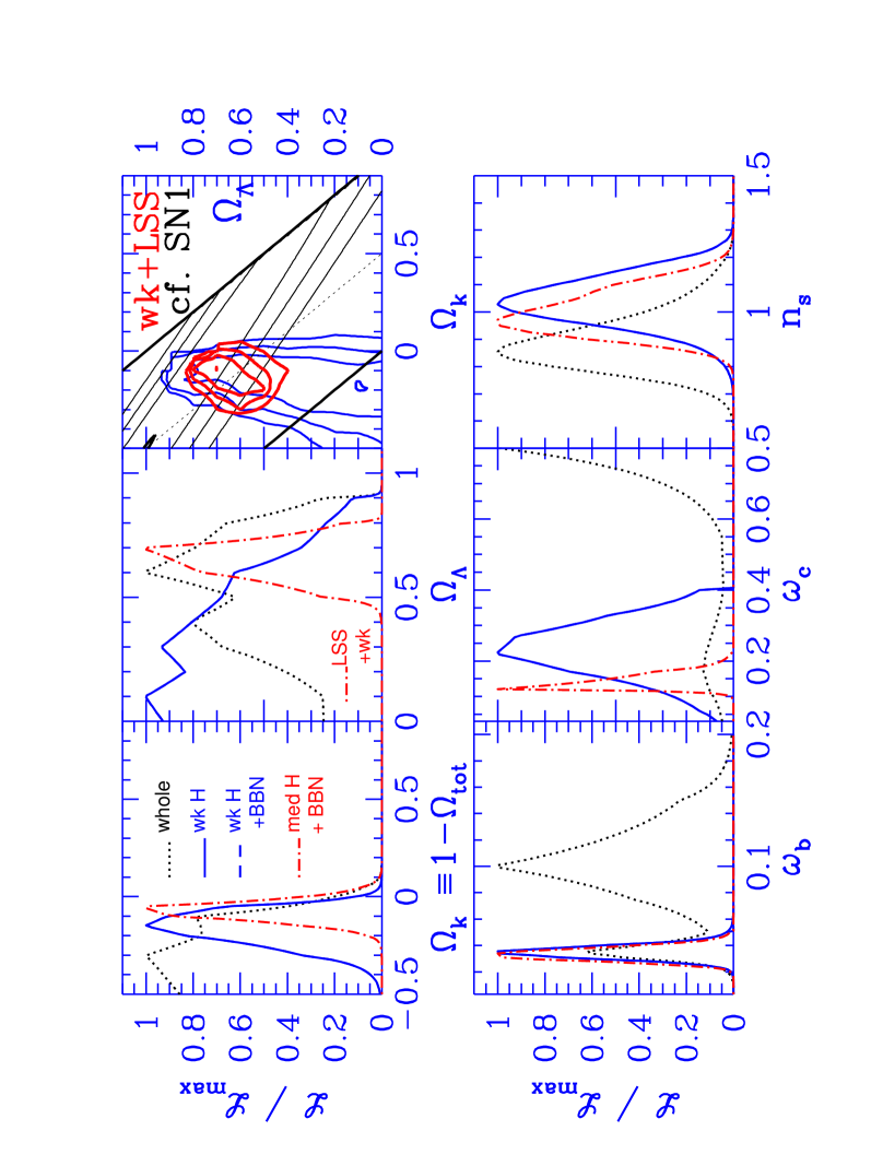
Figure 2: Likelihood functions for a subset of the priors used in Table 1. Panel 1 (top left) shows the likelihood for $\Omega_{k}\equiv 1-\Omega_{\rm{tot}}$; the full-database (P1, dotted line) prefers closed models, but reasonable priors (P2, dashed blue line; P4, solid blue line; P0, dot-dash red line; note that P2 and P4 lie on top of one another in every panel in this plot but are distinct in Figure 3) progressively move toward $\Omega_{k}=0$. We caution the reader against agressively interpreting any 2$\sigma$ effects. Likelihood curves for $\Omega_{\Lambda}$ are shown in panel 2 (top center). In panels 2 and 4-6, the cases and line types are as in panel 1, except that dot-dashed now denotes the weak+LSS prior, P5. With weak priors applied, there is no significant detection of $\Omega_{\Lambda}$ (P2 and P4, overlapping as solid blue line in all remaining $\mathcal{L}(x)$ panels). Only by adding the LSS prior is $\Omega_{\Lambda}$ localized away from zero (P5, red dot-dash in all remaining $\mathcal{L}(x)$ panels). Panel 3 (top right) shows the contour plot of $\Omega_{k}$ and $\Omega_{\Lambda}$, for which the first two panels are projections to one axis. The bold diagonal black lines mark $\Omega_{m}$=1 and $\Omega_{m}$=0. The blue contours are those found with the weak prior (P4), plotted at 1, 2, and 3$\sigma$contourerrors . Red contours are similarly plotted for the weak+LSS prior (P5). SN1a constraints are plotted as the lighter (black) smooth contours, and are consistent with the CMB contours at the $1\sigma$ level. Panel 4 (bottom left) shows the contours for $\omega_{b}$; the full database analysis results in a bimodal distribution with the higher peak concentrated at very high values. These high $\omega_{b}$ models are eliminated by the application of a weak $h$ prior or weak BBN prior (P2 and P4, overlapping as blue here). Panel 5 (bottom center) shows a localization of $\omega_{c}$ for the weak $h$ and BBN prior cases, but this is partially due to the effect of the database structure coupling to the $h$ and age priors. Only the LSS prior (P5, red dot-dash) allows the CMB to significantly constrain $\omega_{c}$. Panel 6 (bottom right) shows good localization and consistency in the $n_{s}$ determination once any priors are applied. The inflation-motivated $\Omega_{\rm{tot}}$=1 priors (P10, P11) give very similar curves localized around unity. See Figure 3 to see the effects of the database and priors on these curves.

References

- (1)
- (2) C. Bennett et al., Astrophys. J. 464, L1 (1996).
- (3) J. R. Bond, A. H. Jaffe and L. Knox, Astrophys. J., 533, 19, (2000). The bandpowers used to construct the radically compressed pre-Boomerang-LDB spectrum are listed there, except for the toco98 and mauskopf99 data which we have also included.
- (4) A. D. Miller, et al., Astrophys. J. 524, L1 (1999).
- (5) P. Mauskopf, et al., Ap. J. Letters, 536, L59, (2000).
- (6) L. Knox and L. Page, submitted to Phys. Rev. Lett., astro-ph/0002162 (2000).
- (7) e.g., J. R. Bond, G. Efstathiou and M. Tegmark, Mon. Not. R. Astron. Soc. 291, L33 (1997) and references therein; see also BJ98 for forecasts of LDB parameter extraction performance.
- (8) P. deBernardis et al., Nature 404, 955 (2000).
- (9) R. Durrer, A. Gangui, M. Sakellariadou, Phys. Rev. Lett. 76 579-582 (1996); e.g., B. Allen, et al., Phys. Rev. Lett. 79, 2624 (1997); U. Pen, N. Turok and U. Seljak, Phys. Rev. D 58, 023506 (1998); A. Albrecht, R. A. Battye and J. Robinson, Phys. Rev. D 59, 023508 (1999).
- (10) W. L. Freedman, astro-ph/9909076 (1999); J. R. Mould, et al., Astrophys J. 529, 786 (2000).
- (11) K. A. Olive, G. Steigman and T. P. Walker, submitted to Phys. Rep., astro-ph/9905320 (1999); D. Tytler, J. M. O’Meara, N. Suzuki and D. Lubin, submitted to Physica Scripta, astro-ph/0001318 (2000).
- (12) The spectra with massive neutrinos are quite similar to those without, and current data, including B98, will not be able to strongly constrain the value. When the LSS prior is added to the CMB data, however, the combination is quite powerful, e.g., BJ98 .
- (13) G. Efstathiou and J. R. Bond, Mon. Not. R. Astron. Soc. 304, 75 (1999).
- (14) Gravity waves (GW) can induce CMB anisotropy, and could have a separate tilt, , and an overall amplitude. They have little effect over the range of ’s that B98 is most sensitive to, but could have an important impact on the amplitude relative to COBE. To test the role that GW induced anisotropies would play, we have adopted the model used by BJ98 : for , we set and for , we allow no GW contribution. This presents a fixed alternative, reasonably motivated by inflation, without introducing new parameters. We have found that there is a negligible effect on the parameter determinations in Table 1; there is only a very slight migration upward in .
- (15) The specific values of the database variables used for this analysis are: ( 0.03, 0.06, 0.12, 0.17, 0.22, 0.27, 0.33, 0.40, 0.55, 0.8), ( 0.003125, 0.00625, 0.0125, 0.0175, 0.020, 0.025, 0.030, 0.035, 0.04, 0.05, 0.075, 0.10, 0.15, 0.2), (0, 0.1, 0.2, 0.3, 0.4, 0.5, 0.6, 0.7, 0.8, 0.9, 1.0, 1.1), (0.9, 0.7, 0.5, 0.3, 0.2, 0.15, 0.1, 0.05, 0, -0.05, -0.1, -0.15, -0.2, -0.3, -0.5), (1.5, 1.45, 1.4, 1.35, 1.3, 1.25, 1.2, 1.175, 1.15, 1.125, 1.1, 1.075, 1.05, 1.025, 1.0, 0.975, 0.95, 0.925, 0.9, 0.875, 0.85, 0.825, 0.8, 0.775, 0.75, 0.725, 0.7, 0.65, 0.6, 0.55, 0.5), (0, 0.025, 0.05, 0.075, 0.1, 0.15, 0.2, 0.3, 0.5)
- (16) U. Seljak and M. Zaldarriaga, Astrophys. J. 469, 437 (1996), http://www.sns.ias.edu/∼matiasz/CMB-FAST/cmbfast.html; A. Lewis, A. Challinor and A. Lasenby, astro-ph/9911177 (1999).
- (17) Apart from the 7 stated database parameters, we have allowed for an estimated 10% uncertainty in the calibration and the beam, which we determine simultaneously with the overall amplitude , by relaxing to the maximum likelihood value in these variables. We then determine the Fisher error matrix, assume that the variables are log-normally distributed, and evaluate a correction to the likelihoods appropriate for marginalization over these “intrinsic” variables. Including the marginalization correction makes little difference. We have also marginalized over bins that were used in creating the power spectrum but not in the analysis, since they are correlated.
- (18) The choice of measure is not important for strong localized peaks, but can potentially affect limits on poorly constrained variables and on those with complex likelihood functions. One can argue for logarithmic measures in (as we have used) and in and (which we have not used), and there are certainly philosophical alternatives to linear measures in and . Consider what happens when we turn the “whole database” likelihood curve of Figure 2 into a probability curve if we adopt a logarithmic rather than linear measure: the anomalous peak at 0.1 drops below the “cosmological peak” at 0.03; once weak priors are adopted, the 0.03 peak is all that is left and it is very stable to changing the measure. Changing measures usually moves peaks a small fraction of a , although the amount does depend upon relationships to correlated variables with large errors. The discreteness of our database is also a restriction on how accurately we can localize peaks. For example, our finest gridding in is 0.05 from 0.8 to 1.2, hence accurate localization better than half this spacing should not be expected. When projections are made, the available volume of models leads to effective priors as well hiddenpriors1 ; hiddenpriors2 .
- (19) The weak prior by itself actually focuses about 0.22, dropping to either side because of and age restrictions. Our data do constrain further, but not enough to claim a CMB determination beyond the prior until the LSS prior is included.
- (20) and have a prior probability dropping as drops and rises just because is positive. There is a physical effect that also favors the closed models when CMB is added. As varies, the sound speed lowers, the peak moves to higher , but can be mapped back to our observed by judiciously choosing an . moves the peak to lower which can also move back to the observed , but it is a smaller effect. If we had allowed , closed models could have done the same, further favoring because of the volume of models available.
- (21) e.g., M. White et al., Mon. Not. R. Astron. Soc. 283, pp107, (1996); K. Ganga et al., Astrophys. J. 484, 7 (1997); C. Lineweaver, Astrophys. J. 505, 69 (1998); ref. BJ98 ; G. Efsthathiou et al., Mon. Not. R. Astron. Soc. 303, pp47, (1998); S. Dodelson and L. Knox, Phys. Rev. Lett. 84, 3523 (2000); A. Melchiorri et al., Ap. J. Letters, 536, L63, (2000); M. Tegmark and M. Zaldarriaga, Astrophys. J., in press, astro-ph/0002091 (2000); M. Le Dour et al., submitted to Astron. and Astrophys., astro-ph/0004282 (2000).
- (22) J.R. Bond and A.H. Jaffe, Phil. Trans. R. Soc. London 357, 57 (1999), astro-ph/9809043.
- (23) The LSS prior is a slight modification of the one used in BJ98 . = is assumed to be distributed as a Gaussian smeared by a tophat distribution, with the first error indicating the 1- error on the Gaussian, and the second indicating the extent of the tophat about the mean. The constraint from power spectrum shapes involves a combination of spectrum tilt, , and a “scaling shape parameter” which is related to the horizon scale when the Universe passed from relativistic to matter dominance: =. Both priors were designed to generously encompass the observations, and so are “weak” to “medium” rather than “strong”, in the sense of Table 1.
- (24) The contours plotted at provide rough indicators of 1, 2, and 3 EB98 .
- (25) Riess et al., Astron. J. 116, 1009 (1998); S. Perlmutter et al., Astrophys. J. 517, 565 (1999).
- (26) Here are some sample correlation coefficients for the weak +BBN case of Table 1: it is relatively small between and other database variables but between and it is 86%. Similarly, as is evident from the contour map in Figure 2, and are correlated only at the 41% level, whereas and are correlated at the 96% level. Thus, for CMB work it is advantageous to use as a variable rather than , and hence this is what we plotted in Figure 2 rather than the more recognizable - plot. and have a 75% correlation, not surprising in view of that for .
- (27) For the P4 case, the best determined eigenmode (to ) is a combination of slope, amplitude and Thompson depth; next (to ) is predominantly , with a judicious negative contribution from , a combination orthogonal to the angular diameter distance degeneracy; the third eigenmode (to ) is mostly , with a little contribution from all other variables. The next three combinations are determined to . the worst () combination is one of and . Similar coefficients and accuracies hold for other priors, except for distortions in the strong BBN prior case.
- (28)