A critical-density closed Universe in Brans-Dicke Theory

Abstract

In a Brans-Dicke (BD) cosmological model, the energy density associated with some scalar field decreases as $\displaystyle a^{{-2}\left(\frac{\omega_{o}+{\frac{1}{2}}}{\omega_{o}+1}\right)}$ with the scale factor $a(t)$ of the Universe, giving a matter with an Equation of state $\displaystyle p=-\frac{1}{3}\left(\frac{2+\omega_{o}}{1+\omega_{o}}\right)\rho$. In this model, the Universe could be closed but still have a nonrelativistic-matter density corresponding to its critical value, $\Omega_{o}=1$. Different cosmological expressions, such as, luminosity distance, angular diameter, number count and ratio of the redshift tickness-angular size, are determined in terms of the redshift for this model.

1 Introduction

In the Friedman-Robertson-Walker (FRW) model, there are enough evidences that the Universe is flat, with a large component of negative pressure. This component was consider at first to be just the cosmological constant (or vacuum energy) (Tuner et al. 1984; Peebles 1984; Ostriker & Steinhard 1995; Liddle et al. 1996). Another possibility was to consider topological deffects (Vilenkin 1984), but, the one which has receiving a great deal of attention today, is related to a scalar field, $Q$, the so-called “quintessence” model or the QCDM model (Caldwell, Dave & Steinhardt 1998). This scalar field is characterized by a very negative pressure, i.e., $P_{Q}=w\rho_{Q}$, with $w\leq-1/3$.

Measurements of distant SNe Ia (at $z\sim 1$) indicate that the expansion of the Universe is in accelaration rather than deceleration (Perlmutter et al. 1998).

According to Garnavich et al. (1998) this is consistent with the existence of an unknown component for the energy density, which could be considered to correspond to the quintessence component. On the other hand, a test of the standard model, including spacetime geometry, galaxy peculiar velocities, structure formation, and early Universe physics, supports, in many of these cases, a flat Universe model with the presence of a cosmological constant (Peebles 1998). Specially, a model in which a short period of inflation occurs at a very early epoch in the evolution of the Universe.Most of these models predict that the total density parameter, $\Omega_{o}$, be unity.

Given the idea that the Universe could be described by a flat geometry, an interesting question to ask is whether this flatness could be due to a local effect. This sort of question has been considered in the literature ([Kamionkowski & Toumbas, 1996]). There, a $k=1$ model was taken into account, together with a total density parameter corresponding to $\Omega_{o}<1$. In this model, openness is obtained by considering a matter component whose equation of state is $\displaystyle p=-\frac{1}{3}\rho$. This sort of state of Equation has been reported in models in which topological defects, such as texture or tangled strings, are important components of the total energy of the Universe.

In this paper we analyse a FRW closed model, $k=1$, filled with dust and a effective density energy component characterized by a negative pressure, using the Brans-Dicke (BD) theory ([Brans & Dicke, 1961]) with a potential associated to the BD field. In particular, we investigate the conditions in order to have a model with positive curvature which mimics a flat universe at low redshift. This imply to determine the contributions of the scalar field $Q(t)$ and the BD field to the total energy density, which cancel the contribution due to curvature $\Omega_{ok}=-1/a_{0}H_{0}$. We should note that the obtained model is the generalization of the Einstein-de Sitter model ($k=0$) in the context of the BD theory. Our model is far from being realistic, since it gives an age for the universe,$t_{0}$, very close to $2H_{0}/3$, and a deceleration parameter, $q_{0}$, very close to $1/2$. These values, as we mentioned above, desagree with the measurements of distant supernovae. Nevertheless, we clearly pointed out that our proposal is to set the conditions under a closed universe mimics a flat universe in the BD theory. At the end of the following section we shall briefly discuss how in the BD theory a flat universe with negative pressures, presents acceleration in agreement with actual observations.

We studied this sort of model in a previous paper ([Cruz, del Campo & Herrera, 1998]), but that analysis was limited to the model’s intrinsic characteristics, such that the explicit determination of the scalar fields, $Q(t)$, its potential $V(Q)$ and the BD potential  $V(\Phi)$, where $\Phi$ represents the BD scalar field. In this paper we investigate the model’s cosmological characteristics, such that, the proper distance to the horizon, the luminosity distance, the angular size, the differential number of galaxies, and the ratio $(1/z)\delta z/\delta\theta$, where, all of these quantities are given as a function of the redshift $z$. We compare these parameters with that corresponding to the Einstein-de Sitter model.

We should note that our model, in the limit $\omega_{0}\rightarrow\infty$ and $\Phi=const$, gives rise to the $k=0$ Einstein-de Sitter model.

2 Characteristics of the model

Assuming homogeneity and isotropy, the FRW metric for a closed universe is

$$d\,{s}^{2}\,=\,\,d\,{t}^{2}\,-\,\,a(\,{t}\,)^{2}\,d\Omega_{k=1}^{2},$$ (1)

with $d\Omega_{k=1}^{2}$ representing the spatial line element asociated to the hypersurfaces of homogeneity, corresponding to a three sphere. $a(t)$ represents the scale factor, which together with the assumption that the $Q$ scalar field is homogeneous,i.e., $Q=Q({t})$, we obtain the fundamental field Equations of the BD model, given by (where the dots representing derivatives with respect to time $t$. We use units in which $c=\mathchar 2430\relax=1$ )

$$\hskip-99.58464pt\displaystyle H^{2}+H\left(\frac{\stackrel{{\scriptstyle\cdot}}{{\Phi}}}{\Phi}\right)=\frac{\omega_{o}}{6}\left(\frac{\stackrel{{\scriptstyle\cdot}}{{\Phi}}}{\Phi}\right)^{2}+$$

$$\hskip 99.58464pt\displaystyle\frac{8\pi}{3\Phi}\left(\rho_{M}+\rho_{Q}\right)-\frac{1}{a^{2}}+\frac{U\left(\Phi\right)}{6\Phi},$$ (2)

$$\hskip-99.58464pt\stackrel{{\scriptstyle\cdot\cdot}}{{\Phi}}+3H\stackrel{{\scriptstyle\cdot}}{{\Phi}}+\frac{\Phi^{3}}{2\omega_{o}+3}\frac{d}{d\Phi}\left(\frac{U(\Phi)}{\Phi^{2}}\right)=$$

$$\hskip 99.58464pt\frac{8\pi}{2\omega_{o}+3}\left[\rho_{M}+\left(1-3w\right)\rho_{Q}\right],$$ (3)

and

$$\stackrel{{\scriptstyle\cdot\cdot}}{{Q}}+3H\stackrel{{\scriptstyle\cdot}}{{Q}}=-\frac{\partial V(Q)}{\partial Q},$$ (4)

The condition describing a model mimicing a flat Universe is (Cruz, del Campo & Herrera 1998) given by

$$\hskip-99.58464pt\displaystyle\frac{d}{d\Phi}\left(\frac{U\left(\Phi\right)}{\Phi^{2}}\right)-\frac{1}{2\left(\omega_{o}+1\right)}\frac{U\left(\Phi\right)}{\Phi^{3}}$$

$$\hskip 99.58464pt\displaystyle+\frac{3}{\Phi_{0}^{2}(1+\omega_{o})}\left(\frac{\Phi_{0}}{\Phi}\right)^{2\left(2+\omega_{o}\right)}=0,$$ (5)

where $\Phi_{0}$ is the the actual value of the BD scalar field. Under these conditions Equation (2) and Equation (3)reduce to

$$H^{2}+H\left(\stackrel{{\scriptstyle\cdot}}{{\Phi}}/\Phi\right)=\frac{\omega_{o}}{6}\left(\stackrel{{\scriptstyle\cdot}}{{\Phi}}/\Phi\right)^{2}+\frac{8\pi}{3\Phi}\rho_{M},$$ (6)

and

$$\stackrel{{\scriptstyle\cdot\cdot}}{{\Phi}}+3H\stackrel{{\scriptstyle\cdot}}{{\Phi}}=\frac{8\pi}{2\omega_{o}+3}\rho_{M},$$ (7)

respectivelly. Equation (4) remains unaltered. Note that this set of equations mimics a flat ($\Omega_{m}=\Omega_{0}=1$) Universe.

Assuming that the matter content, $\rho_{M}$, is dominated by dust, i.e. $\rho_{M}\sim a^{-3}$, the solutions of Equations (6) and (7) are the well known power law solutions of a flat BD model, given by

$$a=a_{o}\left(\frac{t}{t_{o}}\right)^{\frac{2}{3}\left(\frac{\omega_{o}+1}{\omega_{o}+4/3}\right)},$$ (8)

and

$$\Phi(t)=\Phi_{o}\left(\frac{t}{t_{o}}\right)^{\left(\frac{2}{3\omega_{o}+4}\right)},$$ (9)

where $t_{o}$ is the current age of the Universe. Using the usual formula for the redshift $z$, $1+z=a_{o}/a$, we find that

$$t=\frac{2}{3}\left(\frac{\omega_{o}+1}{\omega_{o}+4/3}\right)H_{o}^{-1}\left(1+z\right)^{-\frac{2}{3}\left(\frac{\omega_{o}+4/3}{\omega_{o}+1}\right)},$$ (10)

where $H_{o}\equiv\sqrt{8\pi\rho_{M}^{o}/3\Phi_{o}}$, is the current Hubble constant taken as $H_{o}=100hkms^{-1}Mpc^{-1}$, with $h$ in the range $0.6\leq h\leq 0.8$ (Bureau, Mould & Staveley-Smith 1996). From Equation (10) we can obtain the age of the Universe, $\displaystyle t_{o}=\frac{2}{3}\left(\frac{\omega_{o}+1}{\omega_{o}+4/3}\right)H_{o}^{-1}=\left(\frac{\omega_{o}+1}{\omega_{o}+4/3}\right)t_{o}^{E}$, where $t_{o}^{E}$ is the Einstein-de Sitter value for the age of the Universe, given by $\frac{2}{3}H_{o}^{-1}$. At first glance, the factor appearing in $t_{o}$ seems to decrease the age of the Universe, due to $\displaystyle\left(\frac{\omega_{o}+1}{\omega_{o}+4/3}\right)\leq 1$. But, since $\omega_{o}\geq 500$ (Reasenberg et al. 1979), this factor will be small, and almost equal to one, and, therefore, we could use $t_{o}\simeq t_{o}^{E}$.

The growth of the Q-field is given by

$$\left(\frac{\stackrel{{\scriptstyle\cdot}}{{Q}}}{Q}\right)=2H_{o}\left(\frac{\omega_{o}+3}{\omega_{o}+1}\right)\left(1+z\right),$$ (11)

and its present value is then determined by the values of the Hubble constant, $H_{o}$, and the BD-parameter $\omega_{o}$. At large values of $\omega_{o}$ $(\omega_{o}\longrightarrow\infty)$ it becomes $\left(\stackrel{{\scriptstyle\cdot}}{{Q}}/Q\right)_{o}=2H_{o}$. On the other hand, the potential $V(Q)$ associated with this field is given by

$$V(Q)=M^{4}\left(\frac{M}{Q}\right)^{4\left(\frac{\omega_{o}+{\frac{1}{2}}}{\omega_{o}+1}\right)}$$ (12)

where $M$ is a free parameter.

Since $\displaystyle\rho_{Q}=\frac{3}{2}\left(\frac{\omega_{o}+1}{\omega_{o}+5/4}\right)V(Q)$ and the actual density parameter $\Omega_{Q}^{\omega_{o}}$ is defined by $\displaystyle\Omega_{Q}^{\omega_{o}}=\frac{8\pi\rho_{Q}^{o}}{3\Phi_{o}H_{o}^{2}}$, we find that $\displaystyle\Omega_{Q}^{\omega_{o}}=\left(\frac{\omega_{o}+1}{\omega_{o}+5/4}\right)\frac{4\pi M^{4}}{\Phi_{o}H_{o}^{2}}=\left(\frac{\omega_{o}+1}{\omega_{o}+5/4}\right)\Omega_{Q}$, where $\Omega_{Q}$ corresponds to the scalar field density parameter in Einstein-de Sitter’s model of the universe.

If we consider the same range for $\Omega_{Q}$ in our model, we find that this imposes a constrain on $M$. Since today it is required that $V(Q\approx M_{p\ell})\approx\rho_{m}\sim 10^{-47}{GeV^{4}}$, where $M_{p\ell}$ is the Planck mass, we obtain

$$M\sim\left(\rho_{m}M_{P\ell}^{4\left(\frac{\omega_{o}+{\frac{1}{2}}}{\omega_{o}+1}\right)}\right)^{\frac{\omega_{o}+1}{8\left(\omega_{o}+{\frac{3}{4}}\right)}}.$$ (13)

This gives $M\sim 10^{4}{GeV}$ for $\omega_{o}\sim 500$. This value is comparable to particle physics scales. We mention that the evolution of $Q$ and the values of $\Omega_{Q}$ today are very insensitive to the initial value of $Q$, due to its attractor solution (Zlater, Wang & Steinhardt 1998).

One point that needs to be taken into account in this kind of model is the fraction of the Universe in causal contact. To do so, we employ a comoving observer at coordinate $(r_{o}=0,\theta,\varphi)$ at time $t$. A light signal satisfies the geodesic equation of motion $ds^{2}=0$. Therefore, a light signal emitted from $\left(r_{1},\theta,\varphi\right)$ at time $t=0$, following the line $\theta=\phi=const.$, will reach the observer at time $t$

$$\int\limits_{o}^{t}\frac{dt^{\prime}}{a(t^{\prime})}=\int\limits_{o}^{r_{H}}\frac{dr}{\left(1-r^{2}\right)^{{\frac{1}{2}}}},$$ (14)

and because the proper distance to the horizon is

$$d_{H}(t)=\int\limits_{o}^{r_{H}}(g_{rr})^{\frac{1}{2}}dr,$$ (15)

it is found that

$$d_{H}(z)=a_{0}\,\frac{\alpha\left(\omega_{o},H_{o}\right)}{(1+z)}\left[1-\left(1+z\right)^{-\beta\left(\omega_{o}\right)}\right],$$ (16)

where $\displaystyle\alpha\left(\omega_{o},H_{o}\right)=\frac{2}{a_{o}H_{o}}\sqrt{\left(\omega_{o}+3/2\right)\left(\omega_{o}+4/3\right)}/\left(\omega_{o}+2\right)$ and $\displaystyle\beta\left(\omega_{o}\right)=\frac{1}{2}\left(\frac{\omega_{o}+2}{\omega_{o}+1}\right)$. In Fig. 1 we have plotted $d_{H}(z)$ as an function of $z$. In Einstein-de Sitter model we have nearly obtained the same curve.

Figure 1: This plot shows the horizon distance $d_{H}(z)$ (in unit of $H_{o}$) as a function of the redshift $z$, for the BD parameter $\omega_{o}=500$. The curve coincides with the corresponding to the Einstein-de Sitter model.

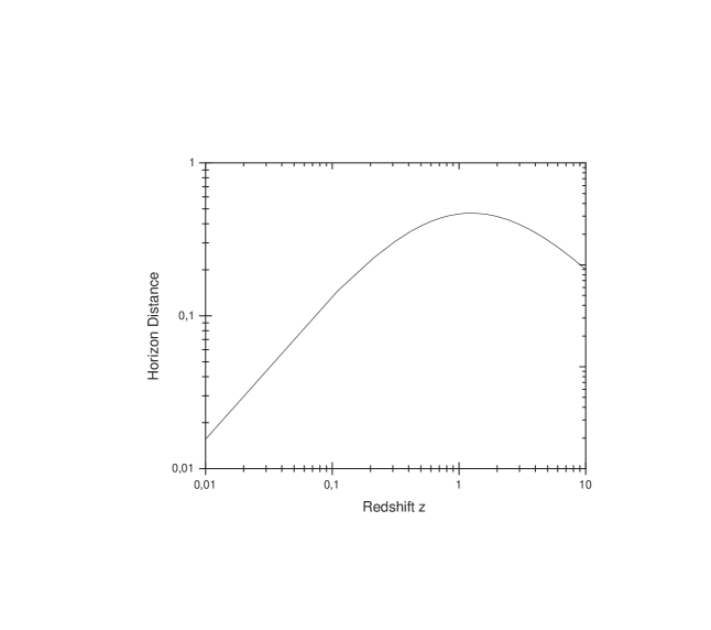
Since, $\omega_{o}\gg 1$, we can compare $d_{H}(z)$ in the BD theory with the corresponding expression in Einstein’s theory of general relativity (Einstein-de Sitter model). Expanding Equation (16) up to the first order in $1/\omega_{o}$, yields

$$d_{H}(z)\simeq d_{H}^{E}(z)+g(z,H_{o})(1/\omega_{o})+O(1/\omega_{o})^{2},$$ (17)

where $g(z,H_{o})$ becomes defined by

$$g(z,H_{o})=\frac{H_{o}^{-1}}{(1+z)}\left[\frac{7}{3}\left(\frac{1}{\sqrt{1+z}}-1\right)+\frac{\ell n\left(1+z\right)}{\sqrt{1+z}}\right],$$ (18)

and $d_{H}^{E}(z)$ represents the horizon distance in the Einstein-de Sitter model. This expression presents a maximum for $z\simeq 2$, and there, the difference, $\Delta d_{H}(z)\equiv d_{H}(z)-d_{H}^{E}(z)$, computed up to order $1/\omega_{o}$, becomes a maximum. Its value is not significant, since it is less than one percent.

In the following we determine the deceleration parameter $q_{o}$ for our model. This parameter is defined by $q_{o}=-\left(\ddot{a}/aH^{2}\right)_{o}$. By using the solution given by Eq. (8), we obtain that

$$q_{o}=\frac{1}{2}\left(\frac{\omega_{o}+2}{\omega_{o}+1}\right).$$ (19)

Note that we can write $q_{o}=\gamma\left(\omega_{o}\right)-1$, where $\gamma\left(\omega_{o}\right)$ is the inverse of the exponent in the expression of the scale factor $a(t)$, i.e. $\displaystyle\gamma\left(\omega_{o}\right)=\frac{3}{2}\left(\frac{\omega_{o}+4/3}{\omega_{o}+1}\right)$. If we consider the lower bound for $\omega_{o}$, i.e. $\omega_{o}\simeq 500,$ we find that the deceleration parameter has a value close to one half, as it should be in the Einstein-de Sitter model

Following the approach done by Uehara and Kim (1982), we may write directly an expression for the deceleration parameter $q_{o}$ given by

$$q_{o}=\epsilon_{o}+\frac{\omega_{o}}{3}\epsilon_{o}^{2}+\frac{1}{2}\left(\frac{\omega_{o}+3}{\omega_{o}+3/2}\right)\Omega_{m},$$ (20)

Notice that this factor is related to the present rate of change of the Newton’s gravitational constant expressed by $\displaystyle\left(\stackrel{{\scriptstyle\cdot}}{{G}}/G\right)_{o}=\mid\frac{\dot{\Phi}}{\Phi}\mid_{0}$, since $\displaystyle G(\Phi)=\frac{1}{\Phi}$.

The contribution to the deceleration parameter in Equation (20) is small, since its experimental upper limit is given by $\left(\stackrel{{\scriptstyle\cdot}}{{\Phi}}/\Phi\right)_{o}\mathchar 14382\relax 10^{-10}yr^{-1}$ (Helling et al. 1983; Dickey, Newhall & Williams 1989; Shapiro 1989). More recent, measurements on white dwarfs, have decreased the upper limit to $\displaystyle\mid\frac{\dot{G}}{G}\mid_{0}<10^{-11}yr^{-1}$ (García-Berro et al. 1995). Still smaller upper limits for this quantity have been reported (Müler et al. 1991), where lunar laser-ranging studies of the moon’s Earth orbit yields $\displaystyle\mid\frac{\dot{G}}{G}\mid_{0}<10^{-13}yr^{-1}$. Since $\epsilon_{0}\ll 1$, we can write, $\displaystyle q_{o}\simeq\frac{1}{2}\left(\frac{\omega_{o}+3}{\omega_{o}+3/2}\right)\Omega_{m}$, which becomes exactly one half the result of Einstein-de Sitter’s theory.

At this point we would like to mention that it is possible to describe in the same spirit, the situation in which the model represents an accelerating flat universe, i. e. a model in Brans-Dicke theory in which now $\Omega_{0}=\Omega_{m}+\Omega_{\lambda}=1$. But, as we will see, this case becomes quite complicate to handle. We shall postpone the details of these studies for the near future. We shall restrict ourselves here to give a brief description of this situation. In this case the condition (5) becomes

$$\hskip-99.58464pt\displaystyle\frac{d}{d\Phi}\left(\frac{U\left(\Phi\right)}{\Phi^{2}}\right)+(1-3w)\frac{U\left(\Phi\right)}{\Phi^{4}}$$

$$\hskip 71.13188pt\displaystyle=3(1-w)\frac{\lambda}{\Phi^{2}}+3(1-3w)\frac{1}{\Phi^{2}\,a^{2}(\Phi)}.$$ (21)

If we want to get an explicit form of the Brans-Dicke scalar potential, $U(\Phi)$, we need to know the scale factor $a$ as a function of the Brans-Dicke scalar field $\Phi$. In order to do this, we consider the set of basic field equations

$$H^{2}+H\left(\stackrel{{\scriptstyle\cdot}}{{\Phi}}/\Phi\right)=\frac{\omega_{o}}{6}\left(\stackrel{{\scriptstyle\cdot}}{{\Phi}}/\Phi\right)^{2}+\frac{8\pi}{3\Phi}\rho_{M}+\frac{\lambda}{3},$$ (22)

and

$$\stackrel{{\scriptstyle\cdot\cdot}}{{\Phi}}+3H\stackrel{{\scriptstyle\cdot}}{{\Phi}}=\frac{8\pi}{2\omega_{o}+3}\rho_{M}+\frac{2\lambda}{2\omega_{o}+3}\Phi,$$ (23)

(together with equation (4)) that can be solved exactly (Uehara and Kim 1982). The solution for $\lambda>0$ is given by

$$\hskip-99.58464pt\displaystyle a(t)=a_{o}\left[A\cosh\left(\eta\triangle t\right)-\frac{4\pi}{\lambda}\right]^{\alpha(\omega_{o})}$$

$$\hskip 28.45274pt\times\left[\frac{B\tanh\left(\frac{1}{2}\eta\triangle t\right)-\sqrt{(4\pi/\lambda)^{2}-A^{2}}}{B\tanh\left(\frac{1}{2}\eta\triangle t\right)+\sqrt{(4\pi/\lambda)^{2}-A^{2}}}\right]^{\beta(\omega_{o})},$$ (24)

where,$\eta^{2}$, $A^{2}$, $B$, $\alpha(\omega_{o})$ and $\beta(\omega_{0})$ are given by $\displaystyle{\frac{2(4+3\omega_{o})}{3+2\omega_{o}}}$, $\displaystyle{\left[\frac{4\pi}{\lambda}\right]]^{2}-\frac{3}{2\lambda}\frac{1}{4+3\omega_{o}}\left[\frac{\Phi_{o}}{\rho_{o}}\right]^{2}\left[(1+\omega_{o})\epsilon_{o}+H_{o}\right]^{2}}(>0)$,
$\displaystyle{\frac{4\pi}{\lambda}+A}$, $\displaystyle{\frac{1+\omega_{o}}{4+3\omega_{o}}}$ and $\displaystyle{\frac{1}{4+3\omega_{o}}\sqrt{\frac{3+2\omega_{o}}{3}}}$, respectively. The interval of time, $\triangle t=t-t_{c}$, is related to $\displaystyle{t_{c}=-\frac{2}{\eta\sqrt{\lambda}}\left[\frac{4\pi/\lambda-A}{\frac{4\pi}{\lambda}+A}\right]}$.

Expressions (24) together with equation (22) allow us to determine the scalar field $\Phi$ as a function of time. Thus, in principle, we could get the scale factor as a function of the Brans-Dicke scalar field.

We should note that the deceleration rate $q_{o}$ becomes in this case

$$q_{o}=\epsilon_{o}+\frac{\omega_{o}}{3}\epsilon_{o}^{2}+\frac{1}{2}\left(\frac{\omega_{o}+3}{\omega_{o}+3/2}\right)\Omega_{m}-\frac{2\omega_{o}}{2\omega_{o}+3}\Omega_{\lambda},$$ (25)

with $\Omega_{\lambda}$ defined by $\displaystyle{\frac{\lambda}{3H^{2}_{o}}}$. Notice that if the cosmological constant contribution to the total density parameter is significant, in agreement with the Supernova observations, the deceleration parameter becomes negative and thus the universe will show an acceleration. We stop here this analysis and, as we have mentioned above, we shall describe in more details this situation in near future.

In going back to our simple Einstein-de Sitter-like model in BD theory, we discuss in the following some kinematical properties.

3 Kinematics of the model

3.1 Luminosity Distance-Redshift

The “luminosity distance” is defined as the ratio of the emitted energy per unit time, ${\cal L}$, and the energy received per unit time ${\cal F}$

$$d_{L}^{2}=\frac{{\cal L}}{4\pi{\cal F}}$$ (26)

In the absence of an expansion, the luminosity distance is simply the physical distance to the source. In closed FRM cosmology, the luminosity distance to a source at coordinate $\left(r_{1},\theta,\phi\right)$ is, assuming for convenience that the observer is located at $r=0$,

$$d_{L}^{2}(z)=a_{0}^{2}r_{1}^{2}(z)(1+z)^{2},$$ (27)

The factor $a_{0}^{2}r_{1}^{2}$ in this expression is nothing but the “inverse square law”, since a two-sphere surrounding the source encompassing the observer has an area equal to $4\pi a_{0}^{2}r_{1}^{2}(z)$. The factor $(1+z)^{2}$ appears due to the redshift of the radiation between the time of emission and the time of detection. The parameter $r_{1}$ is determined by the expression

$$\int\limits_{o}^{r_{1}(z)}\frac{dr}{\sqrt{1-r^{2}}}=\frac{1}{H_{o}}\int\limits_{o}^{z}\frac{dz}{E(z)},$$ (28)

where $E(z)$ is given by

$$E(z)=\frac{\left(1+z\right)^{\gamma\left(\omega_{o}\right)}}{a_{o}H_{o}\beta\left(\omega_{o}\right)\alpha\left(\omega_{o},H_{o}\right)}.$$ (29)

Thus, we find for the Luminosity distance-redshift relation

$$d_{L}(z)=a_{o}(z+1)\sin\left\{\alpha\left(\omega_{o},H_{o}\right)\left[1-(1+z)^{-\beta(\omega_{o})}\right]\right\}.$$ (30)

Fig. 2 shows how the luminosity distance, $d_{L}\left(z\right)$, changes with redshift parameter $z$, for Einstein-de Sitter model (dotted line) and BD closed model (solid line) . From this Figure we observe that the BD-theory begins to differ from Einstein-de Sitter’s theory at $z\simeq 100$. If we take the value for the redshift $z$ corresponding to the value associated to the last scattering surface, i.e. $z\equiv z_{LS}\simeq 1.100$, the luminosity distance in Einstein-de Sitter’s theory differs approximately from its analogous expression in the BD theory by a few percentage points.

Figure 2: Plot of the luminosity distance $d_{L}(z)$ (in unit of $H_{o}$) as a function of the redshift $z$. The continuous line corresponds with $\omega_{o}=500$ (BD theory) and the dotted line represents the luminosity distance in the Einstein-de Sitter model.

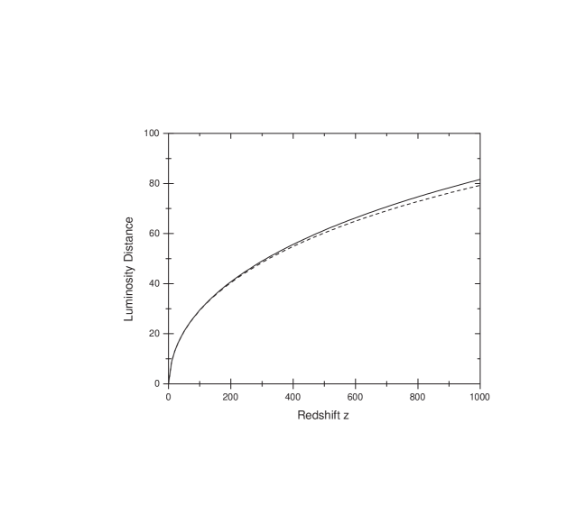
Note that for small $z$, Equation (30) yields

$$H_{o}d_{L}(z)=z+\frac{1}{2}\left(1-\beta\left(\omega_{o}\right)\right)z^{2}+o(z^{3}),$$ (31)

where we have rescaled the luminosity distance by a factor of $a_{o}H_{o}\beta\left(\omega_{o}\right)\alpha\left(\omega_{o},H_{o}\right).$ The first term of this expression is nothing but the Hubble law, and from the second term, we can read the $q_{o}$ parameter, $\displaystyle q_{o}=\beta\left(\omega_{o}\right)=\frac{1}{2}\left(\frac{\omega_{o}+2}{\omega_{o}+1}\right)$, which coincides with the result obtained above.

Also, from Equation (30) we can use the apparent bolometric magnitude $m(z)$ of a standard candle (with $M$ equal to the absolute bolometric magnitude) as a function of the redshifts

$$m(z)=M+5log[d_{L}(z)]+25.$$ (32)

If we define $D_{L}(z)\equiv H_{o}d_{L}(z)$, then we obtain, from the latter Equation

$$m(z)={\cal M}+5log[D_{L}(z)],$$ (33)

where ${\cal{M}}\equiv M-5log(H_{o})+25$, is the magnitude ”zero point”, which can be determined observationally. Hamuy et al. (1996) have determined the value ${\cal{M}}=-3.17\pm 0.03$ using 18 supernovae discovered by the Calán/Tololo researchers. This value is supposed to be independent of the redshift $z$. Therefore, if we take two different values for the redshift, we can obtain a variation of the apparent bolometric magnitude which is given by $\Delta m\left(z_{2},z_{1}\right)\equiv 5\log\left[d_{L}(z_{2})/d_{L}(z_{1})\right]$, or explicitly

$$\hskip-156.49014pt\Delta m\left(z_{2},z_{1}\right)=5\log$$

$$\hskip 22.76228pt\displaystyle\left\{\frac{\left(1+z_{2}\right)\sin\left[\alpha\left(\omega_{o},H_{o}\right)\left(1-\left(1+z_{2}\right)^{-\beta\left(\omega_{o}\right)}\right)\right]}{\left(1+z_{1}\right)\sin\left[\alpha\left(\omega_{o},H_{o}\right)\left(1-\left(1+z_{1}\right)^{-\beta\left(\omega_{o}\right)}\right)\right]}\right\}.$$ (34)

This expression could be used to restrict the value of the BD parameter $\omega_{o}$.

By using the values $z_{1}=0.5$ and $z_{2}=1.0$, we find the $\Delta m$  increases monotonically with the BD-parameter $\omega_{o}$. When this parameter reaches a value close to $\omega_{o}\simeq 20$, the growth of $\Delta m$ with respect to $\omega_{o}$ increases, but slowly now, approaching asymptotically a limiting value. At $\omega_{o}=500$ this difference yields the value $\Delta m\simeq 3.32$.

On the other hand, if we consider the values specified by Goobar & Perlmutter (1995) in which the apparent magnitude (R-band) was $m_{R}=22.17\pm 0.05$ at redshift $z=0.5$ and $m_{R}=25.20\pm 0.05$ at redshift $z=1.0$, we obtain $\Delta m_{R}=3.03\pm 0.05$. This value represents a similar order of magnitude as that obtained for $\omega_{o}=500$.

3.2 The Angular diameter-redshift

The angular diameter distance $d_{A}$ between a source at redshift $z_{2}$ and $z_{1}<z_{2}$ is defined by

$$d_{A}\left(z_{1},z_{2}\right)=\frac{a_{o}\sin\left[\Delta\chi\left(z_{1},z_{2}\right)\right]}{\left(1+z_{2}\right)}$$ (35)

where $\Delta\chi\left(z_{1},z_{2}\right)$ is the polar-coordinate distance between a source at $z_{1}$ and another at $z_{2}$, in the same line of sight

$$\Delta\chi(z_{1},z_{2})=\alpha\left(\omega_{o},H_{o}\right)\left[\left(1+z_{1}\right)^{-\beta\left(\omega_{o}\right)}-\left(1+z_{2}\right)^{-\beta\left(\omega_{o}\right)}\right]$$ (36)

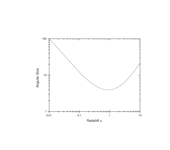
The corresponding angular size of an object of proper length $\ell$ at a redshift $z$ results in $\theta\left(z\right)\simeq\ell/d_{A}\left(0,z\right)$, which becomes (in units of $\ell H_{o}$)

$$\Theta\left(z\right)=\frac{1}{a_{o}H_{o}}\frac{\left(1+z\right)}{\sin\left\{\alpha\left(\omega_{o},H_{o}\right)\left[1-\left(1+z\right)\right]^{-\beta\left(\omega_{o}\right)}\right\}}$$ (37)

Fig. 3 shows the plot of $\Theta$ as a function of $z$ in Einstein-de Sitter’s theory and the BD theory with $\omega_{o}=500$. These two theories coincide in the $0\leq z\simeq z_{LS}$. At $z=z_{LS}$, it is found that in the first approximation of $1/\omega_{o}$, their difference is $\Delta\Theta\equiv\Theta_{BD}-\Theta_{E}\sim 147\left(1/\omega_{o}\right)$, for any large value of $\omega_{o}$. In this plot, we have taken $a_{0}H_{0}=\sqrt{2/5}$ [Kamionkowski & Toumbas, 1996].

Figure 3: This plot show the angular size (in unit of $lH_{o})$ as a function of the redshift $z$, as expressed by Equation (37) for the case $\omega_{o}=500$. We should mention that the corresponding curve for the Einstein-de Sitter model is indistinguishable in the range $0\leq z\leq z_{LS}$.

3.3 The number count-redshift

The number of galaxies in a comoving volume element in an angular solid area $d\Omega$ with redshift between $z$ and $z+dz$ is sensitive to the number of galaxies, $n$, in a comoving volume element $dV_{c}$ and the spatial curvature:

$$dN_{gal}=ndV_{c}=n\frac{r^{2}}{\left(1-r^{2}\right)^{{\frac{1}{2}}}}drd\Omega$$ (38)

¿From this relation we can write the differential number of galaxies per steradian per unit redshift,

$$\frac{dN_{gal}}{dzd\Omega}\left(z\right)=\frac{n\,a_{o}^{2}\,\sin^{2}\left[\Delta\chi\left(z\right)\right]}{H_{o}E(z)}$$ (39)

Using the expression for $\Delta\chi(z)$ from Equation 36 and $E(z)$ from Equation (29), we obtain

$$\hskip-99.58464pt\displaystyle\frac{dN_{gal}}{dzd\Omega}\left(z\right)=n\,a_{o}^{3}\alpha(\omega_{o},H_{o})\beta(\omega_{o})\times$$

$$\hskip 42.67912pt\displaystyle\frac{\sin^{2}\left\{\alpha(\omega_{o},H_{o})\left[1-\left(1+z\right)^{-\beta\left(\omega_{o}\right)}\right]\right\}}{\left(1+z\right)^{\gamma\left(\omega_{o}\right)}}.$$ (40)

In Fig. 4 we have plotted the number-redshift relation (given by Equation (39)), for $\omega_{o}=500$. Here, we have confirmed that, for a large range of the redshift z, the function of the number of galaxies per unit of steradian per unit redshift in Einstein-de Sitter’s model becomes almost indistinguishable from its similar expression in the BD-theory.

Figure 4: The differential number of galaxies per unit redshift per steradian in units of $nH_{o}^{-3}$ for the BD parameter $\omega_{o}=500$. At a low redshifts these differential numbers rapidly approach zero.

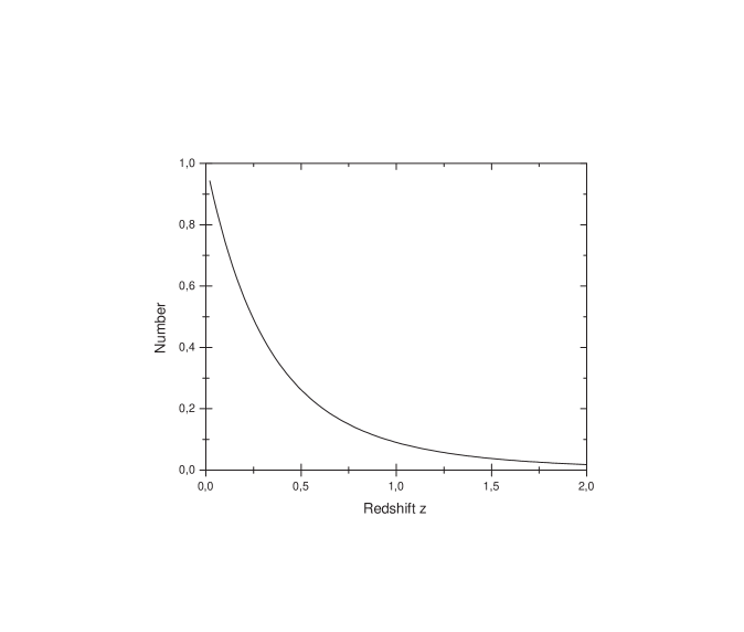
For small redshift one obtaines

$$\frac{dN_{gal}}{dz\,d\Omega}\left(z\right)\simeq n\,\left(a_{o}\,\alpha(\omega_{o},H_{o})\,\beta(\omega_{o})\right)^{3}z^{2}+O\left(z^{3}\right)\,.$$ (41)

This expression indicates that, for small redshift, the slope in the plot $\displaystyle\frac{dN_{gal}}{dz\,d\Omega}$ v/s $z^{2}$ could provide some information about the $\omega_{o}$ BD parameter, assuming that the present value of the Hubble constant $H_{o}$ is known. This, in principle, could be checked by the corresponding observations.

3.4 The ratio of the redshift thickness-angular size

The redshift thickness $\delta z$ and the angular size $\delta\theta$ of a spherical structure that grows with the expansion of the Universe have a dependence on $z$ given by

$$\frac{1}{z}\frac{\delta z}{\delta\theta}(z)=a_{o}H_{o}\frac{E(z)\sin\left[\Delta\chi(z)\right]}{z},$$ (42)

or explicitly,

$$\frac{1}{z}\frac{\delta z}{\delta\theta}(z)=\frac{\left(1+z\right)^{\gamma(\omega_{o})}\sin\left\{\alpha\left(\omega_{o},H_{o}\right)\left[1-\left(1+z\right)^{\beta(\omega_{o})}\right]\right\}}{a_{o}H_{o}\alpha\left(\omega_{o},H_{o}\right)\beta(\omega_{o})z}$$ (43)

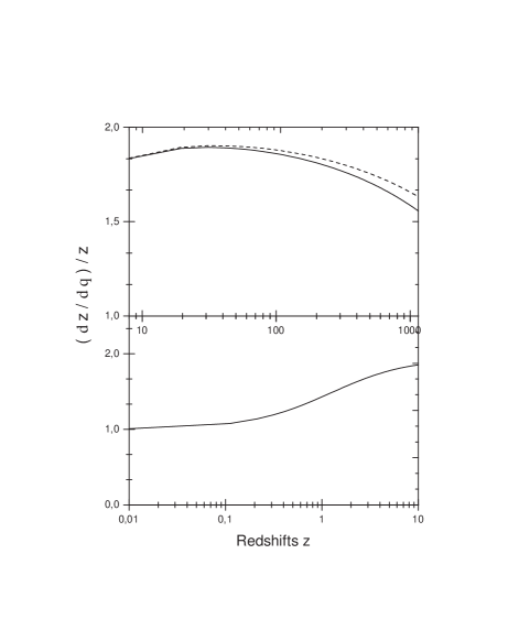
Fig. 5 (lower panel) shows how $\displaystyle\frac{1}{z}\frac{\delta z}{\delta\theta}$ changes with redshift $z$ in the BD-theory, for $\omega_{o}=500$. We see that, in the range of $0\leq z\leq 10$, there is no difference when it is compared with its analogous expression in Einstein-de Sitter model. However, at large redshift i.e. $z\equiv z_{LS}\sim 1.100$, their difference becomes significant, as we can see from Fig. 5 (upper panel). Thus, the two expressions differ at large redshift values.

Figure 5: In the lower panel we plot $\left(\delta z/\delta\theta\right)/z$ as a function of $z$ in BD theory (for $\omega_{o}=500$) at low redshift. In upper panel we have plotted $\left(\delta z/\delta\theta\right)/z$ in Einstein-de Sitter (dashed line) and BD theories (continous line) for $z>10$. Note that these two curves become different at very high redshift.

4 Conclusions

We have studied a model in which the “quintessence” component was included. In this model we have chosen a Universe with closed topology $\left(k=1\right)$ in the BD theory, and we have added a scalar potential for the BD-scalar field. The quintessence contribution to the matter component was fine tuned to exactly cancel the curvature term (with the help of the BD scalar potential) in the corresponding field Equations.

Under these conditions, different cosmological expressions were calculated as a function of the redshift $z$. For instance, the luminosity distant, the angular diameter, the number count and ratio of the redshift thickness-angular size. All these quantities were compared with their analogous expression related to Einstein-de Sitter model which seems flat at low redshift. In some cases (Luminosity distance and the ratio of the redshift thickness-angular size), the corresponding expressions become distinguishable at a high enough redshift. At that redshift, these differences are difficult to be directly detected . Perhaps, if we consider other observational facts, such as, the anisotropy of the cosmic microwave background radiation, we might say something about these differences, and use these results for establishing a limit for the BD parameter, $\omega_{o}$, since the two theories differ in the value of this parameter.

References

- [Brans & Dicke, 1961] Brans, C., & Dicke, R.H. 1961, Phys. Rev., 124, 925.
- [Bureau, Mould & Staveley-Smith, 1996] Bureau, M., Mould, J.R., & Staveley-Smith, L. 1996, Ap.J.,463, 60; T. Kundić, et al. 1997, Ap.J. 482, 75; J.L. Tonry, J.P. Blakeslee, Ajhar, E.A.,& Dressler, A. 1997, Ap.J. 475, 399.
- [Caldwell, Dave & Steinhardt, 1998] Caldwell, R. Dave, R. & Steinhardt, P.J. 1998, Phys. Rev. Lett., 80, 1582.
- [Cruz, del Campo & Herrera, 1998] Cruz, N., del Campo, S. & Herrera, R. 1998, Phys. Rev. D, 58, 123504.
- [Dickey, Newhall, & Williams, 1989] Dickey, J., Newhall, X. & Williams, J. 1989, Adv. Space. Res., 9, 75.
- [Falco, Kochanek & Muñoz, 1998] Falco, E.E., Kochanek, C.S., & Muñoz, J.A. 1998, Ap.J. 494, 47.
- [García-Berro et al. 1995] García-Berro, E. Hernaz, M. Isern, J. & Mochkovich, R. 1995, M.N.R.A.S. 227, 801.
- [Goobar & Perlmutter, 1995] Goobar, A. & Perlmutter, S. 1995, Ap.J. 450, 14.
- [Helling et al., 1983] Helling, R. W., et al. 1983, Phys. Rev. Lett., 51, 1609.
- [Kamionkowski & Toumbas, 1996] Kamionkowski, M. & Toumbas, N. 1996, Phys. Rev. Lett., 77, 587.
- [Liddle et al, 1996] Liddle, A.R., et al. 1996, M.N.R.A.S. 282, 281.
- [Müler et al, 1991] Müler, J., Schneider, M., Soffel, M. & Ruder, H. 1991, Ap.J. 382, L101.
- [Ostriker & Steinhard, 1995] Ostriker, J.P & Steinhardt, P. J. 1995, Nature, 377, 600.
- [Peebles, 1984] Peebles, P.J.E. 1984, Ap.J. 284, 439.
- [Peebles, 1998] Peebles, P.J.E., 1998, astro-ph/9806201.
- [Perlmutter, 1998] Perlmutter, S., et al. 1998, Nature, 391, 51.
- [Reasenberg et al, 1979] Reasenberg, R.D., et al. 1979, Ap.J. 234, 219.
- [Shapiro, 1989] Shapiro, I. 1990, General Relativity and Gravitation, ed. N. Ashly, D. Bartlett & W. Wyss (Cambridge: Cambridge Univ. Press).
- [Turner et al, 1984] Turner, M.S. Steigman, G. & Krauss, L. 1984, Phys. Rev. Lett., 52, 2090.
- [Turner & White, 1997] Turner, M.S. & White, M. 1997, Phys. Rev. D, 56, R4439.
- [Vilenkin, 1984] Vilenkin, A., 1984, Phys. Rev. Lett., 53, 1016.
- [Zlatev, Wang & Steinhardt, 1998] Zlatev, I. Wang, L. & Steinhardt, P.J. 1999, Phys. Rev. Lett. 82, 896.