Topological defects: fossils of an anisotropic era?

Abstract

We consider the evolution of domain walls produced during an anisotropic phase in the very early universe, showing that the resulting network can be very anisotropic. If the domain walls are produced during an inflationary era, the network will soon freeze out in comoving coordinates retaining the imprints of the anisotropic regime, even though inflation makes the universe isotropic. Only at late times, when the typical size of the major axis of the domain walls becomes smaller than the Hubble radius, does the network evolve rapidly towards isotropy.

Hence, we may hope to see imprints of the anisotropic era if by today the typical size of the major axis of the domain walls is of the order of the Hubble radius, or if the walls re-entered it only very recently. Depending on the mass scale of the domain walls, there is also the possibility that they re-enter at earlier times, but their evolution remains friction-dominated until recently, in which case the signatures of the anisotropic era will be much better preserved. These effects are expected to occur in generic topological defect models.

I Introduction

It is well know that the ‘Hot Big Bang’ model [1], despite its numerous successes, is plagued by a number of ‘initial conditions’ problems, of which the horizon, flatness and unwanted relic ones are the best known. The standard way to solve them is to invoke an epoch of cosmological inflation [2, 3, 4], a relatively brief period of exponential (or quasi-exponential) cosmological expansion. The way inflation solves these problems is, loosely speaking, by erasing all traces of earlier epochs and re-setting the universe to a rather simple state. Indeed, inflation is so efficient in this task that a number of people have wondered if one can ever hope to probe the physics of a pre-inflationary epoch.

There are, however, a small number of possible pre-inflationary relics. For example, the recent work by Turok and collaborators [5] shows that curvature can, in some sense, survive inflation. Another class of inflationary survivors are topological defects [6], formed at phase transitions either before or during inflation [7, 8, 9]). It is known (see, e.g. [1, 3, 10]) that one needs about 20 e-foldings of inflation to solve the monopole problem. One can reverse the argument and say that monopoles can survive about 20 e-foldings of inflation. The inflationary epoch itself will obviously push the monopoles outside the horizon, but the subsequent evolution of the universe tends to make them come back inside, so if the inflationary epoch is not too long they can still have important cosmological consequences.

Cosmic strings are even more successful, being able to survive about 50 e-foldings. The reason for this difference is that their non-trivial dynamics [11, 12, 13, 10] makes them come back inside the horizon faster than one might naively have expected. The above two numbers are typical, but there are specific models where defects can survive even longer. One example is that of open inflation scenarios [14]. In this case the universe undergoes two different inflationary epochs—roughly speaking, a period of ‘old inflation’ followed by one of ‘new inflation’. As pointed out by Vilenkin [15], one can expect that defects will form between the two inflationary epochs. In this case, a collaboration [10] including the present authors has recently shown that not only will cosmic strings survive the entire second inflationary epoch, regardless of how long it lasts, but they will in fact be back inside the horizon by the time of equal matter and radiation densities. In such models, monopoles can survive up to about 30 e-foldings.

Now, given that defects seem to be so successful surviving inflation, and that one expects them to be frozen out while they are outside the horizon, one can think of a further interesting possibility. For the best-studied case of cosmic strings, it is well known that the scaling properties of the network depend on the background cosmology [11, 12, 13]. Moreover, in some cases (typically when their evolution is friction-dominated) they can retain a ‘memory’ of the initial conditions, or the general properties of the cosmology in which they find themselves at early times, for quite a large number of orders of magnitude in time [11, 13]. It is therefore conceivable that if such an imprint of an early cosmological epoch is retained by a defect network which manages to survive inflation, we might still be able to observe it today.

We believe that this is a general feature of defect models, and a number of non-trivial pieces of information about the very early universe can probably be preserved in this way. In the present paper we will restrict ourselves to a simple example. We will discuss the possibility of a domain wall network retaining information about an early anisotropic phase of the universe. There are very strong constraints [16] on the mass of domain walls formed after inflation, due to the fact that their density decays more slowly than the radiation and matter densities. However, these can be evaded by walls forming before or during inflation. In a subsequent paper, we will discuss the more interesting, but also more complicated, case of cosmic strings.

The plan of the paper is as follows. In section II we briefly describe our background (Bianchi I) cosmology and the basic evolutionary properties of the domain walls. In particular, we focus on the approach to isotropy during inflation, which is discussed through both analytic arguments and numerical simulations. We emphasise that these simulations do not include the defects. However, they serve an important purpose, as they are used in the subsequent discussion to show that the timescale needed for isotropization is compatible with the ‘survival’ on anisotropic defect networks.

We provide a description of our numerical simulations of domain wall evolution in section III. These are analogous to those of Press, Ryden & Spergel [17], and the interested reader is referred to this paper for a more detailed discussion of some relevant numerical issues. Here defect networks are evolved in an isotropic, matter-dominated (ie, post-inflationary universe), and their main purpose is to show that isotropic and anisotropic networks will evolve in different ways, so two such networks can in principle be observationally distinguished as they re-enter the horizon. Our main results are presented and discussed in section IV, and finally we present our conclusions and discuss future work in section V.

Throughout this paper we will use fundamental units in which $c=1$.

II Evolution equations for domain walls

We consider the evolution of a network of domain walls in a k=0 anisotropic universe of Bianchi type I with line element [18]:

$$ds^{2}=dt^{2}-X^{2}(t)dx^{2}-Y^{2}(t)dy^{2}-Z^{2}(t)dz^{2}$$ (1)

where $X(t)$,$Y(t)$ and $Z(t)$ are the cosmological expansion factors in the $x$, $y$ and $z$ directions respectively, and $t$ is the physical time. The dynamics of a scalar filed $\phi$ is determined by the Lagrangian density,

$${\cal L}=-{1\over{4\pi}}\left({1\over 2}\phi_{,\alpha}\phi^{,\alpha}+V(\phi)\right),$$ (2)

where we will take $V(\phi)$ to be the generic $\phi^{4}$ potential with two degenerate minima given by

$$V(\phi)=V_{0}\left({\phi^{2}\over\phi_{0}^{2}}-1\right)^{2}.$$ (3)

This obviously admits domain wall solutions [6]. By varying the action

$$S=\int dt\int d^{3}x{\sqrt{-g}}{\cal L},$$ (4)

with respect to $\phi$ we obtain the field equation of motion:

$${{\partial^{2}\phi}\over{\partial t^{2}}}+\theta{{\partial\phi}\over{\partial t}}-{\nabla^{\prime}}^{2}\phi=-{{\partial V}\over{\partial\phi}}.$$ (5)

where

$${\nabla^{\prime}}^{2}={1\over X^{2}}{{\partial^{2}}\over{\partial x^{2}}}+{1\over Y^{2}}{{\partial^{2}}\over{\partial y^{2}}}+{1\over Z^{2}}{{\partial^{2}}\over{\partial z^{2}}},$$ (6)

with $\theta(t)={{\dot{W}}/W}$ and $W(t)=XYZ$. The dynamics of the universe is described by the Einstein field equations. Here we shall seek perfect fluid solutions. The time component of the Einstein equation then becomes

$${\dot{\theta}}+A^{2}+B^{2}+C^{2}=-{1\over 2}k(\rho+3p),$$ (7)

while the spatial components give

$${\dot{A}}+\theta A={\dot{B}}+\theta B={\dot{C}}+\theta C={1\over 2}k(\rho-p),$$ (8)

with $A={\dot{X}}/X$, $B={\dot{Y}}/Y$ and $C={\dot{Z}}/Z$, $\theta=A+B+C$ and $k=8\pi G/c^{2}$ and $i=1,2,3$. It is straightforward to combine equations (7,8) to obtain:

$$AB+BC+CA=k\rho.$$ (9)

In the following discussion we will make the simplification that $X(t)=Z(t)$ (and therefore $A=C$) and consider the dynamics of the universe during an inflationary phase with $\rho=-p=const$. In this case $H^{2}\equiv k\rho/3=const$ and the Einstein field equations (7,8,9) imply:

$${\dot{A}}+{3\over 2}(A^{2}-H^{2})=0,$$ (10)

while $B$ can be found from the suggestive relation

$$\frac{B}{A}=\frac{1}{2}\left(\frac{3H^{2}}{A^{2}}-1\right).$$ (11)

Equation (10) has two solutions, depending on the initial conditions. If $A_{i}<H$, then $A$ is the smaller of the two dimensions and the shape of spatial hyper-surfaces is similar to that of a rugby ball. Then the solution is

$$\frac{A}{H}=\tanh\left[\frac{3}{2}H(t-t_{i})+\tanh^{-1}\left(\frac{A_{i}}{H}\right)\right],$$ (12)

with $A_{i}=A(t_{i})$. On the other hand, if $A_{i}>H$, then $A$ is the larger of the dimensions and the shape of spatial hyper-surfaces is similar to that of a pumpkin. Then the solution is

$$\frac{A}{H}=\coth\left[\frac{3}{2}H(t-t_{i})+\coth^{-1}\left(\frac{A_{i}}{H}\right)\right]\,.$$ (13)

Note that in both cases the ratio $A/H$ tends to unity exponentially fast, and hence the same happens with the ratio $B/A$. In other words, inflation tends to make the universe more isotropic, as expected. An easy way to see this is to consider the ratio of the two different dimensions, $D=B/A$, and to study its evolution equation. One easily finds

$${\dot{D}}=\sqrt{6}H\left(D+\frac{1}{2}\right)^{1/2}(1-D),$$ (14)

which has an obvious attractor at $D=1$.

Note that even though we have so far assumed (for simplicity) that $p=-\rho$, the same analysis can be carried out for an inflating universe with $p=(\gamma-1)\rho$ with $\gamma\neq 0$ by numerically solving the conservation equation

$${\dot{\rho}}+\theta(\rho+p)=0,$$ (15)

together with equations (8) and (9). Indeed, the more general case will be relevant for what follows.

In figure 1 we plot the evolution of the asymmetry parameter $E=Y(t)/X(t)$, according to eqns. (7) and (8), for several values of $\alpha_{i}=\log_{10}(D_{i})$ assuming $\gamma=0$ and $\gamma=2/3$ (note that $\gamma=2/3$ is the maximum value of $\gamma$ which violates the strong energy condition). Note that we do not include the defect network in the simulation. (We assume that the network at the initial time $t_{i}$ is statistically isotropic.) We take $X(t_{i})=Y(t_{i})$. We can see that depending on the initial degree of anisotropy, specified by $\alpha_{i}$, the value of $E$ can grow to be very large, especially if $\alpha_{i}$ is large. Moreover, although for $\gamma=0$, the value of $E$ becomes approximately constant in one Hubble time that does not happen so rapidly for inflating universes with larger $\gamma$. This removes the necessity of producing the domain walls right at the onset of the inflationary era.

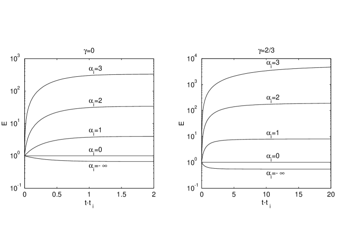
FIG. 1.: Evolution of the asymmetry parameter $E=Y(t)/X(t)$ (according to eqns. (7) and (8)) for several values of $\alpha_{i}=\log_{10}(D_{i})$ assuming $\gamma=0$ (left panel) and $\gamma=2/3$ (right panel) respectively. Note that time is given in units of $H^{-1}(t_{i})$.

What about the evolution of the domain walls? Based on rather general grounds, we expect it to have a number of similarities with the much better studied case of cosmic strings [6]. In particular, one can define a ‘characteristic length-scale’, which we shall denote by $L$, that can be roughly interpreted as a typical curvature radius or a correlation length of the wall network. It is also a length-scale that measures the total energy of the domain wall network per unit volume, since we can define

$$\rho\equiv\frac{\sigma}{L}\,,$$ (16)

where $\sigma$ is the domain wall energy per unit area. Note that in a more rigorous treatment that allowed for the expected build-up of small-scale ‘wiggles’ on the walls (in analogy with what happens for the case of cosmic strings [13]) each of these three length scales would be different. However, for our present purposes it is adequate to suppose that they are all similar.

Then we can expect to find two different evolution regimes. While the network is non-relativistic, we expect it to be conformally stretched by the cosmological expansion, and hence

$$L\propto a\,,\qquad\rho_{w}\propto a^{-1}\,.$$ (17)

In this case there is essentially no dynamics. An extreme example of this regime happens during inflation We can see from eqn. (5) that due to the very rapid expansion which occurs in the inflationary regime the time derivatives of the field $\phi$ rapidly approach zero so that the network of domain walls will simply be frozen in comoving coordinates.

On the other hand, once the network becomes relativistic, one expects it to evolve in a linear scaling regime where

$$L\propto t\,,\qquad\rho_{w}\propto t^{-1}\,.$$ (18)

This is the case of ‘maximal’ dynamics, in the sense that the network is evolving (in particular, losing energy by wall collisions and re-connections) as fast as allowed by causality. We note that previous work of Press, Ryder and Spergel [17] suggests that there may be logarithmic corrections to this linear regime.

III Numerical simulations

At late times (after the inflationary epoch) the universe is homogeneous and isotropic with $A=B=C$ with the average dynamics of the universe being specified by the evolution of the scale-factor $a(t)$. We now consider the evolution of isotropic and anisotropic defect networks in this background. In particular, we are interested in determining how the networks evolve as they re-enter the horizon, since if one finds differences in the dynamics of the two cases then this should translate into observational tests that will allow us to discriminate between then and hence probe pre-inflationary physics.

It is useful for numerical purposes to re-write equation (5) as a function of the conformal time $\eta$ defined by $d\eta=dt/a$. In this case equation (5) becomes

$${{\partial^{2}\phi}\over{\partial\eta^{2}}}+2\frac{\dot{a}}{a}{{\partial\phi}\over{\partial\eta}}-{\nabla}^{2}\phi=-a^{2}{{\partial V}\over{\partial\phi}}.$$ (19)

with

$${\nabla}^{2}={{\partial^{2}}\over{\partial x^{2}}}+{{\partial^{2}}\over{\partial y^{2}}}+{{\partial^{2}}\over{\partial z^{2}}}.$$ (20)

When making numerical simulations of the evolution of domain wall networks (or indeed other defects) it is also often convenient to modify the equation of motion for the scalar field $\phi$ in such a way that the comoving thickness of the walls is fixed in comoving coordinates. This is known as the PRS algorithm [17], and it is generally believed not to significantly affect the large-scale dynamics of domain walls.

We note, however, that recent high-resolution simulations [19] have revealed that the accuracy of this algorithm is not as good as has been claimed. This effect is expected to increase with increasing dynamic range. In particular, the PRS algorithm artificially prevents the build-up of small-scale features on the domain walls (or, for that matter, any other defect). This turns out to be crucial for a quantitatively accurate description of their evolution, and hence for a reliable analysis of their observational consequences. For our purposes in the present work, however, the PRS algorithm is enough as an approximation to the true wall dynamics. In a subsequent, more detailed publication we shall compare results obtained using this algorithm with those from the true wall dynamics.

Having clarified this point, we will modify the evolution equation for the scalar field $\phi$ in the isotropic phase according to the PRS prescription:

$${{\partial^{2}\phi}\over{\partial\eta^{2}}}+\beta_{1}\frac{\dot{a}}{a}{{\partial\phi}\over{\partial\eta}}-{\nabla}^{2}\phi=-a^{\beta_{2}}{{\partial V}\over{\partial\phi}}.$$ (21)

where $\beta_{1}$ and $\beta_{2}$ are constants. We choose $\beta_{2}=0$ in order for the walls to have constant comoving thickness and $\beta_{1}=3$ by requiring that the momentum conservation law for how a wall slows down in an expanding universe is maintained [17].

We perform two-dimensional simulations of domain wall evolution for which $\partial^{2}\phi/\partial z^{2}=0$. These have the advantage of allowing a larger dynamic range and better resolution than tree-dimensional simulations.

We solve equation (21) numerically assuming a matter-dominated Einstein-de-Sitter cosmology with $a\propto\eta^{2}$. We used a standard difference scheme second-order accurate in space and time and periodic boundary conditions (see [17] for a more detailed description of the algorithm and other related numerical issues).

The initial properties of the network of domain walls depend strongly on the details of the phase transition which originated them. It is conceivable that the initial network is already formed asymmetric with the walls being elongated along preferred directions. However, this is beyond the scope of the present paper. For our present purposes, we can ignore this possibility and assume that the initial domain wall network is statistically isotropic. This assumption will not modify the conclusions of the paper—if anything, any ab initio anisotropies would only enhance the effects we are describing.

Hence, we assume the initial value of $\phi$ to be a random variable between $-\phi_{0}$ and $\phi_{0}$ and the initial value of ${\dot{\phi}}$ to be equal to zero everywhere. We normalise the numerical simulations so that $\phi_{0}=1$. We set the conformal time at the start of the simulation and the comoving spacing between the mesh points to be respectively $\eta_{i}=1$ and $\Delta x=1$.

The wall thickness, defined by

$${\omega}_{0}={{\pi\phi_{0}}\over{\sqrt{2V_{0}}}}$$ (22)

is set to be equal to $5$. The kinetic energy of the field $\phi$ is calculated by

$$E_{kin}=\frac{1}{8\pi}\sum_{i,j}{\dot{\phi}}_{i,j}\,.$$ (23)

On the other hand, the rest energy of the walls is calculated by multiplying the comoving area of the walls, A, by the energy density per comoving area, which can be written as

$$\sigma=\frac{2\gamma_{w}V_{0}\omega_{0}}{3\pi^{2}}.$$ (24)

with $\gamma_{w}=(1-v_{w}^{2})^{-1/2}$, and $v_{w}$ is the value of the physical velocity of the domain walls. Finally the total area of the walls is defined as the area of the surfaces on which $\phi=0$ and is computed using the method described in ref. [17].

IV Results and discussion

As pointed out above, it will be of fundamental importance to study the dynamics of the wall network at late times, as the Hubble length becomes larger than the typical size of the major axis of a domain wall. A crucial issue will be the timescale required for the wall network to switch from the non-relativistic regime to the relativistic one. For our present purposes, the main difference between these two regimes is that a friction-dominated network can remain anisotropic if it froze out that way, whereas a relativistic network will rapidly become isotropic and erase any imprints from the earlier anisotropic phase. In our simulations we ignore the possibility that the network can be friction dominated due to particle scattering [13] when the domain walls come back inside the horizon—again, this would only enhance the effects we are describing.

FIG. 2.: The same physical size of the same domain wall simulation. The bottom one however has been stretched along the y direction by a factor of 2. The horizon size of the top box is 1/8 of the linear size of the box shown, and this is itself only a fraction 1/16 of the side of the whole simulation box.]

We consider three simulations with different initial conditions. In the first one (case I) we evolve the initial network generated in the manner specified in the previous section from the conformal time $\eta_{i}=1$. In the second one (case II) the initial conditions at the time $\eta_{i}=1$ were specified by the network configuration of the previous simulation at the conformal time $\eta_{*}=20$, with the velocities reset to zero. Physically, this corresponds to starting with the network outside the horizon. Finally, the case III is similar to the second one but with the initial network of case II stretched in the $y$ direction by a factor of $E=2$ (see fig. 2), and corresponds to the anisotropic case. We have performed $1024^{2}$ simulations for each of the three cases, plus an additional $2048^{2}$ run of case I, in order to test for possible box effects.

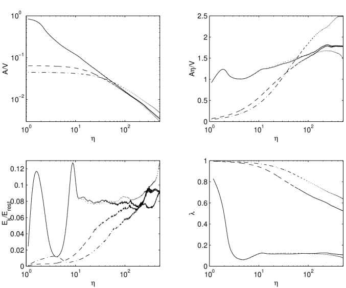
FIG. 3.: Evolution of several properties of a domain wall network as a function of the conformal time $\eta$ during the matter era. Here, $E_{k}$ and $E_{rest}$ are the kinetic and rest energies associated with the scalar filed $\phi$, $A/V$ is the comoving wall area per unit comoving volume of the two-dimensional simulations, $\lambda$ is a ‘scaling coefficient’ defined by $\lambda=d\ln(A\eta/V)/d\ln\eta$ and $\eta$ is the conformal time. The solid, dashed and dash-dotted curves correspond to $1024^{2}$ simulations with different initial conditions. Cases I and II have isotropic initial conditions but in case two the size of the domain walls becomes comparable with horizon only at a conformal time $\eta_{*}=20$. Case III is similar to case II but with the initial network of case II stretched in the $y$ direction by a factor of $E=2$ (see text). The dotted curve corresponds to a $2048^{2}$ run of case I.

For each run we plot (see fig. 3) the ratios $A/V$ and $A\eta/V$ (note that $A$ and $V$ are the comoving area and volume, respectively), as well as the ratio of the kinetic and rest energies, as in Press, Ryden and Spergel [17]. These are plotted from the beginning of the simulation until the time when the horizon becomes one half (for the $1024^{2}$ runs) or one quarter (for the $2048^{2}$ run) of the box size. In addition to these (which we plot mainly for the purposes of comparison with previous work [17]) we plot a ‘scaling coefficient’ which will be our main analysis tool. We will define it by analogy with the cosmic string case [11, 13], as follows. Assume that

$$\eta\frac{A}{V}\propto\eta^{\lambda}\,;$$ (25)

then what we plot is the ‘instantaneous’ or ‘effective’ value of $\lambda$ as a function of conformal time. For a given $\lambda$, the physical network correlation $L$ length will be evolving as

$$L\propto t^{1-\lambda/3}\,,\qquad\frac{L}{a}\propto\eta^{1-\lambda}\,.$$ (26)

Note that $\lambda$ can, in general, be a time-dependent quantity. However, for the two scaling regimes discussed above, we expect it to be a constant, namely

$$\lambda_{nr}=1\,$$ (27)

in the non-relativistic limit where the network is being conformally stretched, and

$$\lambda_{r}=0\,$$ (28)

in the linear scaling regime.

From these it is trivial to deduce the behaviour of $A/V$ and $A\eta/V$ in both scaling regime. One expects

$$\eta\frac{A}{V}\propto\eta\,\qquad\frac{A}{V}\propto const.$$ (29)

in the non-relativistc regime and

$$\eta\frac{A}{V}\propto const\,\qquad\frac{A}{V}\propto\eta^{-1}$$ (30)

in the linear scaling regime. Similarly, the ratio $E_{k}/E_{rest}$ should be a constant in the linear scaling regime (with its numerical value providing a measure of the characteristic network scaling speed), and it should approach zero in the non-relativistic limit.

Firstly, we note that the two case I runs produce very similar results: significant differences can only be seen at late times. This is an indication that the resolution we are using is adequate for our present purposes. As expected, the network in case I becomes relativistic very quickly, while those of cases II and III start in the extreme non-relativistic regime and only evolve away from it fairly slowly, after they re-enter the horizon.

More importantly, there are two non-trivial observations to be made. Firstly, we confirm that there is a correction to the linear scaling regime. We find

$$\lambda_{sc}\sim 0.12\,,$$ (31)

which corresponds to to evolve in a linear scaling regime where

$$L\propto t^{0.96}\,,\qquad\rho_{w}\propto t^{-0.96}\,,$$ (32)

in agreement with the previous result by Press, Ryden and Spergel [17]. This means that the network is not straightening out as fast as allowed by causality. Secondly, the rates at which the networks in cases II and III approach the relativistic regime are different. One might expect this on physical grounds: if the network is stretched in one direction, then there are in fact different ‘network correlation lengths’ for each direction, and interactions between the domain walls will tend to occur faster along the directions with smaller correlation lengths, and more slowly in the others.

Another way of saying this is that the network will only start evolving towards the relativistic regime when its larger axis has re-entered the horizon. Note that this mechanism also tends to make the domain wall network more isotropic. So one can naively say that the approach to the linear scaling regime takes longer in an anisotropic universe because the dynamics of the walls must accomplish two tasks (make the wall network relativistic and isotropic) rather than just one.

V Conclusion

In this paper we have discussed a simple example of what we believe to be a rather generic feature of topological defect models, namely that they can easily retain information about the properties of the very early universe. This information is encoded in the scaling (ie, ‘macroscopic’) and statistical (ie, ‘microscopic’) properties of the defect networks. This is even more relevant given the fact that defects can survive significant amounts of inflation. Hence, they can provide a unique probe of the pre-inflationary universe. The two crucial scales in the problem are the defect mass scale and the epoch when the defects come back inside the horizon.

Specifically, we have discussed the role of domain walls. We have highlighted the existence of two scaling regimes for the domain wall network, in agreement with previous work [17]. Furthermore, we have shown that an anisotropic network re-entering the horizon will take longer to approach scaling than an isotropic one. Hence, if the very early universe had an anisotropic phase which was erased by an inflationary epoch, and if domain walls are present, then the walls can retain an imprint of the earlier phase, and this can have important observational consequences, eg for structure formation scenarios.

As is well known, there are quite strong constraints [16, 6] on the mass of domain walls formed after inflation. These are basically due to the fact that their density will decay more slowly than the radiation and matter densities. However, essentially all of these can be evaded (or at least significantly relaxed) by walls forming before or during inflation (and also by walls evolving in a friction-dominated regime). Having said this, how could these anisotropies be detected? The most naive answer would be through their imprint on CMB, but this is only true if their energy density is not too low, and such models are constrained in a variety of other ways (not only from the cosmology side, but also from the high-energy physics side). The case of ‘light’ walls is therefore more interesting: note that just like in the case of ‘light strings’ [13], these are expected to be friction-dominated throughout most of the cosmic history. Here the observational detection of the effects we have described becomes somewhat non-trivial. The best way of doing it should be through observations of numbers of objects as a function of redshift in different directions (assuming that one has a reliable understanding of other possible evolutionary effects). Two specific examples would be large-scale velocity flows [20] and gravitational lensing statistics of extragalactic surveys [21].

Finally, there is also an important implication of our work if at least one of the minima of the scalar field potential has a non-zero energy density, which is an anisotropic non-zero vacuum density. In a subsequent, more detailed publication, we shall discuss this scenario in more detail, as well as the analogous one for cosmic strings.

To conclude, we have shown that the importance of topological defects as a probe of cosmological physics goes well beyond structure formation. Even if defects turn out to be unimportant for structure formation they can still (if detected) provide us with extremely valuable information about the physical conditions of the very early universe.

- [1] E.W. Kolb & M.S. Turner, The Early Universe, (Addison-Wesley, 1994).
- [2] A.H. Guth, Phys. Rev. D23, 347 (1981).
- [3] A.D. Linde, Particle Physics and Inflationary Cosmology (Harwood, Chur, Switzerland, 1990).
- [4] A.R. Liddle & D.H. Lyth, Phys. Rep. 231, 1 (1993); D.H. Lyth & A. Riotto Phys. Rep. 314, 1 (1999).
- [5] S. Gratton, T. Hertog & N.G. Turok, astro-ph/9907212 (1999).
- [6] A. Vilenkin & E. P. S. Shellard, Cosmic Strings and other Topological Defects, (Cambridge University Press: Cambridge, 1994).
- [7] Q. Shafi & A. Vilenkin, Phys. Rev. Lett. 52, 691 (1984); Q. Shafi & A. Vilenkin, Phys. Rev. D29, 1870 (1984).
- [8] J. Yokoyama, Phys. Lett. B212, 273 (1988); J. Yokoyama, Phys. Rev. Let. 63, 712 (1989).
- [9] H.M. Hodges & J.R. Primack, Phys. Rev. D43, 3155 (1991).
- [10] P.P. Avelino, R.R. Caldwell & C.J.A.P. Martins, Phys. Rev. D59, 123509 (1999).
- [11] C.J.A.P. Martins & E.P.S. Shellard, Phys. Rev. D53, 575 (1996); C.J.A.P. Martins & E.P.S. Shellard, Phys. Rev. D54, 2535 (1996).
- [12] P.P. Avelino, R.R. Caldwell & C.J.A.P. Martins, Phys. Rev. D56, 4568 (1997).
- [13] C.J.A.P. Martins, Quantitative String Evolution, Ph.D. Thesis, University of Cambridge (1997).
- [14] M. Bucher, A.S. Goldhaber & N.G. Turok, Phys. Rev. D52, 3314 (1995).
- [15] A. Vilenkin, Phys. Rev. D56, 3258 (1997).
- [16] Ya.B. Zel’dovich, I. Kobzarev & L.B. Okun, Soviet Phys. JETP, 40, 1 (1975).
- [17] W.H. Press, B.S. Ryden & D.N. Spergel, Ap. J. 347, 590 (1994).
- [18] M. Carmeli, Ch. Charach & S. Malin, Phys. Rep. 76, 79 (1981); J. Wainwright & G.F.R. Ellis, Dynamical Systems in Cosmology (Cambridge University Press, 1997).
- [19] E.P. Shellard, private communication (1999).
- [20] I. Zehavi & A. Dekel, astro-ph/9904221 (1999).
- [21] R. Quast & P. Helbig, Astron. Astroph. 344, 721 (1999).