COSMIC VELOCITIES 2000: A REVIEW
To Appear in Proceedings of the XXXVth Rencontres de Moriond:
Energy Densities in the Universe

I review the status of cosmic velocity analysis as of January 2000, with an emphasis on two key questions: (1) What is the scale of the largest bulk flows in the universe? and (2) What is the value of $\beta\equiv\Omega_{m}^{0.6}/b$ indicated by cosmic velocities, and what does this tell us about $\Omega_{m}$ itself? These are the most important issues for cosmic flow analysis, and each has been controversial in recent years. I argue that a preponderance of the evidence at present argues against very large scale ($\lower 1.72221pt\hbox{$\buildrel>\over{\sim}\,$}100\,h^{-1}\,{\rm Mpc}$) bulk flows, and favors $\beta\simeq 0.4$–$0.5,$ corresponding to a low-density ($\Omega_{m}\simeq 0.2$–$0.3$) universe.

1 Background

The study of cosmic flows emerged as a distinct subfield of cosmology in the late 1970s, spurred by the discovery of the Tully-Fisher (TF) and Faber-Jackson relations for spiral and elliptical galaxies, respectively. With these empirical correlations between galaxy luminosity and internal velocity as distance indicators, one could measure redshift-independent distances for galaxies out to tens or even hundreds of megaparsecs. Both the TF relation and the successors of Faber-Jackson—the $D_{n}$-$\sigma$ and Fundamental Plane (FP) relations—yield distances with $\sim 15$–$20\%$ accuracy. Although hopes for further improving the accuracy of TF and FP have proved unfounded, these distance indicators have remained the workhorses of cosmic velocity analysis for two decades. Only in recent years have newer and more accurate distance indicator methods—in particular Type Ia Supernovae and Surface Brightness Fluctuations—begun to complement (not supplant) TF and FP, as discussed further below.

The early scientific emphasis in flow studies was on determining the amplitude of Virgo infall (e.g., Tonry & Davis 1981; Aaronson et al. 1982). The Virgo cluster and its environs were then thought to dominate the local flow field. It has since been recognized that the local velocity field is more complex. There are a number of nearby attractors and voids, as well as the tidal effect of distant mass concentrations. The most sophisticated models of the local velocity field now use gravitational instability theory to predict peculiar velocities on the basis of the galaxy density field observed in redshift surveys. The redshift survey most widely used for this purpose is the IRAS redshift survey, both in its older, 1.2 Jy (Fisher et al. 1995) and newer PSCz (Saunders et al. 2000) incarnations. If one assumes IRAS galaxies trace mass and adopts the approximations of linear theory, comparison of predicted velocities with the observed ones constrains the parameter $\beta_{I}=\Omega_{m}^{0.6}/b_{I}.$ Here, $b_{I}$ is the biasing parameter for IRAS galaxies, a measure of whether IRAS galaxies are more ($b_{I}>1$) or less ($b_{I}<1$) clustered than mass. (The subscript is needed because different redshift samples have different clustering amplitudes, and thus different biasing parameters.)

Measurement of $\beta_{I}$ has thus become one of the main thrusts of cosmic flow analysis in the 1990s. Early in the decade, when there was a widespread theoretical prejudice in favor of an $\Omega_{m}=1$ universe, it was thought peculiar velocities might be the key to proving it. On large scales, the argument went, galaxies should trace the dominant dark matter, and the large-scale peculiar field should therefore reflect the underlying Einstein-de Sitter nature of the universe. The earliest efforts in this direction indeed seemed to bear out this suspicion, finding $\beta_{I}\approx 1.3,$ suggestive of $\Omega_{m}=1$ (Dekel et al. 1993). More recently, however, cosmic flow-based estimates of $\beta_{I}$ have often, though not invariably, produced values in the $0.4$–$0.6$ range, consistent with a low-density cosmology. In §3 I will summarize recent work done on this problem, and explain why I believe the low $\beta_{I}$ values are more likely to be correct.

Another aim of cosmic flow studies first arose serendipitously: efforts to detect bulk flow on very large ($\lower 2.15277pt\hbox{$\buildrel>\over{\sim}\,$}100h^{-1}\,{\rm Mpc}$) scales. This work was propelled by the discovery, in 1987, of a bulk flow stretching across the sky by the “7-Samurai” (7S) group (Dressler et al. 1987). Working with the newly discovered $D_{n}$-$\sigma$ relation, the 7S found that elliptical galaxies out to $\sim 3000\,\,{\rm km}\,{\rm s}^{-1}$ redshift exhibited fairly uniform Hubble expansion from the vantage point of the Local Group (LG) barycenter. But the LG is known to move at $630\,\,{\rm km}\,{\rm s}^{-1}$ with respect to the Cosmic Microwave Background radiation (CMB), as indicated by the CMB dipole anisotropy. Thus, the implication of the 7S findings was that the ellipticals were streaming at $\sim 600\,\,{\rm km}\,{\rm s}^{-1}$ relative to the CMB. If there is any validity to Big Bang cosmology, though, the CMB defines an absolute standard of rest—the “cosmic rest frame,” as it were. The 7S finding thus inaugurated a long-standing puzzle in cosmology: how can large-scale, coherent bulk flows exist in a universe that seems to be so uniform on large scales?

The puzzle deepened in the following decade, with a number of groups confirming a 7S-like bulk flow, and, in several cases, finding that it continued to scales three or four times the 7S volume. The current controversy may be framed as “what is the scale of the largest bulk flow,” or, equivalently, as one of convergence scale: at what distance are the galaxies within a spherical shell finally at rest in the CMB frame? Some astronomers (this author included) have been led to wonder whether such a convergence scale existed; perhaps the CMB-defined “cosmic rest frame” was offset by $600\,\,{\rm km}\,{\rm s}^{-1}$ from the frame in which uniform Hubble expansion is observed—a conjecture which, if correct, would call into question some of the fundamental tenets of cosmology. Fortunately—at least if you like agreement between theory and observation—it now appears that the convergence to the CMB has been detected at a distance of $\sim 50$–$60h^{-1}\,{\rm Mpc}.$ Or at least, that is what I will argue in §2, when I summarize results from newly completed surveys.

2 The Scale of the Largest Bulk Flows

First we should ask, from the perspective of cosmology, Why are bulk flows interesting? In particular, what does their convergence scale tell us?

The answer lies in the sensitivity of bulk flows to long-wavelength modes of the mass fluctuation power spectrum. Mass conservation in the linear regime of gravitational instability tells us that

$$\nabla\cdot\mathbf{v}=-\Omega_{m}^{0.6}\delta,$$ (1)

where $\mathbf{v}$ is the peculiar velocity vector and $\delta$ is the mass density contrast. The corresponding equation in Fourier space is $\mathbf{k}\cdot\mathbf{v}_{k}=-\Omega_{m}^{0.6}\delta_{k},$ where the subscript denotes Fourier transform. Thus, $|\mathbf{v}_{k}|\propto\delta_{k}/k,$ which is to say, long-wavelength perturbations (small $k$) have a larger impact on large-scale peculiar velocities than they do on mass fluctuations.

One can flesh out these ideas by calculating the mean square bulk velocity on a scale $R:$

$$\left\langle v^{2}(R)\right\rangle=\frac{\Omega_{m}^{1.2}}{2\pi^{2}}\int_{0}^{\infty}P(k)\,\widetilde{W}^{2}(kR)\,dk\,,$$ (2)

where $P(k)$ is the mass fluctuation power spectrum and $\widetilde{W}^{2}(kR)$ is the Fourier transform of a top-hat window of radius $R.$ In Figure 1 the rms expected bulk velocity, $V_{rms}(R)=\sqrt{\left\langle v^{2}(R)\right\rangle},$ is plotted against $R$ (left panel) and $\Omega_{m}$ (right panel) for COBE-normalized CDM power spectra. The left panel assumes a canonical $\Omega_{m}=0.3,$ $\Omega_{\Lambda}=0.7$ universe. For comparison, the rms density fluctuation $\sigma_{{}_{M}}(R)=\left\langle(\delta M)/M)^{2}(R)\right\rangle$ is also plotted. Note that $\sigma_{{}_{M}}$ drops much more rapidly with scale than does $V_{rms}.$ This is a result of the sensitivity of large-scale bulk flow to long-wavelength modes of the power spectrum. An observational consequence is that while redshift surveys have difficulty probing the power spectrum on scales $\lower 2.15277pt\hbox{$\buildrel>\over{\sim}\,$}100h^{-1}\,{\rm Mpc},$ bulk flow studies can in principle do so.

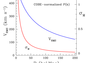
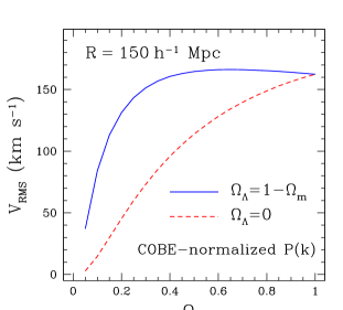
Figure 1: Left panel: Expected rms bulk velocity of a sphere of radius $R,$ for an $\Omega_{m}=0.3,$ $\Omega_{\Lambda}=0.7$ universe. Also shown is the mass density fluctuation $\sigma_{{}_{M}}(R).$ Right panel: rms bulk velocity of an $R=150h^{-1}\,{\rm Mpc}$ sphere versus $\Omega_{m}$ for open and flat universes.

Closer inspection of the left panel also shows why large-amplitude ($V\lower 2.15277pt\hbox{$\buildrel>\over{\sim}\,$}500\,\,{\rm km}\,{\rm s}^{-1}$), large-scale $R\lower 2.15277pt\hbox{$\buildrel>\over{\sim}\,$}60h^{-1}\,{\rm Mpc}$ are potentially problematic for standard structure-formation scenarios. In the CDM-type models shown here, there simply isn’t enough large-scale power to drive such flows. Stated another way, the CDM universe approaches homogeneity sufficiently rapidly with increasing scale that the coherence scale of bulk flows should be a few tens of megaparsecs at most. Moreover, the right panel shows, perhaps counterintuitively, that boosting the matter density doesn’t help. (This is a consequence of imposing COBE-normalization; normalizing the power spectrum to the cluster abundance does not substantially change our conclusions.)

However, high-amplitude bulk motions on scales $\lower 2.15277pt\hbox{$\buildrel>\over{\sim}\,$}100h^{-1}\,{\rm Mpc}$ are just what were found by three surveys conducted in the early and mid 1990s. The first of these, and the one which has achieved the greatest notoriety, was the Brightest Cluster Galaxy (BCG) survey by Lauer & Postman (1994; LP). LP used the BCGs as standard candles, thus obtaining distances to over 100 Abell clusters out to $15,000\,\,{\rm km}\,{\rm s}^{-1}$ redshift, and found them to be coherently moving relative to the CMB at $\sim 700\,\,{\rm km}\,{\rm s}^{-1}.$ The combination of large scale and high amplitude places the LP result far above the expected $V_{rms}$ values in Figure 1.

More recently, two large surveys of cluster galaxies appeared to confirm the scale and amplitude (but not the direction) of the LP result. The Streaming Motions of Abell Clusters (SMAC) survey of Hudson et al. (1999) used the FP relation to measure cluster ellipticals to about the same depth as the LP survey, and found a $600\,\,{\rm km}\,{\rm s}^{-1}$ flow, in roughly the same direction as the that found by 7S a decade earlier. And in a Tully-Fisher survey of cluster galaxies in a shell between $\sim 9000$ and $13,000\,\,{\rm km}\,{\rm s}^{-1},$ I (Willick 1999, LP10K) found a streaming motion of about $700\,\,{\rm km}\,{\rm s}^{-1}$ in roughly the same direction as SMAC. The above results are summarized in Table I, along with another bulk flow measurement based on more nearby galaxies from the Mark III Catalog of TF and $D_{n}$-$\sigma$ data (Willick et al. 1997), as measured by the POTENT algorithm (on which more in § 3).

Table I. Recent Bulk Flow Measurements

Survey	$R$ ($\,{\rm km}\,{\rm s}^{-1}$)	$V_{B}$ ($\,{\rm km}\,{\rm s}^{-1}$)	Comments
Lauer-Postman (LP)	15000	700	BCG
Willick (LP10K)	12000	700	TF
Hudson et al. (SMAC)	14000	600	FP
Dekel et al. (POTENT)	6000	350	TF+$D_{n}$-$\sigma$

The four results above argue for large bulk flows, but are not fully consistent. The SMAC, LP10K, and POTENT/Mark III flows agree in direction, but the LP flow is nearly orthogonal. Also, the smaller amplitude of the smaller scale POTENT/Mark III measurement is puzzling; one would expect bulk flow amplitude to diminish monotonicaly with scale (Figure 1). Even without evidence to the contrary, then, the above results are less than convincing.

More importantly, however, 1999 saw the announcements of new survey results that contradict the findings of Table 1. The nearby Type Ia Supernova (SN Ia) data have accumulated, and as reported by Riess (2000), the sample of SN Ia distances within $\sim 10,000\,\,{\rm km}\,{\rm s}^{-1}$ redshift show no evidence for bulk flow. This is quite important, because the SN Ia data are of a fundamentally different nature than the other distance indicators employed in cosmic flow studies. Also, as shown in the cosmological context, SN Ia have small scatter, $\sim 0.15$ mag. The EFAR FP survey of Colless et al. (2000) similarly finds no bulk motion on a large scale, and in particular is inconsistent with LP at better than 99% confidence. Similar results have been obtained by Dale, Giovanelli, and coworkers from their extensive TF surveys (as summarized by Dale & Giovanelli 2000). The key findings of these surveys, plus that of the Shellflow survey, to which I turn next, are summarized in Table 2.

Table II. More Recent Bulk Flow Measurements

Survey	$R$ ($\,{\rm km}\,{\rm s}^{-1}$)	$V_{B}$ ($\,{\rm km}\,{\rm s}^{-1}$)	Comments
Riess et al.	$10000$	$\approx 0$	SN Ia
Courteau et al. (SHELLFLOW)	$6000$	$\approx 0$	TF
Colless et al. (EFAR)	$\sim 10000$	$\approx 0$	FP
Dale & Giovanelli (SFI)	$6000$	$\approx 0$	TF
Dale & Giovanelli (SCI/SCII)	$\sim 15000$	$\approx 0$	TF

A group of us who were active in cosmic velocity measurement and analysis (M. Strauss, S. Courteau, M. Postman, D. Schlegel, and myself) realized in 1995 that a critical issue had not been properly addressed in the then-extant Tully-Fisher surveys: the need for extremely uniform data across the sky. We proposed for and were granted extensive NOAO time for the Shellflow project, a TF survey of a shell of 300 galaxies between $5000$ and $7000\,\,{\rm km}\,{\rm s}^{-1}$ redshift. By using identical observational setups from northern and southern hemisphere NOAO telescopes we ensured that data nonuniformity could not produce spurious peculiar velocities.

In a recent paper (Courteau et al. 2000) we reported our main result: the bulk flow of the shell centered at $6000\,\,{\rm km}\,{\rm s}^{-1}$ is $70^{+100}_{-70}\,\,{\rm km}\,{\rm s}^{-1},$ i.e., is consistent with being at rest in the CMB frame. The residuals with respect to a fit that assumes pure Hubble flow in the CMB frame are shown in Figure 2. The points are everywhere consistent with being due to TF scatter, not coherent peculiar velocities. Inflowing and outflowing points are well mixed at all positions, indicating the absence of coherent motions.

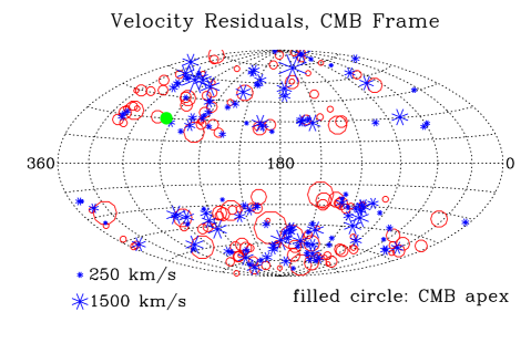
Figure 2: Apparent peculiar velocity residuals (TF residuals converted into velocities) of Shellflow galaxies for a pure Hubble flow fit. Point size is proportional to the velocity amplitude, with fiducial values indicated at the lower left. Circles and asterisks represent inflowing and outflowing objects, respectively.

Having worked with the Shellflow data myself, I am confident that it is of very good quality, and am convinced that systematic errors have a very small effect, if any on our results. I therefore find the conclusion of insignificant bulk flow highly persuasive. The Shellflow results refer to a specific scale, namely, a $60h^{-1}\,{\rm Mpc}$ sphere. They do not directly test the LP, SMAC, and LP10K results of Table 1. However, because abundant evidence indicates that the universe approaches homogeneity monotonically with increasing scale size, I believe that the Shellflow result, if correct, is physically inconsistent with the LP, SMAC, and LP10K findings, and that the latter are therefore not to be taken at face value.

One should not, however, judge the LP, SMAC, and LP10K authors harshly (and I have an obvious reason for hoping you don’t!). Measuring distortions of the Hubble expansion that are at the level of a few percent is a challenging task, given the limitations of the distance indicator techniques we work with. False detections, if that is what they are, will most likely be seen in hindsight as inevitable products of initial efforts at a very difficult measurement.

3 The Value of $\beta_{I}$

In considering the scientific implications of large-scale bulk flow surveys, I made no mention of comparison with redshift surveys. That is because the full-sky redshift surveys we have are not reliable enough, at distances $\lower 2.15277pt\hbox{$\buildrel>\over{\sim}\,$}150h^{-1}\,{\rm Mpc},$ to predict what the bulk flows should be on such scales. The situation changes when we talk about the velocity field within $\sim 50h^{-1}\,{\rm Mpc}.$ At these distances both the peculiar velocity and galaxy density fields are mapped with enough accuracy to do a detailed comparsion. The goals of this comparison are (1) to verify that the two maps are compatible with the gravitational instability paradigm, and (2) assuming they are, to measure $\beta_{I}=\Omega_{m}^{0.6}/b_{I},$ and if possible to go further and measure $\Omega_{m}$ itself.

The theoretical bases of the comparison are either of two forms of the linear velocity-density relation. One is the differential form, Eq. (1), which for comparison of observables is written as

$$\nabla\cdot\mathbf{v}(\mathbf{r})=-\beta_{I}\delta_{I,g}(\mathbf{r})\,,$$ (3)

where $\delta_{I,g}(\mathbf{r})$ is the galaxy overdensity as determined by an IRAS redshift survey. The other is the corresponding integral form,

$$\mathbf{v}(\mathbf{r})=\frac{\beta_{I}}{4\pi}\int d^{3}\mathbf{r}^{\prime}\,\frac{\delta_{I,g}(\mathbf{r}^{\prime})(\mathbf{r}^{\prime}-\mathbf{r})}{\left|\mathbf{r}^{\prime}-\mathbf{r}\right|^{3}}\,.$$ (4)

In both Eqs. (3) and (4), the spatial positions $\mathbf{r}$ are assumed to be measured in velocity units—i.e., they are distances in units of the Hubble velocity. In this way, the Hubble constant itself is removed from the analysis, which is (needless to say) a useful simplification.

Although the two forms of the velocity-density relation are equivalent, they lead to two rather different analytical approaches to measuring $\beta_{I}.$ Because the controversy between the “high” and the “low” (see §1) values of $\beta_{I}$ appears to revolve around this distinction, it is worth taking a moment to understand it. To apply Eq. (3), one needs to map out the three-dimensional velocity field $\mathbf{v}(\mathbf{r}),$ differentiate it, and finally compare it to the galaxy density field to determine $\beta_{I}.$ Because only the radial component of $\mathbf{v}$ is observable, one first needs an ansatz for “three-dimensionalizing” the inherently one-dimensional velocity data. An elegant approach to this problem was developed by Bertschinger & Dekel (1989; see Dekel 1994 for a review), who argued that the large-scale velocity field should be irrotational and thus expressible as the gradient of a potential function, which could itself be computed by integrating the observed, radial velocities along rays. This algorithm, known as POTENT, thus produces a 3D velocity field, smoothed on a rather large (typically $12h^{-1}\,{\rm Mpc}$) scale, which can be differentiated and then used in Eq. (3).

Eq. (4) suggests a different approach. Rather than heavily processing the velocity data, one carries out the indicated integration using the redshift survey data. One thus obtains a predicted peculiar velocity field as a function of $\beta_{I},$ of which only the radial component, $u(\mathbf{r})=\mathbf{v}(\mathbf{r})\cdot\mathbf{r}/r,$ is used in the subsequent analysis. The predicted $u(\mathbf{r})$ is compared with the observed radial peculiar velocities from the TF (FP, etc.) data sets; the final estimate of $\beta_{I}$ is that which yields the closest match predictions and observations.

The two approaches to measuring $\beta_{I}$ are known as the density-density (d-d) and velocity-velocity (v-v) comparisons. It is notable that d-d comparisons, all done using POTENT to reconstruct the 3D velocity field, have consistently produced values of $\beta_{I}$ consistent with unity—and thus, to the extent $b_{I}$ is itself not so different from one, implicit estimates of $\Omega_{m}$ near unity as well. The 1993 paper by Dekel et al. was already mentioned (see §1). A more recent application of POTENT, using improved peculiar velocity data, was that of Sigad et al. (1998), who found $\beta_{I}=0.89\pm 0.1.$

Since about 1995, several v-v alternatives to the POTENT approach have been developed for measuring $\beta_{I}.$ They have differed in the way in which the IRAS (or other) redshift data are used to predict peculiar velocities, and in the way the predicted and observed peculiar velocities are compared. But as v-v methods they have more in common with one another than with POTENT; in particular, the heavy computational work is done with the redshift data, while the TF (FP, etc.) data are used only in a limited, statistical sense. These methods include the Least Action Principle approach of Shaya, Tully, & Peebles (1995), who obtain $\beta_{I}\approx 0.35\pm 0.1$), the VELMOD method of Willick et al. (1997) and Willick & Strauss (1998), who obtain $\beta_{I}=0.5\pm 0.05,$ and the ITF method (Davis, Nusser, & Willick 1996) which, applied to the Type Ia Supernova data produced a value of $\beta_{I}=0.4\pm 0.1.$

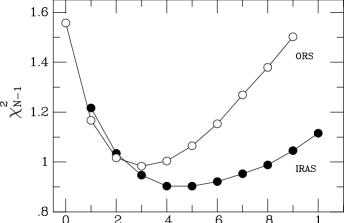
Figure 3: Left panel: VELMOD likelihood statistic ${\cal L}$ versus $\beta_{I},$ for the IRAS-predicted velocity field and the Mark III Catalog Tully-Fisher data. Adapted from Willick & Strauss (1998). Right panel: Reduced $\chi^{2}$ versus $\beta$ for the SBF velocity sample compared with IRAS and Optical Redshift Survey (ORS) predictions. The best fit for IRAS is $\beta_{I}=0.44\pm 0.08.$ Adapted from Blakeslee et al. (2000).

Figure 3 shows representative results from two v-v analyses. The left panel shows the VELMOD results from Willick & Strauss (1998). The statistic plotted is ${\cal L}=-2\ln P,$ where $P$ is the probability of observing the TF data given the IRAS velocity model. (The calculation is done for the “inverse” TF relation, which is immune to selection biases.) The minimum of the curve occurs at the maximum likelihood value of $\beta_{I},$ and its curvature yields the $1\,\sigma$ error, as indicated on the plot.

The right panel shows the first use of the new Surface Brightness Fluctuation (SBF) data set in $\beta$-measurement, as reported by Blakeslee et al. (2000). As was stated above in connection with SN Ia data, it is essential to carry out these experiments with independent distance indicators, and the SBF method is quite distinct from Tully-Fisher. Moreover, like SN Ia, SBF distances are on average about twice as accurate as TF distances, and have the additional advantage of having well-determined errors. In Figure 3, the SBF data are compared with velocities predicted by IRAS and the Optical Redshift Survey (ORS). The minimum $\chi^{2}$ is achieved for $\beta_{I}=0.44\pm 0.08,$ consistent with the VELMOD TF results. (The ORS galaxies are more clustered than IRAS galaxies, and therefore yield a lower $\beta$ value.)

A truly convincing explanation for this discrepancy between the v-v and d-d $\beta$ values has not yet been found. It seems to me, however, that the v-v comparison is a more robust procedure. In it, the intensive data manipulation is done on the redshift survey data, which is by its nature more reliable than the distance indicator data (redshifts errors are fractionally very small; redshift-independent distance errors are always $\sim 20\%$). In the d-d comparison, it is the data set with much larger scatter and non-Gaussian errors that is subjected to intensive manipulation. In particular, the d-d comparison requires that noisy data first be smoothed, then integrated, and then differentiated in three dimensions. There is ample opportunity in this procedure for errors to propagate. The same noisy data in the v-v studies are left virtually untouched, save for the statistical comparison with their predicted values. This procedure is far more stable. For this reason I consider the low $\beta$ values derived from the v-v analyses to be more reliable.

4 Summary

I have argued that the two major controversies in cosmic flow analysis have been largely resolved in the last few years. With regard to bulk flows, most recent surveys show convergence to the CMB frame by a distance of $\sim 60h^{-1}\,{\rm Mpc}.$ A corollary is that the observed bulk motions do not require more large-scale power than is provided by COBE-normalized CDM density fluctuation spectra. With regard to the value of $\beta_{I}=\Omega_{m}^{0.6}/b_{I},$ a number of independent analyses now suggest a low value, $\beta_{I}\simeq 0.4$–$0.5.$ If the IRAS galaxies are nearly unbiased with respect to mass, a reasonable if not airtight hypothesis, these $\beta$-values imply a density parameter $\Omega_{m}\simeq 0.2$–$0.3.$

A word of caution is in order, however. The above conclusions represent a consensus view, not a unanimous one. The bulk flow detections listed in the first three rows of Table 1 have not been in any sense “refuted,” which is to say as far as we know there is nothing wrong with the data. New surveys, such as FP200 (see http://astro.uwaterloo.ca/$\sim$mjhudson/fp200 for details) will, it is hoped, settle the issue definitively. Similarly, while a majority of recent velocity-density comparisons favor low $\beta_{I},$ the reason for the discrepant POTENT result, $\beta_{I}\approx 0.9,$ is not well understood. Tests of methods such as POTENT and VELMOD using N-body simulations are under way, and may clarify things. Moreover, the coming decade will bring much larger TF data sets from the DENIS and 2MASS infrared surveys. As always, these new data sets, if they live up to their promise, are our best hope for putting any remaining contoversy to rest.

References

- [1] Aaronson, M., Huchra, J., Mould, J., Schechter, P.L., & Tully, R.B. 1982, ApJ, 258, 64
- [2] Bertschinger, E., & Dekel, A. 1989, ApJ, 336, L5
- [3] Blakeslee, J.P., et al. 2000, in Cosmic Flows 1999: Towards an Understanding of Large-Scale Structure, eds. S. Courteau, M.A. Strauss, & J.A. Willick (ASP Conference Series)
- [4] Colless, M., et al. 2000, in Cosmic Flows 1999: Towards an Understanding of Large-Scale Structure, eds. S. Courteau, M.A. Strauss, & J.A. Willick (ASP Conference Series)
- [5] Courteau, S., Willick, J.A., Strauss, M.A., Schlegel, D., & Postman, M. 2000, astro-ph/0002420
- [6] Dale, D.A., & Giovanelli, R. 2000, in Cosmic Flows 1999: Towards an Understanding of Large-Scale Structure, eds. S. Courteau, M.A. Strauss, & J.A. Willick (ASP Conference Series)
- [7] Davis, M., Nusser, A., & Willick, J. A. 1996, ApJ, 473, 22
- [8] Dekel, A., Bertschinger, E., Yahil, A., Strauss, M., Davis, M., & Huchra, J. 1993, ApJ, 412, 1
- [9] Dekel, A. 1994, ARA&A, 32, 271
- [10] Dressler, A. et al. 1987, ApJ, 313, L37
- [11] Fisher, K.B., Huchra, J.P., Strauss, M.A., Davis, M., Yahil, A., & Schlegel, D. 1995, ApJS, 100, 69
- [12] Hudson, M.J., Smith, R.J., Lucey, J.R., Schlegel, D.J., & Davies, R.L. 1999, ApJ, 512, L79
- [13] Lauer, T. R., & Postman, M. 1994, ApJ, 425, 418
- [14] Riess, A.G., Davis, M., Baker, J., & Kirshner, R.P. 1997, ApJ, 488, L1
- [15] Riess, A.G. 2000, in Cosmic Flows 1999: Towards an Understanding of Large-Scale Structure, eds. S. Courteau, M.A. Strauss, & J.A. Willick (ASP Conference Series)
- [16] Saunders, W. et al. 2000, astro-ph/0001117
- [17] Sigad, Y., Eldar, A., Dekel, A., Strauss, M.A., & Yahil, A. 1998, ApJ, 495, 516
- [18] Tonry, J.L. & Davis, M. 1981, ApJ, 246, 680
- [19] Willick, J. A., et al. 1997, ApJS, 109, 333
- [20] Willick, J.A., Strauss, M.A., Dekel, A., & Kolatt, T. 1997, ApJ, 486, 629
- [21] Willick, J.A., & Strauss, M.A. 1998, ApJ, 507, 64
- [22] Willick, J.A. 1999, ApJ, 522, 647