Structure of the Large Magellanic Cloud from 2MASS

Abstract

We derive structural parameters and evidence for extended tidal debris from star count and preliminary standard candle analyses of the Large Magellanic Cloud based on Two Micron All Sky Survey (2MASS) data. The full-sky coverage and low extinction in $K_{s}$ presents an ideal sample for structural analysis of the LMC.

The star count surface densities and deprojected inclination for both young and older populations are consistent with previous work. We use the full areal coverage and large LMC diameter to Galactrocentric distance ratio to infer the same value for the disk inclination based on perspective.

A standard candle analysis based on a sample of carbon long-period variables (LPV) in a narrow color range, $1.6<J-K_{s}<1.7$ allows us to probe the three-dimensional structure of the LMC along the line of sight. The intrinsic brightness distribution of carbon LPVs in selected fields implies that $\sigma_{M}\hbox{ \hbox to0.0pt{\raise 1.82986pt\hbox{$<$}\hss}\lower 2.79857pt\hbox{$\sim$} }0.2^{m}$ for this color cut. The sample provides a direct determination of the LMC disk inclination: $42.3^{\circ}\pm 7.2^{\circ}$.

Distinct features in the photometric distribution suggest several distinct populations. We interpret this as the presence of an extended stellar component of the LMC, which may be as thick as $14$ kpc, and intervening tidal debris at roughly 15 kpc from the LMC.

1 Introduction

Morphologically, the LMC is an irregular barred spiral galaxy with three spiral arms and an extended outer loop of stellar material de Vaucouleurs & Freeman (1973). Based on deprojection and photometric distances (e.g. de Vaucouleurs 1957, 1980), its disk is inclined at an angle of $27^{\circ}$ to the plane of the sky. The disk exhibits solid body rotation out to $2.5^{\circ}$ with a rotation center at $5^{h}21^{m},-69^{\circ}17^{\prime}\,(1950)$, about $0.6^{\circ}$ north of the optical center of the bar. This kinematic signature is present in a variety of tracers: HI gas, planetary nebulae, HII regions, supergiants, CH stars, etc. Freeman et al. (1983) have examined kinematics of rich star clusters with ages between $100$ Myr and $10$ Gyr. They found that young clusters rotated with HI gas, while the older ones (SWB VII; Searle et al. 1980) formed a flattened rotating system with dispersion along the line of sight $\sigma\sim 18$ km/s. A later study of more extended sample of outer LMC clusters Schommer et al. (1992) confirmed the absence of isothermal pressure-supported spheroid. All this has led to the standard view that the LMC is a geometrically thin object.

However, recent studies have suggested that the LMC may have an extended component. First, the evidence for a flattened spheroid population was found in the kinematics of old long-period variables Hughes et al. (1991). Kunkel et al. (1997) describe a population of carbon stars out to 12 kpc from the LMC center. These authors interpret these in the context of a thin disk model and derive a rotation curve and mass estimate. However, Weinberg (2000) argues that the LMC should be evolving rapidly in the Milky Way tidal field, based on both analytic calculations and n-body simulations. The tidal field causes the LMC disk axis to precess and torques disk orbits out of the disk plane, causing a strongly flared, spheroidal-like distribution in the outer Cloud and loss of stars and gas. This interaction leads to an a spatially extended population while roughly preserving the disk-like kinematic signature (i.e., small $\sigma$).

The detection of, or strict limits on, the predicted extended distribution would resolve these views and is one of the goals for the present study. Our star count analysis is based on fitting the projected spatial density of several LMC populations among those identified in Nikolaev & Weinberg (2000; hereafter NW00) based on their location in the color-magnitude diagram (CMD) of the field. The late-type giant populations are dominated by the LMC and may be used as tracers of the spatial structure of the Cloud. Each population is fitted by two models: 1) thin exponential disk and 2) spherical power law model. Our best-fit models based on circular disks give the inclination of the LMC to the line of sight $i\approx 24^{\circ}-28^{\circ}$ and the position angle of the disk $\theta\approx 165^{\circ}-174^{\circ}$, in good agreement with previous estimates. The direction of the LMC disk inclination is also determined. In short, projected 2MASS star counts reproduce the standard LMC inferences.

The near-infrared 2MASS photometry easily discriminates carbon stars in the color-magnitude diagram. While the 2MASS single-epoch survey of the LMC does not provide variability information, we identified a region of the CMD populated nearly exclusively by carbon-rich AGB stars (Region J in NW00), which are also long-period variables (LPVs). This identification is reinforced by recent analyses of MACHO data Alves et al. (1998); Wood (1999), although roughly $25\%$ could be binaries Wood (1999). LPVs obey period-luminosity-color (PLC) relations (e.g., Feast et al. 1989), and based on the PLC relations, the LPVs in a narrow color range ($1.6<J-K_{S}<1.7$) are standard candles with $\sigma_{K}\approx 0.3^{m}$. Their photometric distribution in selected LMC fields has a least three distinct components: a well-defined narrow distribution due to LMC disk and two secondary peaks at fainter and brighter magnitudes. The differential photometric distance to the central disk peak provides a direct determination of the inclination: $42.3^{\circ}\pm 7.2^{\circ}$. This value is consistent with but larger than those inferred by deprojecting isopleths. The secondary peak could in principle be due to stellar blends, geometric structure, interstellar reddening, distribution of periods, gradient in age and metallicity, or contaminating population of overtone pulsators in the sample. We carefully examine the possible origins of this secondary component, and conclude that most likely explanation is spatial structure. This interpretation is bolstered by the good match of the central peak, which includes known fundamental mode pulsators, with the established LMC disk inclination. This implies the presence of an extended component of the LMC, which may be as thick as 14 kpc along the line of sight. This component is thicker than the 2.8 kpc flattened spheroid suggested by Hughes et al. (1991) from kinematic data and may be streams of material rather than be smooth and well-mixed. The bright peak is then an intervening population at a distance of roughly 35 kpc and the existence of relatively young carbon-rich AGB stars suggests tidal debris.

The outline for the paper follows. In the main section, we briefly describe the 2MASS sample (§2), and present the star count (§3) and the standard candle (§4) analyses of the LMC. In particular, §4.1 describes the selection of standard candles, §4.2 gives the details of the standard candle analysis and §4.3 presents the main results. The major conclusions are summarized in §5.

2 Observations

The LMC field, (4^h00^m to 6^h 56^m in right ascension, $-78^{\circ}$ to $-60^{\circ}$ in declination, J2000.0) has been observed by 2MASS and is included in the most recent data release. Details of the data reduction and sample selection are described in NW00. Figure 1 shows both the projected spatial distribution of sources and the color-magnitude diagram of the field.

Figure 1: Left panel: Density distribution of 2MASS sources in the LMC field. Contour levels are labeled in units of $10^{3}$ deg^-2. The arrow points in the direction of Galactic center. Right panel: CMD of the field showing 12 regions corresponding to major features of the diagram. Contour levels are logarithmic, from $2.0$ to $6.0$, spaced by $0.5$.

The color-magnitude diagram also shows the location of 12 regions analyzed in NW00. Total number of sources in our sample is 823,037.

NW00 examined the populations in selected CMD regions and associated the features with known populations of stars (cf. Table 2 of NW00). Here, we take an in-depth look at the spatial distribution of sources in seven of those regions (Table 1) which contain mostly LMC stars. These seven areas of the CMD account for a quarter of all sources in the field.

Table 1: Stellar populations of selected CMD regions.

Region	$N_{src}$	${f_{Gal}}^{\rm a}$	LMC populations
A	6,659	0.15	Young O,B,A supergiants, O3—O6 dwarfs
E	166,263	0.05	Low- and intermediate-mass RGB stars, E-AGB stars
F	22,134	0	Oxygen-rich AGB stars, E-AGB and TP-AGB, LPVs
G	1,438	0	Luminous E-AGB stars, O-rich LPVs
H	2,450	0.05	Red supergiants, luminous E-AGB stars
J	8,229	0	Carbon-rich TP-AGB, LPVs
K	2,212	0	Dust-enshrouded C-rich TP-AGB, OH/IR, cocoon stars
Total	209,385

^aFraction of Galactic sources estimated from synthetic model (see NW00)

The projected spatial density distribution for each of the seven regions is shown in Figure 2. As expected, younger populations (Regions A and H) have relatively clumpy distributions which trace the spiral pattern of the LMC (cf. Figure 7 of Schmidt-Kaler 1977). Older stars, on the other hand, have smoother and more extended distributions with significant overdensity in the bar of the Cloud. Several well-known morphological features of the LMC are easily recognizable in Figure 2, e.g. 30 Doradus complex (an HII region near $\alpha=5^{h}36^{m}$, $\delta=-69^{\circ}$) and asymmetric outer loop in the south-eastern part of the LMC, traced by AGB stars.

Figure 2: Projected spatial density distributions of 2MASS sources in CMD regions. The contour levels are 15, 30, 60, 120, 240, 350, 480, 960, 1920, 3840, 7680 deg^-2. In panel E the lowest contour level is 60 deg^-2. The contour level of 120 deg^-2 is highlighted for convenience.

3 Spatial Structure Using Parametric Maximum Likelihood

To quantify the spatial distribution of sources in six selected regions, we perform maximum likelihood (ML) analyses for thin exponential disk and spherical power-law models. The observed source counts for each population are binned in equatorial coordinates, $n_{ij}^{o},\,\,i=1,N;\,j=1,M$. The scale was chosen by successively reducing the bin size until the inferred parameters converged. The final coordinate grid is spaced uniformly, with the bin size $\Delta\alpha=\Delta\delta=1^{\circ}$. The ML scheme selects a parametric model for which the expected source counts $n_{ij}^{e}$ most closely match the observed source counts $n_{ij}^{o}$. The goodness-of-fit measure,

$$u^{2}=\sum_{i,j}\frac{(n_{ij}^{o}-n_{ij}^{e})^{2}}{n_{ij}^{e}},$$

is distributed as $\chi^{2}$ with $(N\times M-1-n_{p})$ degrees of freedom, where $n_{p}$ is the number of free parameters of the model (see below). The expected source counts $n_{ij}^{e}$ are obtained from the corresponding source density in each bin, $\rho_{ij}^{e}$, predicted by the model:

$$n_{ij}^{e}=\frac{N_{src}\,\rho_{ij}^{e}}{\sum_{i,j}\rho_{ij}^{e}}$$

(see Appendix A for details).

The density of the exponential disk is described by

$$\rho=C\,{\rm exp}\,(-r/R),$$ (1)

where $R$ is the disk scale length. The model has five free parameters: coordinates of the disk center $\alpha_{0}$, $\delta_{0}$, the scale length $R$, and two orientation angles: inclination $i$ ($0^{\circ}\leq i<180^{\circ}$) and position angle (line of nodes) $\theta$ ($0^{\circ}\leq\theta<360^{\circ}$). The position angle $\theta$ increases counterclockwise from the north (i.e. NESW). The density of the spherical power law model is described by

$$\rho=Sr^{-\nu}.$$ (2)

The free parameters are positions of the LMC center, $\alpha_{0}$ and $\delta_{0}$, and power law index $\nu$.

The results of parametric fits are presented in Table 2 (for thin exponential disk model) and Table 3 (for spherical power law model). The best fit parameters in both tables can be grouped by the population age: results for young stars (A, H) and older stars (E, F, J, K) show good agreement among themselves. The error in centroid of each population is $\hbox{ \hbox to0.0pt{\raise 1.82986pt\hbox{$<$}\hss}\lower 2.79857pt\hbox{$\sim$} }0.1^{\circ}$. The near side position angles marked with ‘?’ are inaccurate due to clumpiness and compactness of the corresponding distributions.

Table 2: Best fit parameters of exponential disk model.

Region	Parameters
	$\alpha_{0}(^{\circ})$	$\delta_{0}(^{\circ})$	$R$ (kpc)	$i(^{\circ})$	$\theta(^{\circ})$	PA${}_{near}(^{\circ})$
A	80.9	$-68.9$	$1.63\pm 0.01$	$35.8\pm 0.8$	$86.6\pm 1.5$	$-3?$
E	80.7	$-69.6$	$1.59\pm 0.01$	$24.0\pm 0.4$	$171.0\pm 1.0$	$81$
F	80.6	$-69.5$	$1.36\pm 0.01$	$26.5\pm 0.9$	$171.4\pm 2.2$	$81$
G	80.8	$-69.3$	$1.32\pm 0.03$	$30.9\pm 2.4$	$116.5\pm 5.1$	$27?$
H	80.4	$-68.8$	$1.84\pm 0.03$	$37.6\pm 1.3$	$64.0\pm 2.5$	$154?$
J	80.8	$-69.5$	$1.37\pm 0.01$	$25.2\pm 1.5$	$168.6\pm 3.9$	$79$
K	80.5	$-69.5$	$1.40\pm 0.02$	$27.8\pm 2.4$	$173.2\pm 5.5$	$83$

The positional accuracy of distribution centroids ($\alpha_{0}$, $\delta_{0}$) is $\hbox{ \hbox to0.0pt{\raise 1.82986pt\hbox{$<$}\hss}\lower 2.79857pt\hbox{$\sim$} }0.1^{\circ}$. ‘?’ indicates the large uncertainty in the position angle. Parameters of the fit for young populations (A, G, H) carry large systematic error due to poor quality of the fit.

The distributions of young OB stars and supergiants are clumpy and therefore poorly fitted by a smooth model. The centroid of these populations is $\sim 1^{\circ}$ to the north of the optical center of the bar (defined by the center of symmetry of the bar, at $\alpha_{1950}=81.0^{\circ}$, $\delta_{1950}=-69.8^{\circ}$), similar to the displacement found by de Vaucouleurs & Freeman (1973). The scale lengths $R$ derived for these populations are noticeably greater than the scale lengths for older populations and reflect the location of the distinct star forming activity. The position and inclination angles for these populations are mutually consistent. Our derived inclinations, $i\approx 36^{\circ}-38^{\circ}$, are consistent with $i=38.2^{\circ}$ found from the distribution of HI regions (Feitzinger et al. 1977), and also with $i=36^{+2}_{-5}$ degrees found from Monte Carlo simulations of ultraviolet photopolarimetric maps of the western LMC Cole et al. (1999).

The older populations (M giants, AGB stars and LPVs) are well-represented by a smooth density law. The centroids for these populations are within $0.4^{\circ}$ of each other on the sky and are close to the optical center of the bar. The scale lengths are $R\approx 1.3-1.4$ kpc (sources in Region E have the largest scale length among older stars, $R\approx 1.6$, which is probably due to Galactic M dwarfs contamination). The inferred inclinations are in the range $i\sim 24^{\circ}-28^{\circ}$, in good agreement with previous determinations from star counts de Vaucouleurs (1955), $i=(25\pm 5)^{\circ}$; distribution of star clusters, $i=(25\pm 9)^{\circ}$ or HI isophotes, $i=(27\pm 5)^{\circ}$ McGee & Milton (1966); or photographic R isophotes de Vaucouleurs (1957), $i=(27\pm 2)^{\circ}$. These deprojection-based position angles for the group are mutually consistent, $\theta\sim 169^{\circ}-173^{\circ}$, and fall in the range $\theta=160^{\circ}-180^{\circ}$ derived from surface photometry of the LMC by others (see, e.g. Table 2 of Schmidt-Kaler & Gochermann 1992).

The extended spatial coverage of the LMC field by 2MASS allows one to determine the absolute direction of the inclination, i.e. to determine the closest side of the LMC. To illustrate this point, we make two different test models of an exponential disk with $\left\{\alpha_{0},\delta_{0},R,i,\theta\right\}$ $=$ $\left\{80^{\circ},-70^{\circ},1.5,\pm 30^{\circ},135^{\circ}\right\}$. Both disks are modeled with 3,000 point sources. The restored density contours are presented in Figure 3. The difference in the expected source counts is clearly seen in the outer regions. This suggests that for relatively spatially extended populations both the absolute value and the direction of the inclination can be reliably determined. On the other hand, if a population is relatively compact in the sky, the inferred direction of inclination may differ from the actual value (cf. Table 2). Based on the results for older populations, we see that the nearest side of the LMC is its eastern side, in agreement with previous results based on photometry of Cepheids in the Cloud de Vaucouleurs (1955); Gascoigne & Shobbrook (1978); Laney & Stobie (1986). Restricting our attention to Region J, which has little if any Galactic contamination, we can be sure that we are not affected by a gradient caused by the Galactic foreground.

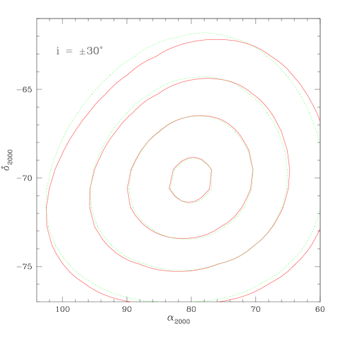
Figure 3: Isodensity contours of test models showing the sensitivity to the direction of inclination. Each test model is represented by 3000 sources distributed according to an exponential disk with $\left\{\alpha_{0},\delta_{0},R,i,\theta\right\}$ = $\left\{80^{\circ},-70^{\circ},1.5,\pm 30^{\circ},135^{\circ}\right\}$. Four logarithmically spaced density levels of 0.0003, 0.001, 0.003, 0.01 deg^-2 are shown. Solid line shows model with $i=-30^{\circ}$, dotted line — model with $i=+30^{\circ}$. The difference is clearly seen, especially in outer contours.

The results of fits to a spherical power-law profile are described in Table 3. There are no significant difference between power-law exponents for various populations: all values are $\approx 2.5-2.6$. The centroid shift for younger populations, present in Table 2, is seen here as well. The underlying distribution, a disk and spheroid together, is described here as a single profile. A power-law disk profile, of course, will have an index $1+\nu$, where $\nu$ is the index for the spherical profile, and therefore some unknown combination of a disk and spheroid makes interpretation difficult. We note that these fits have poorer quality than the exponential fits and probably do not bear on the reality of a spheroidal population. A more independent test for spatially extended population is described below (§4.2).

Table 3: Best fit parameters of power law model.

Region	Parameters
	$\alpha_{0}(^{\circ})$	$\delta_{0}(^{\circ})$	$\nu$
A	80.8	-69.0	$2.60\pm 0.01$
E	80.5	-69.9	$2.52\pm 0.01$
F	80.3	-69.9	$2.59\pm 0.01$
G	80.7	-69.1	$2.65\pm 0.02$
H	80.2	-69.0	$2.55\pm 0.02$
J	80.7	-69.9	$2.56\pm 0.01$
K	80.4	-69.9	$2.59\pm 0.02$

The positional accuracy of distribution centroids ($\alpha_{0}$, $\delta_{0}$) is $\hbox{ \hbox to0.0pt{\raise 1.82986pt\hbox{$<$}\hss}\lower 2.79857pt\hbox{$\sim$} }0.1^{\circ}$.

We compared the results of our fits to similar fits by Hughes et al. (1991), who modeled the distribution of intermediate and old long-period variables (ILPV and OLPV, respectively) with exponential disk and power law models. They found $\nu=1.8\pm 0.1$ and $R=1.6\pm 0.2$ (OLPV), $\nu=1.7\pm 0.1$ and $R=1.7\pm 0.2$ (ILPV). Our results for similar populations (Regions E, F, G and J) imply $\nu\sim 2.5$ and $R\sim 1.4$ kpc. While the scale lengths $R$ are mutually consistent, the best-fit power law exponents differ. Our best fit parameters are larger than the power-law model exponents of Hughes et al. which has $\nu\approx 2.0$.

To summarize, the projected distribution of LMC populations observed by 2MASS is consistent with previous studies. We found the scale length of the LMC disk, $R\sim 1.4-1.5$ kpc, the inclination angle, $i\sim 24^{\circ}-28^{\circ}$, and the direction of the LMC tilt in good agreement with existing estimates.

4 Standard Candle Analysis

We complement our previous analysis (§3) by incorporating photometric distances in addition to our CMD selection. Below, we describe the selection of standard candles, the details of the analysis, and the implications for the structure of the LMC derived from 2MASS photometry.

4.1 Selecting Standard Candles from 2MASS Data

Good standard candles satisfy three conditions: 1) they must be luminous and easily identified; 2) they must be sufficiently numerous and representative of the underlying structure, and 3) they must have small photometric dispersion as a class (that is, small $\sigma_{M}$). In NW00, we argued that stars in Region J of the 2MASS CMD are potentially good standard candles. Being brighter and redder than the RGB tip, most of these stars are carbon-rich thermally-pulsating AGB stars (TP-AGB). Recent data Alves et al. (1998); Wood (1999) suggests that most of these stars exhibit Mira-like variability. The fraction of variables in this region is close to $100\%$, although roughly $25\%$ could be binaries Wood (1999). Here, we will assume that all sources in Region J are carbon-rich long-period variables. Their red colors effectively discriminate against the population of oxygen-rich LPVs, since the latter rarely have $J-K_{s}>1.5$ Hughes & Wood (1990). As long-period variables, these stars follow a linear period-luminosity-color relation (e.g. Feast et al. 1989). The luminosity of these stars can be characterized by their periods or near-infrared colors, and therefore, these stars can be used to probe the structure of the LMC along the line of sight.

The 2MASS sample of C-rich LPVs in the LMC contains 8229 stars. The surface map of Region J is shown in Figure 4.

Figure 4: Density map of CMD Region J. The surface map covers color range from $J-K_{s}=1.5$ to $J-K_{s}=2.0$. Note the well-defined ridge, which suggests a luminosity-color relation for these stars.

The luminosity-color relation for these stars results in the well-defined ridge in the figure. In the absence of the period data, we cannot use standard PL or PC relations to calibrate the intrinsic brightness of these variables. Rather, we have to rely on luminosity-color relation. Figure 5 shows the sample of 79 oxygen- and carbon-rich Miras in the LMC Glass et al. (1990). Magnitude and color of each Mira are averaged over period and plotted on top of 2MASS color-magnitude digram. The luminosity-color relation (shown with the solid line) for 14 carbon Miras in the color interval bounded by vertical dashed lines is

$$<K_{s}>=(-0.99\pm 0.80)<J-K_{s}>+(12.36\pm 1.33),\qquad\sigma=0.38.$$

The average r.m.s is $\sigma\hbox{ \hbox to0.0pt{\raise 1.82986pt\hbox{$<$}\hss}\lower 2.79857pt\hbox{$\sim$} }0.3^{m}$ for $1.4<J-K_{s}<1.7$. Given this LC relation, we may argue that selecting LPVs from a reasonably narrow color range will result in sources with similar luminosities, i.e., standard candles. For our analysis, we choose color interval $1.6<J-K_{s}<1.7$, sufficiently narrow to ensure similar luminosities of our standard candles and sufficiently broad to host enough sources (1385) for statistically meaningful inference.

Figure 5: The sample of 79 oxygen- and carbon-rich Miras from Glass et al. (1990), plotted over the color-magnitude diagram of 2MASS. Magnitude and color of each Mira are converted to CIT photometric system and averaged over the period. Vertical dashed lines show the color range, $1.4<J-K_{s}<1.9$, used for the straight line fit to luminosity-color relation. The best-fit LC relation is indicated with thick solid line.

The ridge-line fit above was based on the average LC relation. From analysis of light curves in Glass et al. (1990), the amplitudes of carbon-rich LPVs are $\Delta K\hbox{ \hbox to0.0pt{\raise 1.82986pt\hbox{$<$}\hss}\lower 2.79857pt\hbox{$\sim$} }0.5$ mag, so one may expect significant broadening of the LC relation due to random phase observations. However, as we will demonstrate below (§4.3), the width of main peak in the apparent luminosity function is only $\sigma\approx 0.2^{m}$, even with random phase observations. This suggests that the phase-average LC relation is much tighter.

4.2 Method

Without prior knowledge of the true source distribution, which is likely to be irregular due to tidal interaction (e.g. Weinberg 2000) or sufficient characterization of the stellar populations to allow a non-parametric density estimation with all of the data, we study the photometric distribution in several fields in the LMC. The fields are located along two great circle arcs passing through the central region of the Cloud: Arc 1, parallel to the line of nodes, and Arc 2, perpendicular to the line of nodes (see Fig. 6).

Figure 6: Locations of selected LMC fields. Field positions follow two arcs: Arc 1 (North-South direction, parallel to the line of nodes), and Arc 2 (East-West direction, perpendicular to the line of nodes). Field numbers are indicated, with arc numbers given in parentheses. Field 3 is the same for both arcs.

The apparent luminosity function can be analyzed in terms of the centroid $\overline{m}$ and the width $2\sigma_{m}$ of the distribution. For a homogeneous standard candle population, the centroid of the distribution measures LMC distance and the width of the distribution gives an estimate of its line-of-sight depth. The error analysis of a standard apparent magnitude-absolute magnitude-distance relation gives

$$\sigma_{m}^{2}\approx\sigma_{M}^{2}+\frac{4.72}{R_{LMC}^{2}}\sigma_{r}^{2}+\sigma_{A}^{2}+\sigma_{ph}^{2},$$ (3)

where $R_{LMC}=50$ kpc is the average distance to the LMC, $\sigma_{M}$ is the intrinsic precision of our standard candles, $\sigma_{A}$ is the variance due to extinction, $\sigma_{r}$ is the geometric depth, and $\sigma_{ph}$ is the photometric error. Equation (3) states that the apparent brightness distribution is the convolution of the spatial density and the intrinsic luminosity function and therefore provides an upper limit to the geometrical depth.

4.3 Results and Interpretation

The brightness distributions of standard candles in selected fields are shown in Figures 7 and 8.

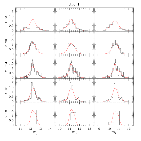
Figure 7: Apparent brightness distribution of selected C-rich Miras in fields along Arc 1. Histograms are normalized raw data, smooth curves are kernel smoothed densities. The bin widths in each histogram are chosen to ensure signal-to-noise ratio of 3 or better. Columns correspond to $J$, $H$, $K_{s}$ bands, rows correspond to fields. Fields and the numbers of C-rich LPVs in the fields are labeled. See Figure 6 for field designations.

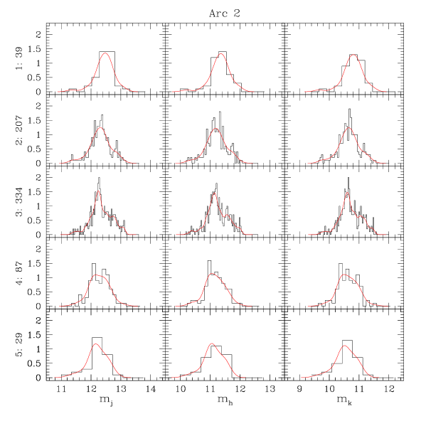
Figure 8: Same as Figure 7, but for fields along Arc 2.

All fields in Figures 7 and 8 exhibit well-defined central peaks corresponding to the midplane of the LMC disk. We immediately notice that the narrowest features in the brightness distributions have widths $\sigma_{m}\approx 0.2^{m}$ (cf. Field 3). This is a direct evidence that our color-selected sources are standard candles at least as good as $\sigma_{M}\approx 0.2^{m}$. In fact, they are even better, because of the additional terms on the right-hand-side in equation (3). This suggests that carbon LPVs in the narrow ($\sim 0.1$ mag) color range are excellent standard candles, even observed at random phases.

4.3.1 Analysis of the Distribution Centroids

The centroids of the distributions are consistent with the inclination of the LMC derived in §3. Since Arc 1 is parallel to the line of nodes, the stars in the fields along this arc should be roughly at the same distance. Hence, we do not expect any drift in the means $\overline{m}$ for stars in these fields. On the other hand, we expect a shift in the mean magnitude for fields along Arc 2, which is perpendicular to the line of nodes. Assuming the Eastern part of the Cloud is closer to us, sources in Eastern fields should be, on average, brighter than their counterparts in Western fields. Figures 7 and 8 confirm the expectations. The magnitude of the effect is shown in Figure 9 for both arcs as the function of the angular distance from the optical center of the bar.

Figure 9: The mean magnitude offset averaged over $J$, $H$, $K_{s}$ bands as the function of the angular distance from the optical center of the bar. The offsets are given relative to the central fields of the corresponding arcs.

To improve the signal-to-noise ratio, we take the average $\overline{m}$ of the mean magnitudes in three bands and plot the resulting averages normalized to the central field of the respective arc. We find that fields along the North-South line have similar mean magnitude, whereas Eastern fields are on average $0.1^{m}$ brighter and Western fields are $\sim 0.2^{m}$ fainter than central bar fields. The magnitude difference is similar to what Caldwell & Coulson (1986) found in their analysis of Cepheids in the Cloud.

Data shown in Figure 9 allow independent determination of the LMC inclination angle. We provide results of two methods: (1) the inclination of the best fit plane to the photometric distance estimate for each field; and (2) the mean inclination of each field paired with the central field. In Method 1, we compute the best fit line through spatial positions of the field centers. The estimates for each arc are $0.9^{\circ}\pm 0.3^{\circ}$ and $42.3^{\circ}\pm 7.2^{\circ}$, respectively. We observe that the inclinations along our Arc 1, as expected, are consistent with zero, while the inclination angles along Arc 2 are consistent with values in Table 2 at $2\sigma$ level. Alternatively, in Method 2 does not presuppose a tilted plane but rather computes the inclination of each field relative to the line of sight through the central field. We then compute the weighted average over all pairs. The resulting inclinations are $1.0^{\circ}\pm 4.1^{\circ}$ and $34.4^{\circ}\pm 2.7^{\circ}$ for the first and second arcs, respectively.

In principle, this magnitude drift could have been produced by a reddening gradient across the Cloud. However, the extinction maps by Oestreicher & Schmidt-Kaler (1996) do not show any systematic change in reddening in the West-East direction across the LMC. In addition, an analysis of the extinction across the entire cloud based on the location of the giant branch reveals little evidence for significant extinction on average outside of the inner square degree Nikolaev & Weinberg (2000). Moreover, if the magnitude drift were indeed due to reddening gradient, it would have had band-dependent signature. The ratios of magnitude offset in $J$, $H$, $K_{s}$ bands would be in direct proportion to the extinction coefficients $A_{J}$, $A_{H}$, $A_{K}$. Since this is not the case, we have to reject this possibility and interpret the drift as the true distance effect.

4.3.2 Shape of the Distributions

Careful study of the density distributions in Figures 7 and 8 shows that some distributions have extended tails. For example, distributions in Fields 3 and 4 clearly show positive skewness. Figure 4 also shows the extension of the central ridge toward fainter magnitudes. To quantify the extended component, we model the distribution of LMC disk sources with a properly centered Gaussian. After subtracting the disk component in the central field (Field 3), we find a secondary, broader distribution which contains approximately 90 sources or about a quarter of the total number in the field. This distribution itself appears to have two distinct components. The strongest peak of this extended component is $0.5$ mag fainter than that of the disk distribution and a weaker peak is roughly $0.8$ mag brighter. In general, the tail toward fainter magnitudes is more pronounced, although the distribution extends to both sides.

Among the factors which could produce the extended component visible in Figures 7 and 8 are: 1) foreground population, 2) source blending, 3) interstellar reddening, 4) population of overtone pulsators, 5) distribution of periods, 6) age/metallicity variations, and 7) spatial density distribution. Foreground population can be rejected because the fraction of Galactic sources in Region J is nearly zero (see Table 1). Interstellar reddening would produce a band-dependent effect (i.e. longer tails in $J$ band than in $K_{s}$ band). We consider each of the remaining five possibilities in detail:

1. Source blending. Considering that the secondary peak runs parallel to the main LC relation (cf. Figure 4), at least one member in the blend must be a carbon star. However, blending a carbon star with an unresolved source would produce a source brighter than the carbon star. This means the secondary peak would be brighter than the main feature, which contradicts to data;

2. Population of overtone pulsators. The question about the pulsation mode of Mira variables seem to have been resolved recently with Miras unambiguously identified as fundamental mode pulsators Wood & Sebo (1996); Wood et al. (1998). It is conceivable, then, that our color-selected sample of standard candles includes a population of first- and higher-overtone LPVs. Based on Figures 7 and 8, this ‘secondary’ population should constitute about $25\%$ of the entire sample, and be fainter by $0.4-0.5^{m}$. We test this possibility by cross-correlating 2MASS data with the sample of Hughes & Wood (1990), which contains fundamental-mode LPVs only. Picking out sources in the color range $1.6<J-K_{s}<1.7$ and plotting the histogram of their $K_{s}$ magnitudes reveals the same extended component, approximately $0.5$ mag fainter than the main peak. Since the feature is present even in the data without overtone pulsators, this explanation has to be rejected;

3. Distribution of periods. Even in case of zero-dispersion PLC relation for C-rich LPVs, the observed magnitude distribution could result from an intrinsic period distribution (in addition to overtone pulsations discussed above). Although this explanation remains a possibility because the physics of these stars remains uncertain in detail, such an effect is not apparent in current theoretical models, which confirms an intrinsic width of the instability strip but not multiple peaks. Conversely, as previously mentioned, the good fit of the primary peak to the disk inclination gives us confidence in a well-defined instability strip and width of this peak is consistent with other pulsators. Alternatively, the pulsation periods depend on mass and metallicity and distribution of periods implies the range of mass, ages and metallicities, and vice versa. Assuming a range of initial AGB masses leads to the range of intrinsic bolometric magnitudes for a single period Marigo et al. (1996). Marigo’s et al. theoretical evolutionary tracks show the difference in a few tenths of a magnitude for carbon Miras at a constant period, depending on the mass of the star. Fitting the apparent luminosity function to these tracks Cole (2000) suggests that the stronger peak may be due to younger ($\sim 0.6$ Gyr) and more massive stars ($2M_{\odot}$), while the broader component is formed by older ($\sim 2.8$ Gyr) and less massive ($\sim 1.2M_{\odot}$) stars. This appears consistent with observations: Frogel et al. (1990) found that carbon stars are present in globular clusters aged 100 Myr to about 3 Gyr and that carbon stars in intermediate-age LMC clusters are a few tenths of a magnitude fainter than those in young LMC clusters. Alves et al. (1998) reported that AGB variables in the intermediate age cluster NGC 1783 are about 0.5 mag brighter at given period than variables in ancient LMC globular cluster NGC 1898. We find two aspects of this possibility to be unsatisfying. First, it does not naturally explain the bright secondary peak. Second, the star formation rate subsequent to the 2.8 Gyr burst would have to be small in order to result in a well-defined feature;

4. Extended density distribution in the LMC. This appears to be the most natural explanation to the observed brightness distributions: it is band-independent, it does not rely on special star formation history, and straightforwardly explains both the brighter and fainter secondary distribution. The distinct feature at fainter magnitudes may be associated with the population kinematically distinct from the disk sources, recently found by Graff et al. (1999). This motivates a detailed kinematic follow-up of the small bright “clump” in the photometric distribution. Based on the offset, this population is 15 kpc from the LMC center and coincident with the intervening population detected by Zaritsky & Lin (1997). The existence of LPVs implies a relatively young population, and the broad area is consistent with tidally stripped material. A future detailed study will attempt to self-consistently model the disk, an extended spheroid component as suggested by Hughes et al. (1991), and test for other distinct features. Regardless of details, the broad photometric distribution suggests that LMC is geometrically thick along the line of sight. From Figures 7 and 8, the average thickness of the LMC is $2\sigma_{m}\sim 0.7^{m}$, which implies a thickness (after deconvolution) of $\sim 14$ kpc (for the LMC distance $R_{LMC}=50$ kpc). This makes the LMC as thick along the line of sight as it is wide across the sky, something which one would naively expect for a dwarf companion in the process of being tidally shredded. In summary, the spatial interpretation of these photometric distributions suggests the LMC consists of a centrally concentrated barred disk and some number of extended distributions, including a spheroid and tidally distorted and possibly stripped populations.

5 Summary

We have analyzed the spatial distributions of several LMC populations, identified in NW00 based on their location in the color-magnitude diagram. Quantitative analysis of the observed distributions includes parametric source-count and a preliminary standard candle analyses. Our major conclusions are:

• Projected star count analyses based 2MASS data yield scale lengths, deprojection-based inclinations, and position angles consistent with previous studies. The near-far degeneracy of the disk orientation is broken by perspective difference. The near side of the Cloud subtends a larger angle in the sky-and this allows us to determine that Eastern side of the disk is closer, in agreement with Cepheid-based results.

• We propose using carbon-rich LPVs in a narrow color range, $1.6<J-K_{s}<1.7$ as standard candles to probe the structure of the LMC along the line of sight. Based on published light curves, their intrinsic magnitudes have a dispersion of $\hbox{ \hbox to0.0pt{\raise 1.82986pt\hbox{$<$}\hss}\lower 2.79857pt\hbox{$\sim$} }0.3^{m}$ including the random phase of the observations. The width of the LMC disk in the observed photometric distribution ($\sigma_{m}\approx 0.2$) suggests that these are excellent standard candles.

• The photometric distribution of our standard candle sample reveals strong central peak with extended tails in both directions, with tail toward fainter magnitudes more pronounced. In the densest field, the distributions in all bands show two secondary peaks, $0.5$ mag fainter and $0.8$ mag brighter than the primary. We interpret the primary peak as due to the midplane of the LMC disk and examine various possibilities which could produce the tails and secondary peaks of observed distribution. We conclude that the photometric distribution of standard candles is most likely caused by a spatially extended stellar component and tidally stripped debris, consistent with a tidally disturbed dwarf companion. It is possible that the distribution reflects the intrinsic period distribution of LPVs but or distinct populations of masses (ages) and metallicities for these stars, but such explanations special populations or evolutionary histories.

• The distribution of apparent magnitudes of standard candles is consistent with tilted geometry derived from star counts. We derive a direct determination of the LMC disk inclination of $42.3^{\circ}\pm 7.2^{\circ}$, consistent with Laney & Stobie (1986) estimate of $45^{\circ}\pm 7^{\circ}$ and with results of Welch et al. (1987), $37^{\circ}\pm 16^{\circ}$. Interpreting the apparent luminosity function as due to real source density, we find evidence of the extended component of the LMC, with a width of approximately 14 kpc (for the LMC distance $R_{LMC}=50$ kpc).

This detection of this thick component implies that LMC may contain a kinematically distinct population as suggested by Graff et al. (1999) and/or an the extended component found by Hughes et al. (1991) and predicted for the tidal interaction with the Milky Way (Weinberg 2000). The existence of such a population will affect the self-lensing models of the LMC in the microlensing studies. These preliminary results suggest a number of projects for short- and long-term follow-up. An improved analysis of the 2MASS sample may be obtained with larger sample of standard candles, or with full three dimensional analysis based on several distinct standard candles using data from the entire survey rather than selected fields (work in progress). Assuming that the extended stars originated in the disk, both populations will appear rotationally supported. However, using the 2MASS photometric distribution as a guide, a combined disk and extended spheroid population should be kinematically separable and these stars are good candidates for future spectroscopic work.

Appendix A Parametric Maximum Likelihood

The expected source density for a bin in the direction ($\alpha_{i}$, $\delta_{j}$) is determined by integrating the LMC density model along the line of sight across the bin. This is given by the following integral:

$$\rho^{exp}_{ij} \propto \int_{0}^{\infty}dt\,t^{2}\int_{\delta_{j}-\Delta\delta/2}^{\delta_{j}+\Delta\delta/2}d\delta\cos\delta\int_{\alpha_{i}-\Delta\alpha/2}^{\alpha_{i}+\Delta\alpha/2}d\alpha\,\rho(t,\alpha,\delta)$$ (A1)

$$\approx \int_{0}^{\infty}dt\,t^{2}\rho(t,\alpha_{i},\delta_{j})\cos\delta_{j}\,\Delta\alpha\,\Delta\delta,$$

where the last equality assumes that the bin size $\Delta\alpha$, $\Delta\delta$ is sufficiently small. We perform the integral in (A1) using 256-point Gaussian quadrature formula, with $20$ kpc and $80$ kpc as the integration limits. The underlying source density $\rho(t,\alpha,\delta)$ is given either by equation (1) or by equation (2). The coordinate transformations for both models follow.

A.1 Exponential Disk

To quantify $\rho(\cdot)$, we introduce the coordinate system $\{x_{0},y_{0},z_{0}\}$ which has the origin at the center of the LMC at $\{t,\alpha,\delta\}=\{R_{LMC},\alpha_{0},\delta_{0}\}$ and has $z_{0}$-axis toward the observer, $x_{0}$-axis antiparallel to the right ascension axis, and $y_{0}$-axis parallel to the declination axis. The coordinate transformations are given by

$$x_{0} = -t\cos\delta\sin(\alpha-\alpha_{0})$$

$$y_{0} = t\sin\delta\cos\delta_{0}-t\cos\delta\sin\delta_{0}\cos(\alpha-\alpha_{0})$$ (A2)

$$z_{0} = R_{LMC}-t\cos\delta\cos\delta_{0}\cos(\alpha-\alpha_{0})-t\sin\delta\sin\delta_{0}.$$

The coordinate system of the exponential disk, $\{x^{\prime},y^{\prime},z^{\prime}\}$, is the same rectangular system as $\{x_{0},y_{0},z_{0}\}$, except rotated about $z_{0}$-axis by the position angle $\theta$ counterclockwise and about the new $x^{\prime}$-axis by inclination angle $i$ clockwise. The coordinate transformations are given by

$$x^{\prime} = x_{0}\cos\theta+y_{0}\sin\theta$$

$$y^{\prime} = -x_{0}\sin\theta\cos i+y_{0}\cos\theta\cos i-z_{0}\sin i$$ (A3)

$$z^{\prime} = -x_{0}\sin\theta\sin i+y_{0}\cos\theta\sin i+z_{0}\cos i.$$

Because our resolution in photometric distance is larger than the disk thickness, the integral in equation (A1) may be simplified by assuming that the exponential disk is infinitely thin, i.e. $z^{\prime}=0$ for all points of the disk. The contribution to the integral is zero everywhere, then, except the point where line of sight intercepts the plane of the disk. The value of $t$ at the intercept, $\overline{t}$, is

$$\overline{t} = -R_{LMC}\cos i\times\left[\cos\delta\sin(\alpha-\alpha_{0})\sin\theta\sin i\right.$$ (A5)

$$\left.+\left(\sin\delta\cos\delta_{0}-\cos\delta\sin\delta_{0}\cos(\alpha-\alpha_{0})\right)\cos\theta\sin i\right.$$

$$\left.-\left(\cos\delta\cos\delta_{0}\cos(\alpha-\alpha_{0})+\sin\delta\sin\delta_{0}\right)\cos i\right]^{-1}.$$

The values of $x_{0}$, $y_{0}$ and $z_{0}$ coordinates at the intercept point follow from equation (A.1). The radius of the intercept point in the plane of the exponential disk is given by

$$r=\sqrt{x^{\prime 2}+y^{\prime 2}}.$$ (A6)

Finally, the expected source density (A1) may be written as

$$\rho^{exp}_{ij}\propto\overline{t}^{2}{\rm exp}(-r/R)\cos\delta_{j},$$ (A7)

where $\overline{t}$ and $r$ are given by equations (A5) and (A6), respectively.

A.2 Power Law Model

Treatment of the spherical power law model is much simpler. Unlike the disk, there is no unique axis of symmetry and one may write the density (2) in the coordinates $t$, $\alpha$ and $\delta$ directly. It is straightforward to verify that

$$r=\sqrt{t^{2}+R_{LMC}^{2}-2R_{LMC}t\left[\cos\delta\cos\delta_{0}\cos(\alpha-\alpha_{0})+\sin\delta\sin\delta_{0}\right]}.$$ (A8)

References

- Alves et al. (1998) Alves, D. et al. 1998, astro-ph/9804003
- Caldwell & Coulson (1986) Caldwell, J. A. R. & Coulson, I. M. 1986, MNRAS, 218, 223
- Cole et al. (1999) Cole, A. A., Wood, K., Nordsieck, K. H. 1999, AJ, 118, 2292
- Cole (2000) Cole, A. A. 2000, private communications
- Feast et al. (1989) Feast, M. W., Glass, I. S., Whitelock, P. A., Catchpole, R. M. 1989, MNRAS, 241, 375
- Feitzinger et al. (1977) Feitzinger, J. V., Isserstedt, J., Schmidt-Kaler, Th. 1977, A&A, 57, 265
- Freeman et al. (1983) Freeman, K. C., Illingworth, G., Oemler, A. 1983, ApJ, 272, 488
- Frogel et al. (1990) Frogel, J., Mould, J., Blanco, V. M. 1990, ApJ, 352, 96
- Gascoigne & Shobbrook (1978) Gascoigne, S. C. B., Shobbrook, R. R. 1978, PASAu, 3, 285
- Glass et al. (1990) Glass, I. S., Whitelock, P. A., Catchpole, R. M., Feast, M. W., Laney, C. D., 1990. S. Afr. Astron. Obs. Circ., 14, 63
- Graff et al. (1999) Graff, D. S., Gould, A. P., Suntzeff, N. B., Schommer, R. A., Hardy, E. 1999, astro-ph/9910360
- Hughes & Wood (1990) Hughes, S. M. G. & Wood, P. R. 1990, AJ, 99, 784
- Hughes et al. (1991) Hughes, S. M. G., Wood, P. R., Reid, N. 1991, AJ, 101, 1304
- Kunkel et al. (1997) Kunkel, W. E., Demers, S., Irwin, M. J., Albert, L. 1997, ApJL, 488, L129
- Laney & Stobie (1986) Laney, C.D. & Stobie, R. S. 1986, MNRAS, 222, 449
- Marigo et al. (1996) Marigo, P., Bressan, A., Chiosi, C. 1996, A&A, 313, 545
- McGee & Milton (1966) McGee, R. X. & Milton, J. A. 1966, Aust. J. Phys., 19, 343
- Nikolaev & Weinberg (2000) Nikolaev, S. & Weinberg, M. D. 2000, astro-ph/0003012 (NW00)
- Oestreicher & Schmidt-Kaler (1996) Oestreicher, M. O. & Schmidt-Kaler, Th. 1996, A&AS, 117, 303
- Schmidt-Kaler (1977) Schmidt-Kaler, Th. 1977, A&A, 54, 771
- Schmidt-Kaler & Gochermann (1992) Schmidt-Kaler, Th. & Gochermann, J. 1992, in Variable Stars and Galaxies, ASP Conference Series, Vol. 30, edited by B. Warner, p. 203
- Schommer et al. (1992) Schommer, R. A., Olszewski, E. W., Suntzeff, N. B., Harris, H. C. 1992, AJ, 103, 447
- Searle et al. (1980) Searle, L., Wilkinson, A., Bagnuolo, W. G. 1980, ApJ, 239, 803
- de Vaucouleurs (1955) de Vaucouleurs, G. 1955, AJ, 60, 126
- de Vaucouleurs (1957) de Vaucouleurs, G. 1957, AJ, 62, 69
- de Vaucouleurs (1980) de Vaucouleurs, G. 1980, PASP, 92, 576
- de Vaucouleurs & Freeman (1973) de Vaucouleurs, G. & Freeman, K. C. 1973, Vis. Astron., 14, 163
- Weinberg (2000) Weinberg, M. D. 2000, ApJ, in press.
- Welch et al. (1997) Welch, D. L., McLaren, R. A., Madore, B. F., McAlary, C. W. 1987, ApJ, 321, 162
- Wood & Sebo (1996) Wood, P. R. & Sebo, K. M. 1996, MNRAS, 282, 958
- Wood et al. (1998) Wood, P. R. et al. 1998, IAU Symp. 191
- Wood (1999) Wood, P. R. 1999, private communications
- Zaritsky & Lin (1997) Zaritsky, D. & Lin, D. N. C. 1997, AJ, 114, 2545