QSOs and Absorption Line Systems Surrounding the Hubble Deep Field

Abstract

We have imaged a $45\arcmin\times 45\arcmin$ area centered on the Hubble Deep Field (HDF) in $UBVRI$ passbands, down to respective limiting magnitudes of approximately $21.5,22.5,22.2,22.2,{\rm and\ }21.2$. The principal goals of the survey are to identify QSOs and to map structure traced by luminous galaxies and QSO absorption line systems in a wide volume containing the HDF. The area surveyed is $400$ times that of the HDF, and $40$ times that of the HDF Flanking Fields. We have selected QSO candidates from color space, and identified 4 QSOs and 2 narrow emission-line galaxies (NELGs) which have not previously been discovered, bringing the total number of known QSOs in the area to $19$. The bright $z=1.305$ QSO only 12′ away from the HDF raises the northern HDF to nearly the same status as the HDF-S, which was selected to be proximate to a bright QSO. About half of the QSO candidates remain for spectroscopic verification.

Absorption line spectroscopy has been obtained for $3$ bright QSOs in the field, using the Keck 10m, ARC 3.5m, and MDM 2.4m telescopes. Five heavy-element absorption line systems have been identified, 4 of which overlap the well-explored redshift range covered by deep galaxy redshift surveys towards the HDF. The two absorbers at $z=0.5565$ and $z=0.5621$ occur at the same redshift as the second most populated redshift peak in the galaxy distribution, but each is more than $7h^{-1}$Mpc (comoving, $\Omega_{m}=1$, $\Omega_{\Lambda}=0$) away from the HDF line of sight in the transverse dimension. This supports more indirect evidence that the galaxy redshift peaks are contained within large sheet-like structures which traverse the HDF, and may be precursors to large-scale “pancake” structures seen in the present-day galaxy distribution.

1 Introduction

Deep galaxy redshift samples are permitting a new and often surprising view of the Universe at much younger epochs, and into which the role of gas, both hydrogen and processed, via QSO absorption line systems can be incorporated. Only recently, and with the help of the 10-m Keck telescopes, have deep galaxy redshift surveys been able to measure properties of galaxies at some of the redshifts ($2.5\lesssim z\lesssim 4.5$) which have been easily accessible to absorption line studies for over three decades. Combining the study of QSO absorbers and galaxy surveys has the potential to greatly enhance our understanding of the formation and evolution galaxies as well as the large-scale structures which typically contain them. For example, even if galaxies and absorbers are closely related, biasing, which plays an important role in deciphering structure formation, is expected to be different for for galaxies, QSOs, absorbers, and the various classes of each (e.g.  Demiański & Doroshkevich, 1999; Cen et al., 1998; Fang & Jing, 1998; Quashnock & Vanden Berk, 1998; Bi & Fang, 1996).

A generic result of the deep galaxy pencil-beam surveys is that half or more of the galaxies measured tend to lie in very narrow redshift “spikes” which are present to redshifts of at least $z=1$ (Cohen et al., 1996a, b) and are often found at much higher redshifts ($z\approx 3$) in the “dropout” surveys (Steidel et al., 1998; Adelberger et al., 1998). The number density, redshift spacing, density enhancements, velocity dispersions, and morphological mixtures, all support the hypothesis that these structures in redshift space are parts of the precursors to present-day galaxy superclusters and walls (Cohen et al., 1996a, b). This evidence is mostly circumstantial so far, since the deep pencil-beam surveys cover only very small (typically 50 sq. arcmin. or less) disjoint areas of the sky. Additional but shallower redshift surveys have been carried out in narrow fields adjacent to at least one deep pencil beam survey, which have supported the the idea that the redshift structures are coherent in the transverse spatial dimension on scales up to at least a degree, and for redshifts up to at least $z\approx 0.4$ (Cohen et al., 1999). Extending this type of survey to deeper redshifts is difficult not only due to the faintness of the galaxies, but in the redshift range $1.2\lesssim z\lesssim 2$ there is a lack of redshifted galaxy spectral features available at optical wavelengths. It is a highly desirable but currently difficult goal of future redshift surveys to cover both larger areas and a more complete redshift range. QSO absorption line systems offer a means of efficiently extending these studies to wider volumes and higher redshift, which is the aim of the program described here.

The approach is to search for intervening absorption line systems in the spectra of QSOs at small angular separations. The selection function for heavy-element QSO absorption line systems, identified mainly by C iv $\lambda$1550Å and Mg ii $\lambda$2799Å doublet transitions, is luminosity independent, and limited at high redshift only by the emission redshift of the backlighting QSOs. In optical spectra Mg ii lines can be detected from redshifts of $z\approx 0.15-2.0$ and C iv lines from $z\approx 1$ to over 4. Absorption surveys towards groups of QSO sightlines have been successfully used to trace structure in three dimensions at high redshift (Crotts, 1985, 1989; Jakobsen & Perryman, 1992; Foltz et al., 1993; Elowitz et al., 1995; Dinshaw & Impey, 1996; Williger et al., 1996; Vanden Berk et al., 1999; Impey et al., 1999). A few QSOs have also been observed directly within the areas covered by the galaxy surveys, and their spectra have revealed absorption line systems that very often lie within the redshift peaks defined by the galaxies (Steidel et al., 1998). These studies have demonstrated the utility of absorption line systems in probing large-scale structure both in radial and angular dimensions, and of using large-scale structure studies to decipher the relationship between galaxies and absorbing gas.

QSOs bright enough to use for 3-dimensional absorption line studies generally have a high enough angular density so that suitable groups can be found in virtually any field of sufficiently high galactic latitude. For example, most UVX QSO surveys reveal a density of about 30 QSOs per sq. degree to a limiting magnitude of $B\leq 21$ (e.g.  Zhan et al., 1989), which is a practical limit for absorption line surveys with 4-m class telescopes. To take full advantage of this technique, one should select fields in which deep galaxy redshift surveys have also taken place. The galaxy and absorber surveys are then complementary: the galaxies provide the redshift locations and velocity dispersions of structures, while the absorbers can be used to quickly and efficiently widen the survey to larger areas and additional redshift ranges, and probe the otherwise invisible structure of the gas.

The Hubble Deep Field (HDF; Williams et al., 1996) is the site of one of the most complete and comprehensive sets of deep redshift surveys, with over $300$ measured redshifts in an area of only $\approx 50$ sq. arcmin. (Cohen et al., 1996a; Steidel et al., 1996; Lowenthal et al., 1997; Guzmán et al., 1997; Phillips et al., 1997; Hogg et al., 1998). The measured redshifts lie in the range $z\lesssim 1.3$ and $z\gtrsim 2.0$, with a gap between $1.3$ and $2.0$ due to restrictions of optical spectroscopy. We have chosen the area surrounding the Hubble Deep Field for our initial QSO/absorber study because of the large and continuing amount of research devoted to this sightline, and because it is easily accessible not only by northern-hemisphere telescopes, but also to the Hubble Space Telescope (HST) which can be used for follow-up observations of the low-redshift Ly $\alpha$  systems. Indeed, this latter approach is the primary justification for the construction of the Hubble Deep Field South, and a survey similar to ours for additional QSOs in that direction of the sky is currently taking place (Teplitz et al., 1998). Liu et al. (1999, hereafter LPIF) recently carried out a QSO survey in the one square degree surrounding the HDF, and found 30 QSOs brighter than $B=21$. While the LPIF survey and ours have similar goals and survey depths, ours uses 5-band photometry (LPIF used only $U,B,{\rm and\ }R$ bands) to search for high-redshift QSOs, and we have started QSO absorption line follow-up spectroscopy. Comparisons of the two surveys will be made when appropriate. In this paper we present our initial results on the QSO survey towards the HDF (there are no reasonably bright QSOs inside the HDF itself), and our preliminary absorption line study of 3 of the QSO lines-of-sight. The imaging observations and photometry, QSO candidate selection and verification, and QSO absorption spectroscopy, are presented in § 2, § 3, and § 4 respectively. We discuss the distributions of the QSOs and absorbers relative to the galaxy redshift sample in § 5. A summary is given in § 6.

2 $U,B,V,R,I$ Imaging and Photometry

2.1 Observations and Image Reduction

Images centered on the Hubble Deep Field were taken at McDonald Observatory using the Prime Focus Camera (PFC) mounted on the 0.76 m telescope. The PFC is a dedicated prime focus (f/3.0) corrector with a $2048\times 2048$ Loral Fairchild CCD, which covers an area of $46.25\times 46.25$ sq. arcminutes (a plate scale of $1.355$ arcsec$/$pixel). One CCD field, centered on the HDF, was imaged many times in each of the five filters of the Bessel $UBVRI$ system. Small ($\sim 50$ pixel) offsets were made between each of the exposures to facilitate the removal of CCD chip defects and cosmic ray events.

The observations were made on several nights in late February and early March, 1998. The seeing was exceptionally good on two of the nights, yielding point spread functions with typical FWHM less than 2 pixels. These were also the only photometric nights, such that the standard star observations were useful for absolute photometric calibrations. About half of the images in each band were taken in these conditions. The seeing was substantially worse during the other nights, and it turned out that the co-addition of frames taken on those nights did not improve the image depths enough to justify the loss of morphological information and close-source separation. The primary goal of the QSO search is to identify QSOs bright enough for absorption line system spectroscopy follow-up, so the marginal improvement in magnitude limits is not ultimately important.

The raw images were reduced using a package of IRAF scripts written by Inger Jørgensen specifically to reduce McDonald PFC imaging data. Individual science frames were corrected for bias level, differential shutter open time, flat fields, and illumination gradients. Science frames in each band were co-added taking into account seeing, bad pixels, background level, and noise in each frame. The total exposure times and FWHM for the final coadded science images is given in Table 1.

2.2 Photometry

Standard star observations were taken each night the sky appeared to be photometric. The photometric stability was acceptable on only two of the nights. Typically $4-5$ Johnson-Kron-Cousins $UBVRI$ standard star fields from the list of Landolt (1992) were observed each night at high and low airmasses. The standard star frames were reduced in the same way as the science frames (but with no coaddition). Aperture photometry was performed on all of the standard stars in the frames, and an aperture correction was determined for each filter.

Zero point offsets ($u_{0},b_{0},v_{0},r_{0},i_{0}$), extinction coefficients ($u_{1},b_{1},v_{1},r_{1},i_{1}$), and color corrections ($u_{2},b_{2},v_{2},r_{2},i_{2}$) were determined for the two photometric nights, by interactively fitting the parameters of sets of equations like those below. The equations relate the aperture-corrected instrumental magnitudes ($u,b,v,r,i$) to the standard Johnson-Kron-Cousins magnitudes ($U,B,V,R,I$), the airmass of the observations ($X_{u},X_{b},X_{v},X_{r},X_{i}$), and a color term:

$$u = U+u_{0}+u_{1}\times X_{u}+u_{2}\times(U-B)$$ (1)

$$b = B+b_{0}+b_{1}\times X_{b}+b_{2}\times(B-V)$$ (2)

$$v = V+v_{0}+v_{1}\times X_{v}+v_{2}\times(V-R)$$ (3)

$$r = R+r_{0}+r_{1}\times X_{r}+r_{2}\times(V-R)$$ (4)

$$i = I+i_{0}+i_{1}\times X_{i}+i_{2}\times(R-I)$$ (5)

Systems of equations with many different color terms were fit, since not all science objects were detected in every co-added image. The equations were transformed to yield functions for each of the standard magnitudes. The coefficients varied slightly between the two nights, so separate transformations were applied to the data taken on each of the nights. No correction was made for Galactic reddening, since the direction towards the HDF has a very small reddening factor (Williams et al., 1996).

Objects in the co-added science frames were detected, and their fluxes measured, using the program SExtractor (Bertin & Arnouts, 1996). SExtractor determines the background, detects objects, deblends multiple sources extracted as single objects, measures magnitudes, and discriminates between point-like and extended objects. The program parameters were adjusted so that all objects clearly identified as separate objects by eye were detected and deblended with SExtractor. The SExtractor “best estimate” (using either adaptive aperture or corrected isophotal photometry; Bertin & Arnouts, 1996) of the total flux for each object, was used for magnitude calculations. SExtractor was also run on the standard star frames in order to compare the aperture-corrected and SExtractor magnitude estimates. There was a small ($<3\%$) offset between the two estimates for the standard stars, which did not appear to be magnitude dependent; this offset was applied to the SExtractor magnitudes of the science objects.

An effective airmass for each co-added image was determined by fitting a line to the individual science frame airmasses vs. the instrumental magnitude differences between the co-added frame and the individual frames. The effective airmass (the $y$-intercept of the line fit) for each co-added image was used in the photometric transformation equations.

Science objects were matched on all co-added frames in which they were detected. The final standard magnitude determinations were made for each science object, using the transformation equations, including the color term if possible. If an object was detected in only one frame (for example, faint objects in the $R$ band image, or objects close to a non-overlapping frame edge), no color term was applied.

Uncertainties in the magnitude estimates are given by SExtractor, based upon the flux and extent of the object, and the background variance. These estimates agreed well with uncertainties based upon variations among individual science frames, except for saturated objects. Stars become saturated in our images at approximately $U=12.3,\ B=14.5,\ V=13.8,\ R=14.1,\ {\rm and}\ I=14.1$. We have used the SExtractor estimates for the magnitude uncertainties except for objects brighter than the saturation level, which we simply flagged as “saturated”. The magnitude uncertainties, shown in Fig. 1, reach the 10% level at $U=20.1,\ B=21.3,\ V=21.1,\ R=21.1,\ {\rm and}\ I=20.2$.

Aside from the statistical uncertainties, there may be systematic uncertainties in the magnitude estimates due to a variety of possible causes. For our purposes, systematic uncertainties are not worrisome as long as the stellar locus is well defined by the measured colors, and outliers can be easily identified. However, accurate magnitudes in an absolute sense are necessary for other uses of the data, and for comparison with other studies. To check this, we have compared our $UBR$ magnitudes with those of LPIF (who did not take observations in the $V$ or $I$ bands), for objects common to the two lists. The $B$ and $R$ band measurements in each set are not significantly different, however, our measured $U$ magnitudes are brighter on average by 0.13 mag, which is about 4 standard errors of the mean away from no difference in the $U$ measurements. The vast majority of the objects used for comparison are fainter than $U=20.1$, the 10% uncertainty level of our $U$ band data, which may account for the larger difference. It is also possible that since all of our $U$ band observations were done on a single night, the difference can be attributed to uncorrected sky variations. In any case, the color-color diagrams (§ 3) appear to be in good agreement with those of other studies, and we have not applied additional photometric corrections.

2.3 Astrometry

Astrometry was performed by comparing the pixel coordinates (determined using SExtractor) of stars in our field to the J2000 equatorial coordinates given in the HST Guide Star Catalog. About 90 GSC stars appear in the co-added images. Tasks in the IRAF imcoords package were used to fit a 2-dimensional polynomial function to the pixel/equatorial coordinates. The r.m.s. of the residuals was less than $0.5$ arcseconds in both the $x$ and $y$ pixel dimensions for each co-added image.

2.4 Star-Galaxy Separation

Discrimination between point-like or extended objects is a serious issue for our dataset, given the fairly large pixel size ($1.355\arcsec/$pix). The method we used was based upon the “stellarity index” produced by the SExtractor neural-network classifier (Bertin & Arnouts, 1996). Each object detected in a co-added image was assigned a number between 0 and 1, which represents the confidence that an object is stellar. The stellarity index match for objects detected in multiple bands was quite good. For example, for objects detected in both the $U$ and $R$ band, the indices matched to within 0.1 for more than 75% of the objects, although the correlation degrades with fainter magnitudes. For multiply detected objects, the indices were weighted by the inverse of the squared magnitude uncertainties, then averaged over all the detections. We used an index $\geq 0.6$, because this included a large number of objects without noticeably increasing the width of the stellar locus in the color-color diagrams. In addition, all but one of the confirmed stars and QSOs from LPIF are selected with this cut.

2.5 The Object Catalog

The final imaging catalog contains 10647 objects detected in at least one band, 1516 detected in all 5 bands, and 1836, 4033, 5681, 8736, and 7841 objects detected in the $U,\ B,\ V,\ R,\ {\rm and}\ I$ bands respectively. There are 2147 objects classified as stellar, or about 20% of the total number of objects. Objects selected as QSO candidates will be presented in the next section, but the full catalog is likely to be useful for other studies, particularly because the survey area contains and surrounds the HDF. The full object catalog containing coordinates, magnitudes, uncertainties, and stellarity indices for all of the detected objects, may be obtained by contacting the authors.

3 QSO Candidate Selection and Verification

3.1 Selection of QSO Candidates

QSO candidates were selected based upon their locations in color space. In order to maintain a reasonably high efficiency of QSO selection, the candidates should clearly be located well outside of the stellar locus, and in regions of color space which QSOs are known to occupy at a relatively high density. The simplest selection criterion is to make one or two-dimensional cuts in two-color spaces. For example, QSOs with redshifts up to $\sim 2.2$ can be found with good efficiency by selecting objects with $U-B<-0.3$. At various redshifts, strong features in QSO spectra, such as the onset of the Ly $\alpha$ forest, move into and out of different photometric passbands. Thus QSO colors can be strongly dependent on redshift, and various color space cuts are most efficacious over select ranges of redshift. Automated but more complex outlier selection techniques have been tried in other studies (e.g.  Newberg & Yanny, 1997; Warren et al., 1991), which are appropriate for large surveys for which it is impractical to check every candidate. Our sample is small enough to check each outlier individually, and our goal is not to identify a complete sample of QSOs, so color space cuts, based in part on results from past studies, are adequate for our purposes.

To select the search regions, two-color diagrams were plotted for all unsaturated objects classified as stellar, with magnitudes brighter than the 10% uncertainty level (Fig. 2). For the ($U-B)/(B-V$) diagram, we also plotted all of the available colors of QSOs in the catalog of Véron-Cetty & Véron (1996). Based on the location of the stellar locus and the known QSOs, cuts in ($U-B)/(B-V$) color space were made to select candidates from our imaging catalog. An historically successful method for selecting QSOs up to $z\lesssim 2.2$ is to select objects with $U-B\leq-0.3$ – the so-called “UV-excess” method. This also appeared to be a good cutoff for our dataset, as seen in Fig. 2. In addition, a large fraction of the QSOs plotted from the Véron-Cetty & Véron catalog could have been selected with a $B-V\leq 0.35$ cut, which includes only a small part of the stellar locus (mostly A-stars). These combined cuts in the ($U-B)/(B-V$) plane are the “UVX” selection method. UVX candidates with $B-V>0.6$ are often identified as compact narrow emission line galaxies (NELGs) instead of QSOs. Few of our candidates exceed this limit, so we have not used it as a selection criterion. UVX candidates were divided into “bright” and “faint” sets, depending on whether the $U,B,\ {\rm and}\ V$ magnitudes were brighter or fainter than the 10% uncertainty levels. It is assumed that the “bright” candidates have a higher fraction of true QSOs, due to their better photometric accuracy. The UVX candidates that have not been spectroscopically confirmed are listed in Table 3.

Other cuts in color space, mainly aimed at locating higher-redshift QSOs, have been explored in other studies (e.g.  Irwin et al., 1991; Hall et al., 1996). The number density of QSOs with $z>3$ to the limits of our survey is only about $\sim 5$ per square degree (e.g.  Hall et al., 1996), but even one high-redshift QSO in the direction of the HDF would be valuable for absorption system studies. Hall et al., using a filter set similar to ours, successfully used cuts in color space to identify QSOs up to $z=4.33$. We have adopted several of their selection criteria, with slight modifications, in order to search for higher-redshift candidates in our catalog. These cuts are based on the ($U-V)/(V-R$), ($B-V)/(V-R$), and ($B-R)/(R-I$) two-color diagrams, and usually include objects which are red in the first color and blue in the second. In addition, we have added a cut in the ($U-B)/(B-V$) plane for objects red in $U-V$ which are also blue in $B-V$. The color selection criteria are shown in Fig. 2 and listed in Table 2. The cuts are set at reasonable values designed to run close to the stellar locus without introducing a large fraction of stars. We call these criteria collectively the “high-$z$” selection methods. As with the UVX selection, we have divided the high-$z$ sample into “bright” and “faint” sets, according to the 10% magnitude uncertainty levels. Because larger photometric errors in the faint set can cause a large number of non-QSOs to be selected as candidates, we kept only those faint high-$z$ candidates which passed as candidates using more than one two-color cut. As expected, the high-$z$ selection did not produce as many QSO candidates as the UVX selection. The high-$z$ candidates which have not been spectroscopically identified are listed in Table 4.

3.2 Spectroscopic Candidate Verification

The initial candidate verification was done as a poor-weather contingency program in April 1998 using the McDonald Observatory 2.7m telescope and Large Cass Spectrometer (LCS). All $7$ of the QSO candidates we observed in this run have also been observed by LPIF, and the $4$ QSOs and 1 NELG we confirmed in this run were also identified by them. A fifth candidate (J123800+6213) also turned out to be a QSO, but the S/N level in our spectrum was too low to identify it as such. For a second verification run in March 1999, we had the advantage of the published QSO list of LPIF, and so were able to avoid candidates which had already been observed. Our candidate list contained many UV-excess objects and high-$z$ candidates not in any of the lists of LPIF. We used the McDonald 2.7m and IGI spectrograph to observe $11$ candidates, which yielded 4 QSOs and 2 NELGs.

All of the spectra were reduced using standard techniques and tasks in IRAF. Bias level and flat field corrections were applied, then the spectra were optimally extracted (Horne, 1986), wavelength calibrated, and co-added. A sensitivity correction was applied to give an indication of the relative spectral shapes, but the spectra were not flux calibrated. The final reduced, co-added, calibrated QSO and NELG spectra are shown in Fig. 3.

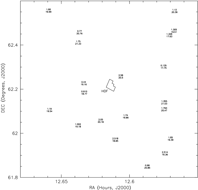
Figure 5: Celestial coordinate positions (J2000) of QSOs identified within our survey area. The QSOs are labeled by their redshifts and $B$ magnitudes. The location of the HDF WFPCII area is indicated.

In total, we observed $18$ QSO candidates, of which $9$ are QSOs, $1$ is an AGN, $2$ are narrow-emission-line galaxies, $4$ are stars, and $2$ remain unidentified. An additional 19 objects in our candidate list were observed by LPIF, $9$ of which are QSOs, and $10$ of which are are stars. One QSO from the LPIF list, J123622+6215, was not selected as a candidate by us, since it has a stellarity index of only $0.37$ caused by blending with a fainter object. The QSOs and NELGs confirmed in our program and those confirmed by LPIF in our survey area, are listed in Table 5. The identified stars are listed in Table 6. There are 16 more bright UV-excess candidates in our list which we have not observed spectroscopically, and which do not appear in the candidate list of LPIF. The unconfirmed UVX QSO candidates are listed in Table 3, and the unconfirmed high-$z$ candidates are listed in Table 4. The redshift distribution of the identified QSOs is shown in Fig. 4, and the coordinate positions are shown in Fig. 5.

While our goal is not a complete survey of QSOs in the area, it is useful to compare the density of QSOs near the HDF to other QSO surveys. Including the QSOs found by us and by LPIF in the $\sim 0.56$ sq. deg. area surrounding the HDF, there is a total of $17$, or roughly $30$ per square degree down to a limiting magnitude of $B=21$. This would be in good agreement with the densities found in several other faint UVX surveys (e.g.  Koo & Kron, 1988; Zhan et al., 1989), which find roughly $30$ per sq. deg., except that we have a remaining 32 unidentified candidates with $B\leq 21$. Applying our UVX success rate (just over 50%, including the results of LPIF) to the remaining 32 UVX candidates with $B\leq 21$, we expect about another $16$ QSOs in our candidate list. Many of the remaining UVX candidates lie close to the $U-B$ and $B-V$ selection limits, and some lie in the region more heavily populated by NELGs, so it is doubtful that the efficiency for the remaining candidates will be as high as $50\%$. Assuming an efficiency only half this ($25\%$) we would reasonably expect about another $8$ QSOs, making the UVX QSO density about $45$ per sq. deg. to $B\leq 21$. While this is significantly higher than most previous studies, the density is in good agreement with Hall et al. (1996) who also noted that the density they found (in separate survey areas) was surprisingly high. The discrepancy may be due to differences in CCD vs. photographic detection techniques, some other selection difference, or real differences in the QSO number density, but the issue is unresolved. In any case, we conclude that our candidate selection is both relatively complete and efficient, and more than adequate for our purposes.

4 QSO Absorption Line System Spectroscopy

The principal goal of the QSO survey is to provide targets for higher-resolution follow-up spectroscopy in order to locate QSO absorption line systems near the HDF. After our first verification run, we identified 4 bright QSOs. Spectra suitable for absorption system searches were obtained for 3 of them: J123414+6226 ($z=1.326$), J123402+6227 ($z=1.305$), and J123637+6158 ($z=2.518$). One of these (J123414+6226) was bright enough to observe at very high resolution using the Keck HIRES spectrograph (Vogt et al., 1994). QSOs J123414+6226 and J123402+6227 are separated by only 112 arcsec. The observing logs for the higher resolution spectra are summarized in Table 7.

The three QSO spectra were searched for absorption lines using the methods described by Vanden Berk et al. (1999). Briefly, a continuum is fit to the spectrum, the flux spectrum and error arrays are normalized by the fit, then convolved with a normalized line-spread-function profile to produce an “equivalent-width” array. Absorption features having a significance level above 3$\sigma$ were flagged, then measured by fitting Gaussian profiles which yield observed line centers, equivalent widths, and their associated uncertainties. The lines were identified with ionic transitions and redshifts based upon the line positions, strengths, and presence of corroborating lines. In the final line list, only lines with a significance level greater then $4.5\sigma$ were kept, unless the line could be identified with a transition occurring in a system identified with more significant lines. The absorption lines are listed in Table 8 and marked on the QSO spectra plots in Figs. 6–8.

Not counting Ly $\alpha$  forest lines, a Milky Way ISM system, and a BAL system, we have identified 5 heavy-element absorption line systems in the three QSO spectra – two each in J123414+6226 and J123637+6158, and one in J123402+6227. The systems in the Keck spectrum of J123414+6226 are at $z=0.28159$ and $z=0.55649$, and both are Mg ii doublet systems. Both systems would be classified as “weak” since their equivalent widths are less than $0.3$Å (Churchill et al., 1999). The system in the ARC/MDM spectrum of J123402+6227 is at a redshift of $z=0.5621$. The line widths are somewhat uncertain since they lie on the blueward edge of the QSO C iii] $\lambda 1909$ emission line, but the line centers and relative equivalent widths are consistent with a Mg ii doublet. There is another possible Mg ii doublet in this spectrum at $z=0.5478$, but we list it only as a candidate, since the doublet ratios are inconsistent, and one line falls below our $4.5\sigma$ completeness limit. No significant lines were detected in the red spectrum of the QSO, but the $4.5\sigma$ lower equivalent width limit of this spectrum, $\sim 1.3$Å, is relatively insensitive. The two systems in the MDM spectrum of J123637+6158 are at $z=0.7913$ and $z=1.8895$, and are identified by a Mg ii and C iv doublet respectively. The spectrum also shows a rich Ly $\alpha$  forest ranging from $2.15<z<2.52$, and a broad absorption line system near $z=2.38$, seen in both Ly $\alpha$  and C iv absorption. Since the BAL phenomena is likely to be unrelated to intervening galaxies (Turnshek, 1984), we have not included it in the analysis of § 5.

5 Comparison With the HDF Galaxy Redshift Distribution

There are so far about $300$ published galaxy redshifts towards the HDF, which come mainly from the surveys of Cohen et al. (1996a); Steidel et al. (1996); Lowenthal et al. (1997); Guzmán et al. (1997); Phillips et al. (1997), and Hogg et al. (1998). The galaxy redshifts measured towards the HDF lie within two redshift ranges, $0\lesssim z\lesssim 1.3$ and $2.9\lesssim z\lesssim 3.6$. There are few measured redshifts between these ranges, due to the lack of prominent spectral features observable at optical wavelengths. QSOs are observable over this entire redshift range, but our highest confirmed QSO has a redshift of $z=2.58$. Absorption systems are detectable at wavelengths above the atmospheric cutoff at $z\gtrsim 0.15$ for Mg ii doublets. Thus the distributions of galaxies, QSOs, and absorbers can be compared within overlapping redshift ranges.

The redshift distribution of the galaxies towards the HDF up to $z=2$ is shown in Fig. 9, and the redshifts of the individual QSOs and absorbers are superimposed. The galaxy distribution is characterized by sharp peaks which contain most of the galaxies. We have defined redshift peaks in a manner similar to Cohen et al. (1996b). The statistical significance parameter, $X_{max}$, is defined as the maximum absolute number of standard deviations the number count in a peak lies from the mean count, found after varying the count histogram bin sizes and locations (Cohen et al., 1996b). A group of galaxies is considered a peak if the group contains at least 5 galaxies, and has an $X_{max}\geq 5$. At least 8 distinct peaks are identified this way at redshifts 0.087, 0.319, 0.455, 0.475, 0.515, 0.559, 0.847, and 0.962, which are marked by dots on Fig. 9. This list includes 5 of the 6 peaks identified by Cohen et al. (1996b), excluding the peak at 0.679 which we find has 7 members but an $X_{max}$ of only $3.9$. Many less significant peaks may also be present. The velocity widths of the peaks are typically $\sigma_{v}\approx 300$km/s. If these structures are the precursors to walls seen in the local universe, as suggested by Cohen et al. (1996b), some of the QSOs and absorbers in the surrounding volume are likely to be contained within these structures. Of the 19 QSOs and 1 AGN, few appear to be coincident with any of the strong galaxy peaks, but several have redshifts close to possible smaller galaxy groups (Fig. 9). The measured redshifts of QSOs can vary by over 1000km/s depending on what emission lines are used and how they are measured (e.g.  Tytler & Fan, 1992). For this reason, QSOs are not ideal for tracing structure on scales less than a few hundred km/s, and any matches between galaxy peak and QSO redshifts would be uncertain.

Redshifts for absorption line systems, on the other hand, can be measured very accurately, even with relatively low-resolution absorption spectra. Of the four absorbers which lie in the well-sampled galaxy redshift range ($z\lesssim 1.3$), two have redshifts coinciding with the second most populated peak in the galaxy distribution at $z\approx 0.559$, one system at $z=0.7913$ lies near a possible weaker galaxy group, and one at $z=0.2816$ does not appear to lie near any galaxy feature. The eight galaxy peaks occupy a total velocity path of about $4800$km/s between $0<z\leq 1.3$ (assuming $600$km/s per peak) or about $2\%$ of the total velocity path, so the random binomial probability of finding two or more out of 4 absorption systems in any of the peaks is about $0.2\%$. Thus it is reasonable to assume that at least some of the absorption line systems are physically related to the peaks in the galaxy distribution.

If the absorbers at $z=0.559$ are parts of the same structure that contains the galaxies, then the galaxy structure extends at least as far as the HDF and absorber transverse separations. For an $\Omega_{m}=1$, $\Omega_{\Lambda}=0$ ($\Omega_{m}=0.3$, $\Omega_{\Lambda}=0.7$) universe, the comoving transverse separations of the QSO absorbers and HDF are $7.9$ ($9.6$) and $8.5$ ($10.4$) $h^{-1}$Mpc. The inclination angle of a hypothesized sheet containing the galaxies and absorbers to the line of sight would likely be less than $30$ degrees, given that each absorber is about one velocity dispersion width ($\approx 460$km/s) from the mean redshift of the galaxy peak, and on opposite sides. Even for fairly large inclination angles, we would expect absorption members of the sheet to lie close to the redshift of the galaxy peak at this transverse separation, since the velocity width of the peak translated into a comoving width is $\approx 3.7$ ($5.3$) $h^{-1}$Mpc at $z=0.559$. At this preliminary stage, the combined galaxy and absorption data are consistent with the suggestion by Cohen et al. (1996a, b) that this structure and those containing other galaxy peaks are parts of the precursors to present-day superclusters or walls. The lower limit on the transverse size of the structure at $z=0.559$ is about twice the radial extent, but a denser and wider absorption study is needed to definitively test for a filamentary or sheet-like geometry.

There is a strong correlation between the presence of a Mg ii absorption line system and a luminous galaxy in close physical proximity (Bergeron & Boisse, 1991; Steidel et al., 1994; Guillemin & Bergeron, 1997). It is therefore probably not surprising to find a number of these systems near concentrations of luminous galaxies in redshift space. Our preliminary result from the three QSO sightlines demonstrates the utility of using heavy-element QSO absorption line systems as complementary probes of large-scale structure at high redshift. Absorption spectroscopy of the remaining QSOs in our sample, and those of the slightly wider survey of LPIF, would likely yield an order of magnitude more absorption line systems towards the HDF. Such a sample could show, for example, whether the absorbers and galaxies occupy the redshift peaks at the same frequency, how far the galaxy structures extend in three dimensions, and how the absorbers and galaxies are biased relative to one another.

6 Summary

We have begun a survey to identify QSOs and absorption line systems in a $45\times 45$ square arcmin area surrounding the Hubble Deep Field. So far $19$ QSOs have been identified within our survey area to a limiting magnitude of $B\sim 21$, and over 30 UVX and high-redshift QSO candidates remain. We have obtained absorption line spectra for three of the brighter QSOs in the field, which have revealed at least 5 heavy-element absorption line systems. Of the four systems that overlap the redshift range explored in deep galaxy redshift surveys of the HDF, two lie at or very near one of the strongest redshift peaks in the galaxy distribution. If the absorbers and galaxies in the peak are part of the same structure, it extends at least $7h^{-1}$Mpc ($\Omega_{m}=1$, $\Omega_{\Lambda}=0$) in the transverse direction at a redshift of $z\approx 0.56$. This supports earlier evidence from the galaxies alone that the peaks in the galaxy distribution are parts of larger structures, which may be the precursors to present-day superclusters or walls.

Figure 1: Magnitude uncertainties for all objects with stellarity index greater then 0.6, separated by passband.

Figure 2: Color-color plots for point-like objects which are brighter than the 10% uncertainty level in all 3 passbands. The $1\sigma$ uncertainties in each color are shown in only two directions for clarity. Dashed lines show the boundaries used for selecting QSO candidates. The color-space locations of spectroscopically confirmed QSOs, NELGs, and stars are shown by circles, triangles, and squares respectively.

Figure 3: Spectra of QSOs and NELGs confirmed in this program. Spectra from the April 1998 run are on the left, and from the March 1999 run are on the right. The spectra of J123428+6206 and J123428+6208 have been smoothed by 2 pixels to improve the $S/N$ ratios.

Figure 4: The redshift distribution of the 19 QSOs and 1 AGN identified within our survey area.

Figure 6: Spectrum of the $z=1.326$ QSO J123414+6226, taken with the Keck HIRES spectrograph, in regions near measured absorption lines. Absorption lines are marked with vertical lines and labeled with their corresponding numbers from Table 8.

Figure 7: Spectrum of the $z=1.305$ QSO J123402+6227, taken with the ARC/DIS and MDM/Modular spectrographs. Absorption lines are marked with vertical lines and several are labeled with their corresponding numbers from Table 8. Telluric absorption is labeled with a “t”

Figure 8: Spectrum of the $z=2.518$ QSO J123637+6158, taken with the MDM/Modular spectrograph. Absorption lines are marked with vertical lines and several are labeled with their corresponding numbers from Table 8.

Figure 9: Redshift distribution of galaxies towards the HDF (solid histogram) in bins of $\Delta z=0.01$. The redshifts of significant peaks (as defined in the text) are marked with dots. The redshifts of QSOs are shown with solid vertical lines, and the absorption line system redshifts are shown with long dashed lines. The solid curve is the galaxy redshift distribution smoothed by a Gaussian kernel with a width of $\sigma=15000$km/s.

Table 1: Co-added Science Images

Filter	Exposure (s)	FWHM (pix)
U	3600	2.53
B	4200	2.58
V	2700	2.27
R	2400	2.21
I	2400	2.36

Table 2: QSO Selection Criteria

		Number of Candidates
Color Plane	Color Limits	“Bright”	“Faint”
$(U-B)/(B-V)$	$U-B\leq 0.3\ {\rm or}\ B-V\leq 0.35$	43	94
$(U-B)/(B-V)$	$0.0\leq U-B\leq 1.4\ {\rm and}\ U-B\geq 1.65(B-V)-0.58$	1	2
$(U-V)/(V-R)$	$0.3\leq U-V\leq 2.9\ {\rm and}\ U-V\geq 5.78(V-R)-1.14$	2	1
$(B-V)/(V-R)$	$0.5\leq B-V\leq 1.9\ {\rm and}\ B-V\geq 2.00(V-R)-0.10$	4	8
$(B-R)/(R-I)$	$0.5\leq B-R\leq 3.2\ {\rm and}\ B-R\geq 3.00(V-R)-0.50$	2	(8)

Table 3: Unconfirmed UVX QSO Candidates

$\alpha$ J2000	$\delta$ J2000	$U-B$	$B-V$	$B$	$R$	$I$
Bright UVX Candidates
12:33:47.41	62:14:09.8	-0.31	0.53	19.89	19.02	18.80
12:33:57.07	62:34:04.9	-0.30	0.57	19.85	18.90	18.95
12:34:16.12	62:14:49.9	-0.33	0.48	19.27	18.47	18.10
12:34:23.70	61:54:44.3	-0.57	0.60	20.33	19.25	18.87
12:34:40.84	62:20:10.4	-0.93	0.54	20.00	18.89	18.40
12:34:51.33	62:26:14.1	-0.62	0.13	20.69	20.46	59.00
12:35:28.09	62:31:17.0	-0.15	0.29	18.08	17.49	17.25
12:35:38.50	62:16:44.7	-0.38	0.25	19.82	$\cdots$	$\cdots$
12:35:53.81	62:25:17.7	-0.43	0.26	20.27	19.59	19.12
12:36:18.72	61:54:09.8	-0.77	0.88	20.19	18.91	18.37
12:37:06.78	62:17:03.4	-1.07	0.53	20.32	19.76	19.51
12:37:53.90	62:19:27.2	-0.34	0.42	20.30	19.58	19.34
12:37:55.83	62:00:41.4	-0.39	0.65	20.30	19.31	18.86
12:38:47.27	62:14:03.8	-0.34	0.38	19.87	19.13	18.99
12:38:55.25	62:13:26.9	-0.24	0.33	20.19	19.52	19.17
12:39:23.19	62:13:12.5	-0.39	0.59	19.32	18.34	17.95
12:39:26.22	62:34:05.6	-0.77	0.12	20.86	20.23	19.64
12:39:31.76	62:11:48.2	-0.39	0.48	20.47	19.62	19.49
Faint UVX Candidates
12:33:47.89	61:53:40.1	-1.17	0.68	22.15	20.93	20.53
12:33:51.71	62:26:58.2	-0.46	0.32	22.06	21.55	$\cdots$
12:33:51.87	61:55:30.2	-0.50	0.81	21.48	20.37	19.83
12:34:03.50	62:30:39.7	$\cdots$	0.06	22.19	21.62	21.38
12:34:06.62	62:07:45.9	-0.03	0.29	21.59	21.16	20.20
12:34:06.64	61:56:06.9	-0.41	1.18	21.11	18.81	17.32
12:34:10.38	62:02:59.4	-0.25	-0.04	21.61	20.83	20.18
12:34:15.24	61:55:01.2	-0.55	0.39	21.46	20.56	19.95
12:34:21.70	62:17:02.5	$\cdots$	0.03	22.46	21.26	20.61
12:34:33.24	62:15:15.0	-1.03	0.26	21.16	20.70	20.57
12:34:33.75	61:53:11.9	-0.71	0.28	21.52	20.52	19.77
12:34:57.65	61:54:37.7	-0.56	0.99	21.71	20.41	19.78
12:35:05.83	61:52:44.3	-0.99	0.19	21.46	21.72	20.82
12:35:08.07	61:52:39.3	$\cdots$	-0.16	21.74	20.62	20.24
12:35:08.21	61:53:55.3	-0.58	0.76	22.11	20.29	20.12
12:35:19.72	62:10:37.9	-0.31	0.46	20.45	19.59	19.18
12:35:20.08	61:54:40.8	$\cdots$	0.16	21.82	21.22	20.43
12:35:35.45	61:52:52.2	$\cdots$	0.16	21.87	20.68	19.70
12:35:43.08	62:08:34.8	-0.22	0.23	21.55	20.47	19.98
12:35:43.55	62:35:24.7	-0.74	$\cdots$	21.76	$\cdots$	$\cdots$
12:35:47.16	62:23:43.5	-0.75	0.59	20.86	19.73	19.41
12:35:49.43	62:29:20.4	$\cdots$	0.22	21.33	20.79	20.36
12:35:55.58	62:01:06.3	-1.50	0.58	22.62	20.89	20.33
12:36:01.66	61:56:19.0	-0.81	0.93	21.82	20.19	19.51
12:36:04.39	62:00:55.1	$\cdots$	-0.33	21.76	21.39	$\cdots$
12:36:09.64	61:54:13.6	$\cdots$	-0.08	22.18	21.15	20.06
12:36:12.12	62:19:41.6	-0.66	-0.05	21.13	21.00	20.50
12:36:16.42	61:51:16.7	-0.42	0.42	20.57	19.75	19.51
12:36:18.72	61:52:57.4	-0.65	0.25	22.27	20.88	20.16
12:36:19.83	62:22:20.3	$\cdots$	0.33	21.51	20.51	20.05
12:36:28.15	62:14:33.5	$\cdots$	0.07	22.39	21.30	21.06
12:36:41.88	61:54:45.4	-0.69	0.39	21.80	20.87	20.25
12:36:46.11	62:27:54.2	-1.34	0.95	21.98	21.05	20.32
12:36:49.49	62:29:34.2	-0.45	0.26	20.95	20.81	20.60
12:37:01.84	62:00:44.3	-0.37	0.26	20.85	20.43	19.72
12:37:03.92	61:53:56.1	-0.82	1.27	21.26	19.19	18.60
12:37:07.36	61:59:46.4	-1.68	0.86	21.94	20.58	20.40
12:37:07.43	61:54:17.7	-0.51	0.93	21.68	20.55	20.22
12:37:14.41	62:17:54.7	-0.66	0.73	21.20	20.08	19.82
12:37:17.27	61:56:23.5	-0.63	0.70	21.10	20.00	19.55
12:37:19.83	62:28:36.2	-1.33	0.69	22.53	21.81	$\cdots$
12:37:19.88	61:55:34.9	$\cdots$	0.34	21.91	21.07	20.76
12:37:26.31	61:58:18.1	-0.85	0.85	21.47	19.93	18.83
12:37:30.84	62:02:22.1	-0.90	0.54	21.06	20.34	19.63
12:37:34.85	61:57:10.9	$\cdots$	0.28	21.74	20.72	20.29
12:37:36.22	61:58:35.1	$\cdots$	0.15	22.19	21.41	$\cdots$
12:37:49.67	61:54:09.2	-1.53	0.59	22.63	20.90	20.68
12:38:01.44	62:20:20.1	-0.43	0.68	21.00	20.00	19.63
12:38:02.56	62:10:44.0	-0.73	0.97	22.04	20.53	19.82
12:38:03.32	62:25:30.1	-0.41	0.97	21.01	19.45	18.89
12:38:06.82	62:06:57.5	-0.56	0.60	20.89	19.75	19.35
12:38:07.64	62:20:43.8	$\cdots$	0.14	21.46	21.06	20.64
12:38:07.93	62:29:50.4	$\cdots$	0.15	22.22	21.54	$\cdots$
12:38:08.75	62:08:36.0	-0.40	0.49	20.69	19.92	19.43
12:38:15.87	62:30:15.9	-1.30	-0.17	21.47	21.11	21.11
12:38:19.15	62:32:45.7	-1.19	0.29	21.69	21.16	20.89
12:38:22.61	62:24:01.7	$\cdots$	0.12	21.89	20.91	21.00
12:38:25.06	61:52:38.3	-0.78	0.49	21.18	21.04	20.84
12:38:29.05	61:51:22.8	-0.40	0.88	21.89	20.52	20.51
12:38:29.35	62:10:20.7	-1.14	1.27	22.00	20.00	19.29
12:38:33.54	62:03:52.6	-1.05	-0.19	21.22	21.09	20.51
12:38:38.58	62:04:43.7	-1.37	1.66	22.37	20.84	20.60
12:38:43.98	62:18:23.5	-0.32	0.86	21.91	20.85	20.50
12:38:46.73	62:35:38.2	-2.67	1.19	22.63	21.31	$\cdots$
12:38:54.83	62:33:55.8	-1.70	0.68	22.40	21.66	21.69
12:39:02.36	62:20:26.7	-1.04	0.48	21.53	20.58	20.29
12:39:04.74	61:57:50.9	-0.38	0.86	21.48	20.07	19.86
12:39:13.02	62:08:53.9	$\cdots$	0.30	22.22	20.78	20.43
12:39:13.59	61:52:45.3	$\cdots$	-0.93	21.56	21.50	21.23
12:39:14.35	62:09:57.9	-0.40	0.68	21.54	20.73	20.44
12:39:18.63	61:59:40.9	$\cdots$	0.22	22.02	20.85	20.40
12:39:20.33	61:58:39.6	-1.01	0.21	21.54	21.01	20.04
12:39:21.67	61:52:27.3	-1.12	0.39	21.34	20.78	20.67
12:39:27.95	61:50:53.2	-1.08	0.48	21.55	20.78	19.98
12:39:31.52	62:17:48.6	-0.73	0.71	21.82	20.71	20.40
12:39:36.67	62:30:51.9	$\cdots$	-0.02	21.77	20.57	20.01
12:39:47.75	62:03:38.5	$\cdots$	0.26	22.21	20.57	19.98
12:39:47.95	62:01:42.3	-0.74	0.99	22.19	20.62	20.44
12:39:57.57	62:00:08.5	$\cdots$	0.28	21.44	20.78	20.24
12:39:58.83	62:13:31.0	-1.44	1.07	22.38	20.75	20.23
12:40:01.90	62:08:42.2	-0.33	0.38	20.96	20.40	19.48
12:40:09.17	61:53:32.5	$\cdots$	0.19	22.13	21.01	20.48
12:40:16.28	61:59:22.5	$\cdots$	-2.21	19.32	$\cdots$	$\cdots$
12:40:18.15	62:17:46.7	$\cdots$	-1.59	19.76	$\cdots$	$\cdots$

Table 4: Unconfirmed High-$z$ QSO Candidates

$\alpha$ J2000	$\delta$ J2000	$U$	$B$	$V$	$R$	$I$
Bright High-$z$ Candidates
12:39:10.94	62:34:42.4	20.04	19.92	19.52	19.14	18.90
12:37:11.36	62:24:27.1	19.15	19.28	18.58	18.30	17.91
12:37:23.75	62:15:44.4	19.76	19.83	19.46	19.26	18.94
12:37:48.59	62:19:49.0	20.04	20.29	19.60	19.39	19.00
12:36:10.18	61:56:08.3	$\cdots$	20.78	19.60	19.66	19.29
12:39:30.42	61:54:33.5	20.34	21.00	19.66	19.16	19.45
12:39:37.32	62:18:00.7	$\cdots$	21.29	20.12	19.70	19.15
12:39:46.04	62:20:00.6	20.17	20.75	19.27	18.65	17.99
12:39:58.35	61:52:27.0	20.65	20.92	19.49	18.87	18.24
12:34:33.19	62:34:41.0	20.38	21.23	20.52	19.80	19.59
12:35:23.23	62:31:35.6	20.18	20.60	19.42	18.85	18.52
12:35:42.04	62:02:01.1	20.62	20.35	19.41	18.96	18.67
Faint High-$z$ Candidates
12:33:50.96	61:55:59.9	$\cdots$	22.89	21.42	20.85	20.51
12:35:12.73	61:52:16.7	$\cdots$	22.84	21.42	21.23	20.99
12:36:07.35	61:53:35.6	$\cdots$	22.31	21.04	20.74	20.40
12:36:11.49	62:32:12.0	20.91	20.71	20.24	20.16	19.75
12:36:14.24	61:51:53.9	$\cdots$	22.80	21.17	20.88	20.53
12:38:02.00	62:15:20.5	$\cdots$	22.05	20.55	20.14	19.77
12:38:16.18	62:33:51.8	21.53	21.34	20.23	19.82	19.33
12:38:21.67	61:56:30.6	$\cdots$	22.47	21.75	21.61	21.63
12:38:37.03	61:51:27.3	$\cdots$	22.83	20.70	19.80	19.08
12:39:32.98	62:32:39.6	$\cdots$	22.54	21.24	21.04	20.79

Table 5: Spectroscopically Confirmed QSOs and Galaxies

ID	$\alpha$ J2000	$\delta$ J2000	$U$	$\sigma_{U}$	$B$	$\sigma_{B}$	$V$	$\sigma_{V}$	$R$	$\sigma_{R}$	$I$	$\sigma_{I}$	$z_{em}$
QSOs
J123401+6233	12:34:01.04	62:33:15.6	19.48	0.07	20.36	0.06	19.86	0.05	19.77	0.04	19.44	0.08	1.12
J123402+6227	12:34:02.49	62:27:52.5	18.50	0.04	19.51	0.04	19.19	0.03	18.77	0.02	18.47	0.03	1.305
J123411+6158	12:34:11.71	61:58:32.8	18.34	0.04	19.39	0.03	18.77	0.02	18.48	0.02	17.89	0.02	1.95
J123414+6226	12:34:14.80	62:26:40.2	16.62	0.01	17.63	0.01	17.43	0.01	17.05	0.01	16.73	0.01	1.326
J123426+6154	12:34:26.64	61:54:32.4	18.90	0.05	19.36	0.03	19.18	0.03	19.14	0.02	18.74	0.03	2.514
J123428+6208	12:34:28.24	62:08:23.8	20.12	0.11	21.03	0.09	20.96	0.10	20.47	0.07	20.59	0.12	1.355
J123428+6206	12:34:28.41	62:06:32.1	19.79	0.09	20.47	0.07	20.02	0.05	19.72	0.04	19.05	0.05	1.793
J123512+6150	12:35:12.97	61:50:57.1	19.97	0.10	20.85	0.08	20.47	0.06	20.29	0.05	19.70	0.08	0.98
J123610+6204	12:36:10.24	62:04:35.3	19.01	0.06	19.86	0.05	19.93	0.05	19.35	0.04	19.30	0.05	1.74
J123622+6215	12:36:22.89	62:15:27.4	20.50	0.13	20.50	0.08	20.42	0.07	20.34	0.06	20.24	0.10	2.58
J123637+6158	12:36:37.45	61:58:15.6	18.75	0.04	18.95	0.03	18.89	0.02	18.62	0.02	18.22	0.02	2.518
J123715+6203	12:37:15.96	62:03:24.5	19.16	0.06	20.18	0.05	20.04	0.05	19.69	0.04	19.10	0.05	2.05
J123859+6211	12:37:59.51	62:11:03.4	17.92	0.03	18.77	0.02	18.45	0.02	18.31	0.01	18.14	0.02	0.910
J123800+6213	12:38:00.85	62:13:36.8	18.31	0.04	19.16	0.03	18.87	0.02	18.41	0.02	17.93	0.02	0.44
J123811+6227	12:38:11.99	62:27:27.5	20.07	0.12	20.76	0.08	20.23	0.07	20.15	0.05	19.49	0.06	0.77
J123815+6224	12:38:15.46	62:24:40.7	20.25	0.18	21.33	0.11	20.86	0.09	20.39	0.06	19.80	0.08	1.75
J123816+6202	12:38:16.06	62:02:09.2	18.27	0.03	19.18	0.03	18.80	0.02	18.59	0.02	18.40	0.03	1.002
J123931+6206	12:39:31.44	62:06:20.1	18.60	0.04	19.54	0.04	19.25	0.03	18.89	0.02	18.66	0.03	1.19
J123933+6233	12:39:33.93	62:33:21.8	19.32	0.07	19.99	0.05	19.77	0.04	19.38	0.03	18.61	0.03	1.66
Galaxies
J123429+6218	12:34:29.88	62:18:06.9	17.17	0.02	17.75	0.01	17.16	0.01	16.76	0.01	16.18	0.01	0.135
J123519+6200	12:35:19.09	62:00:37.2	20.13	0.13	20.87	0.08	19.96	0.05	19.48	0.03	18.90	0.04	0.395
J123526+6154	12:35:26.13	61:54:36.7	20.66	0.21	21.40	0.14	20.70	0.07	19.80	0.04	18.61	0.03	0.250
J123811+6222	12:38:11.83	62:22:40.8	19.89	0.10	20.49	0.06	19.95	0.05	19.55	0.04	19.11	0.05	0.232

Table 6: Spectroscopically Identified Stars

$\alpha$ J2000	$\delta$ J2000	$U$	$B$	$V$	$R$	$I$
12:34:23.89	62:16:36.1	19.86	20.00	19.71	19.45	19.23
12:34:29.42	62:04:33.0	99.00	22.01	20.12	19.31	18.22
12:34:40.91	62:29:34.6	20.00	20.46	20.14	69.00	59.00
12:35:04.47	62:05:18.7	19.23	19.92	19.78	19.57	19.41
12:35:09.56	62:32:53.1	20.13	20.50	20.00	19.82	19.43
12:35:28.50	62:32:29.4	20.30	20.91	20.50	20.36	19.76
12:35:44.29	62:34:15.2	18.46	19.42	19.51	19.55	19.51
12:36:03.01	62:13:38.1	19.86	20.25	19.81	19.62	19.20
12:36:25.29	62:34:22.5	19.52	19.53	19.35	19.21	19.22
12:36:45.40	62:12:14.7	19.63	20.88	20.69	20.86	20.60
12:38:04.41	62:10:16.8	20.15	20.07	19.94	19.72	19.57
12:39:10.88	62:02:18.7	15.56	16.48	16.74	16.85	16.97
12:39:52.14	61:57:04.5	99.00	22.59	21.33	20.23	19.89
12:39:52.17	61:50:56.5	18.23	19.17	19.12	19.09	19.11

Table 7: QSO Absorption Spectra Follow-up Observations

Object ID	UT Dates	Exp. (s)	FWHM	$\lambda_{low}$(Å)	$\lambda_{high}$(Å)	Spectrograph
1234+6227	05/29/98	5400	8 km/s	3104	4661	Keck/HIRES
1234+6228	12/23/98	13500	5.8Å	3814	5393	ARC/DIS-blue
	12/23/98	13500	6.9Å	5174	7947	ARC/DIS-red
	12/27/98	1540	2.2Å	3812	4855	MDM2.4m/Modular
1237+6158	12/24-26/98	15500	2.2Å	3812	4855	MDM2.4m/Modular
	12/28-29/98	18000	2.0Å	4488	5587	MDM2.4m/Modular

Table 8: QSO absorption line systems

No.	$\lambda_{obs}$ (Å)	$W_{obs}$ (Å)	$S/N$	Identification	$z_{abs}$
J123402+6227, $z_{em}=1.305$
1	4327.67 $\pm$ 0.64	0.56 $\pm$ 0.15	3.6	Mg ii $\lambda 2796$?	0.5476
2	4339.65 $\pm$ 0.43	0.75 $\pm$ 0.13	5.7	Mg ii $\lambda 2803$?	0.5479
3	4367.24 $\pm$ 0.32	0.68 $\pm$ 0.10	6.5	Mg ii $\lambda 2796$	0.5618
4	4380.22 $\pm$ 0.99	0.55 $\pm$ 0.11	5.0	Mg ii $\lambda 2803$	0.5624
J123414+6226, $z_{em}=1.326$
1	3316.042 $\pm$ 0.070	0.111 $\pm$ 0.034	3.3	Fe ii $\lambda 2586$	0.28198
2	3332.768 $\pm$ 0.070	0.108 $\pm$ 0.034	3.2	Fe ii $\lambda 2600$	0.28175
3	3583.779 $\pm$ 0.012	0.159 $\pm$ 0.015	10.6	Mg ii $\lambda 2796$	0.28159
4	3592.996 $\pm$ 0.017	0.109 $\pm$ 0.014	7.8	Mg ii $\lambda 2803$	0.28160
5	3934.126 $\pm$ 0.043	0.263 $\pm$ 0.022	12.0	Ca ii $\lambda 3934$	-0.00017
6	3968.847 $\pm$ 0.066	0.160 $\pm$ 0.021	7.6	Ca ii $\lambda 3969$	-0.00019
7	4352.497 $\pm$ 0.009	0.061 $\pm$ 0.009	6.8	Mg ii $\lambda 2796$	0.55649
8	4363.634 $\pm$ 0.024	0.038 $\pm$ 0.010	3.8	Mg ii $\lambda 2803$	0.55648
J123637+6158, $z_{em}=2.518$
1	3960.68 $\pm$ 0.30	2.38 $\pm$ 0.36	6.6	Ly $\alpha$  $\lambda 1215$	2.2580
2	3979.20 $\pm$ 0.11	1.84 $\pm$ 0.37	4.9	Ly $\alpha$  $\lambda 1215$	2.2733
3	3997.27 $\pm$ 0.07	2.37 $\pm$ 0.18	13.1	Ly $\alpha$  $\lambda 1215$	2.2881
4	4021.14 $\pm$ 0.24	0.80 $\pm$ 0.16	5.0	Ly $\alpha$  $\lambda 1215$	2.3078
5	4027.05 $\pm$ 0.15	1.16 $\pm$ 0.16	7.4	Ly $\alpha$  $\lambda 1215$	2.3126
				Si iv $\lambda 1393$?	1.8894
6	4055.90 $\pm$ 0.20	1.42 $\pm$ 0.37	3.9	Ly $\alpha$  $\lambda 1215$	2.3364
				Si iv $\lambda 1402$?	1.8914
7	4068.32 $\pm$ 0.04	1.07 $\pm$ 0.09	12.0	Ly $\alpha$  $\lambda 1215$	2.3466
8	4085–4130	14.0 $\pm$ 0.80	17.5	Ly $\alpha$  BAL	2.38
9	4160.84 $\pm$ 0.28	1.56 $\pm$ 0.33	4.7	Ly $\alpha$  $\lambda 1215$	2.4227
10	4170.02 $\pm$ 0.10	4.53 $\pm$ 0.25	18.3	Ly $\alpha$  $\lambda 1215$	2.4302
11	4180.23 $\pm$ 0.43	0.67 $\pm$ 0.14	4.6	Ly $\alpha$  $\lambda 1215$	2.4386
12	4189.08 $\pm$ 0.45	3.43 $\pm$ 0.50	6.8	Ly $\alpha$  $\lambda 1215$	2.4459
13	4206.98 $\pm$ 0.42	3.42 $\pm$ 0.41	8.3	Ly $\alpha$  $\lambda 1215$	2.4606
14	4233.32 $\pm$ 0.09	1.04 $\pm$ 0.07	14.8	Ly $\alpha$  $\lambda 1215$	2.4823
15	4238.47 $\pm$ 0.28	0.20 $\pm$ 0.04	5.0	Ly $\alpha$  $\lambda 1215$	2.4865
16	4244.44 $\pm$ 0.19	0.49 $\pm$ 0.09	5.4	Ly $\alpha$  $\lambda 1215$	2.4914
17	4254.15 $\pm$ 0.20	2.66 $\pm$ 0.19	13.7	Ly $\alpha$  $\lambda 1215$	2.4994
18	4278.66 $\pm$ 0.12	2.46 $\pm$ 0.15	16.8	Ly $\alpha$  $\lambda 1215$	2.5196
19	4391.15 $\pm$ 0.71	1.31 $\pm$ 0.18	7.5	unknown
20	4437.30 $\pm$ 0.09	0.79 $\pm$ 0.11	7.1	unknown
21	4473.49 $\pm$ 0.04	1.78 $\pm$ 0.14	12.9	C iv $\lambda 1548$	1.8895
22	4480.79 $\pm$ 0.05	1.17 $\pm$ 0.10	11.9	C iv $\lambda 1550$	1.8894
23	5008.74 $\pm$ 0.08	1.41 $\pm$ 0.18	8.0	Mg ii $\lambda 2796$	0.7912
24	5022.64 $\pm$ 0.06	1.08 $\pm$ 0.11	9.9	Mg ii $\lambda 2803$	0.7915
25	5200–5270	16.0 $\pm$ 0.75	21.3	C iv BAL	2.38

References

- Adelberger et al. (1998) Adelberger, K. L., Steidel, C. C., Giavalisco, M., Dickinson, M., Pettini, M., & Kellogg, M. 1998, ApJ, 505, 18
- Bergeron & Boisse (1991) Bergeron, J. & Boisse, P. 1991, A&A, 243, 344
- Bertin & Arnouts (1996) Bertin, E., & Arnouts, S. 1996, A&AS, 117, 393
- Bi & Fang (1996) Bi, H., & Fang, L. 1996, ApJ, 466, 614
- Cen et al. (1998) Cen, R., Phelps, S., Miralda-Escude, J., & Ostriker, J. P. 1998, ApJ, 496, 577
- Churchill et al. (1999) Churchill, C. W., Rigby, J. R., Charlton, J. C., & Vogt, S. S. 1999, ApJS, 120, 51
- Cohen et al. (1999) Cohen, J. G., Blandford, R., Hogg, D. W., Pahre, M. A., & Shopbell, P. L. 1999, ApJ, 512, 30
- Cohen et al. (1996a) Cohen, J. G., Cowie, L. L., Hogg, D. W., Songaila, A., Blandford, R., Hu, E. M., & Shopbell, P. 1996a, ApJ, 471, L5
- Cohen et al. (1996b) Cohen, J. G., Hogg, D. W., Pahre, M. A., & Blandford, R. 1996b, ApJ, 462, L9
- Crotts (1985) Crotts, A. P. S. 1985, ApJ, 298, 732
- Crotts (1989) Crotts, A. P. S. 1989, ApJ, 336, 550
- Demiański & Doroshkevich (1999) Demiański, M., & Doroshkevich, A. G. 1999, ApJ, 512, 527
- Dinshaw & Impey (1996) Dinshaw, N. & Impey, C. D. 1996, ApJ, 458, 73
- Elowitz et al. (1995) Elowitz, R. M., Green, R. F., & Impey, C. D. 1995, ApJ, 440, 458
- Fang & Jing (1998) Fang, L., & Jing, Y. P. 1998, ApJ, 502, L95
- Foltz et al. (1993) Foltz, C. B., Hewett, P. C., Chaffee, F. H., & Hogan, C. J. 1993, AJ, 105, 22
- Guillemin & Bergeron (1997) Guillemin, P., & Bergeron, J. 1997, A&A, 328, 499
- Guzmán et al. (1997) Guzmán, R., Gallego, J., Koo, D. C., Phillips, A. C., Lowenthal, J. D., Faber, S. M., Illingworth, G. D., & Vogt, N. P. 1997, ApJ, 489, 559
- Hall et al. (1996) Hall, P. B., Osmer, P. S., Green, R. F., Porter, A. C., & Warren, S. J. 1996, ApJ, 462, 614
- Hogg et al. (1998) Hogg, D. W., et al. 1998, AJ, 115, 1418
- Horne (1986) Horne, K. 1986, PASP, 98, 609
- Impey et al. (1999) Impey, C. D., Petry, C. E., & Flint, K. P. 1999, ApJ, 524, 536
- Irwin et al. (1991) Irwin, M., McMahon, R. G., & Hazard, C. 1991, in ASP Conf. Proc. 21, The Space Distribution of Quasars, ed. D. Crampton (San Francisco: ASP), 117
- Jakobsen & Perryman (1992) Jakobsen, P., & Perryman, M. A. C. 1992, ApJ, 392, 432
- Koo & Kron (1988) Koo, D. C., & Kron, R. G. 1988, ApJ, 325, 92
- Landolt (1992) Landolt, A. U. 1992, AJ, 104, 340
- Liu et al. (1999) Liu, C., Petry, C., Impey, C., & Foltz, C. 1999, AJ, in press (LPIF)
- Lowenthal et al. (1997) Lowenthal, J. D., et al. 1997, ApJ, 481, 673
- Newberg & Yanny (1997) Newberg, H. J., & Yanny, B. 1997, ApJS, 113, 89
- Phillips et al. (1997) Phillips, A. C., Guzmán, R., Gallego, J., Koo, D. C., Lowenthal, J. D., Vogt, N. P., Faber, S. M., & Illingworth, G. D. 1997, ApJ, 489, 543
- Quashnock & Vanden Berk (1998) Quashnock, J. M., & Vanden Berk, D. E. 1998, ApJ, 500, 28
- Steidel et al. (1996) Steidel, C. C., Giavalisco, M., Dickinson, M., & Adelberger, K. L. 1996, AJ, 112, 352
- Steidel et al. (1998) Steidel, C. C., Adelberger, K. L., Dickinson, M., Giavalisco, M., Pettini, M., & Kellogg, M. 1998, ApJ, 492, 428
- Steidel et al. (1994) Steidel, C. C., Dickinson, M., & Persson, S. E. 1994, ApJ, 437, L75
- Teplitz et al. (1998) Teplitz, H. I., et al. 1998, BAAS, 193, 7507
- Tytler & Fan (1992) Tytler, D. & Fan, X. -M. 1992, ApJS, 79, 1
- Turnshek (1984) Turnshek, D. A. 1984, ApJ, 280, 51
- Vanden Berk et al. (1999) Vanden Berk, D. E., et al. 1999, ApJS, 122, 355
- Véron-Cetty & Véron (1996) Véron-Cetty, M. P., & Véron, P. 1996, ESO Sci. Rep., 17, 1
- Warren et al. (1991) Warren, S. J., Hewett, P. C., Irwin, M. J., & Osmer, P. S. 1991, ApJS, 76, 1
- Vogt et al. (1994) Vogt, S. S., et al. 1994, Proc. SPIE, 2198, 362
- Williams et al. (1996) Williams, R. E., et al. 1996, AJ, 112, 1335
- Williger et al. (1996) Williger, G. M., Hazard, C., Baldwin, J. A., & McMahon, R. G. 1996, ApJS, 104, 145
- Zhan et al. (1989) Zhan, Y., Koo, D. C., & Kron, R. G. 1989, PASP, 101, 631