GRAVITY-MODES IN ZZ CETI STARS
IV. AMPLITUDE SATURATION BY PARAMETRIC INSTABILITY

Abstract

ZZ Ceti stars exhibit small amplitude photometric pulsations in multiple gravity modes. As the stars cool their dominant modes shift to longer periods. We demonstrate that parametric instability limits overstable modes to amplitudes similar to those observed. In particular, it reproduces the trend that longer period modes have larger amplitudes.

Parametric instability is a form of resonant 3-mode coupling. It involves the destabilization of a pair of stable daughter modes by an overstable parent mode. The 3-modes must satisfy exact angular selection rules and approximate frequency resonance. The lowest instability threshold for each parent mode is provided by the daughter pair that minimizes $(\delta\omega^{2}+\gamma_{d}^{2})/\kappa^{2}$, where $\kappa$ is the nonlinear coupling constant, $\delta\omega$ is the frequency mismatch, and $\gamma_{d}$ is the energy damping rate of the daughter modes. Parametric instability leads to a steady state if $|\delta\omega|>\gamma_{d}$, and to limit cycles if $|\delta\omega|<\gamma_{d}$. The former behavior characterizes low radial order ($n\leq 3$) parent modes, and the latter those of higher $n$. In either case, the overstable mode’s amplitude is maintained at close to the instability threshold value.

Although parametric instability defines an upper envelope for the amplitudes of overstable modes in ZZ Ceti stars, other nonlinear mechanisms are required to account for the irregular distribution of amplitudes of similar modes and the non-detection of modes with periods longer than $1,200\,\rm s$. Resonant 3-mode interactions involving more than one excited mode may account for the former. Our leading candidate for the latter is Kelvin-Helmholtz instability of the mode-driven shear layer below the convection zone.

1. INTRODUCTION

Within an instability strip of width $\Delta T_{\rm eff}\approx 10^{3}\,\rm K$ centered at $T_{\rm eff}\approx 1.2\times 10^{3}\,\rm K$, hydrogen white dwarfs exhibit multiple excited gravity modes with $10^{2}\lesssim P\lesssim 10^{3}\,\rm s$. Convective driving, originally proposed by Brickhill (nonad-brick90 (1990), nonad-brick91 (1991)), is the overstability mechanism (Goldreich & Wu nl-paperI (1998), hereafter Paper I). Individual modes maintain small amplitudes; typical fractional flux variations range from a few mma to a few tens of mma.

The nonlinear mechanism responsible for saturating mode amplitudes has not previously been identified. We demonstrate that parametric resonance between an overstable parent g-mode and a pair of lower frequency damped daughter g-modes sets an upper envelope to the parent modes’ amplitudes. Moreover, the envelope we calculate reproduces the broad trends found from observational determinations of mode amplitudes in ZZ Ceti stars. Our investigation follows pioneering work by Dziembowski & Krolikowska (nl-dziem85 (1985)) on overstable acoustic modes in $\delta$-Scuti stars. They showed that parametric resonance with damped daughter g-modes saturates the growth of the overstable p-modes at approximately their observed amplitudes.

This paper is comprised of the following parts. In §2 we introduce parametric instability for a pair of damped daughter modes resonantly coupled to an overstable parent mode. We evaluate the parent mode’s threshold amplitude and describe the evolution of the instability to finite amplitude. §3 is devoted to the choice of optimal daughter pairs. We discuss relevant properties of 3-mode coupling coefficients, and the constraints imposed by frequency resonance relations and angular selection rules. Evaluation of the upper envelope for parent mode amplitudes set by parametric resonance is the subject of §4. Numerical results are interpreted in terms of analytic scaling relations and compared to observations. §5 contains a discussion of a variety of issues leftover from this investigation. Detailed derivations are relegated to a series of Appendices.

The stellar models used in this investigation were provided by Bradley (nl-bradley96 (1996)). Their essential characteristics are $M_{*}=0.6M_{\odot}$, $\log(g/\,\rm cm\,\rm s^{-2})=8.0$, hydrogen layer mass $1.5\times 10^{-4}M_{*}$, and helium layer mass $1.5\times 10^{-2}M_{*}$.

2. PARAMETRIC INSTABILITY

In this section we introduce parametric instability (Landau & Lifshitz nl-landau76 (1976)). We present the threshold criterion for the instability, and discuss relevant aspects of the subsequent evolution. Depending upon the parameters, the modes either approach a stable steady-state or develop limit cycles. We describe the energies attained by the parent and daughter modes in either case. Many of the results in this section were obtained earlier by Dziembowski (nl-dziem82 (1982)).

2.1. Instability Threshold

Parametric instability in the context of our investigation is a special form of resonant 3-mode coupling. It refers to the destabilization of a pair of damped daughter modes by an overstable parent mode. The frequencies of the three modes satisfy the approximate resonance condition $\omega_{p}\approx\omega_{d_{1}}+\omega_{d_{2}}$, where the subscripts $p$ and $d_{1},d_{2}$ denote parent and two daughter modes, respectively.

Equations governing the temporal evolution of mode amplitudes are most conveniently derived from an action principle (Newcomb nl-newcomb62 (1962), Kumar & Goldreich nl-kumar89 (1989)). The amplitude equations take the form

$${{dA_{p}}\over{dt}} = +{\gamma_{p}\over 2}A_{p}-i\omega_{p}A_{p}+i{{3}\over{\sqrt{2}}}\omega_{p}\kappa A_{d_{1}}A_{d_{2}},$$ (1)

$${{dA_{d_{1}}}\over{dt}} = -{\gamma_{d_{1}}\over 2}A_{2}-i\omega_{d_{1}}A_{d_{1}}+i{{3}\over{\sqrt{2}}}\omega_{d_{1}}\kappa A_{p}A_{d_{2}}^{*},$$ (2)

$${{dA_{d_{2}}}\over{dt}} = -{\gamma_{d_{2}}\over 2}A_{d_{2}}-i\omega_{d_{2}}A_{d_{2}}+i{{3}\over{\sqrt{2}}}\omega_{d_{2}}\kappa A_{p}A_{d_{1}}^{*}.$$ (3)

Here, $A_{j}$ is the complex amplitude of mode $j$; it is related to the mode energy $E_{j}$ by $|A_{j}|^{2}=E_{j}$. The $\gamma_{j}$ ($>0$) denote linear energy growth and damping rates, and $\kappa$ is the nonlinear coupling constant (cf. §3.1). Our amplitude equations differ only in notation from those given by Dziembowski (nl-dziem82 (1982)).

The instability threshold follows from a straightforward linear stability analysis applied to equations (2) and (3). The effects of nonlinear interactions on the parent mode are ignored as is appropriate for infinitesimal daughter mode amplitudes. The critical parent mode amplitude satisfies (Vandakurov nl-vandakurov79 (1979), Dziembowski nl-dziem82 (1982)).

$$|A_{p}|^{2}=\frac{\gamma_{d_{1}}\gamma_{d_{2}}}{18\kappa^{2}\omega_{d_{1}}\omega_{d_{2}}}\left[1+\left(\frac{2\delta\omega}{\gamma_{d_{1}}+\gamma_{d_{2}}}\right)^{2}\right],$$ (4)

where $\delta\omega\equiv\omega_{d_{1}}+\omega_{d_{2}}-\omega_{p}$.

Figure 1.— Parametric instability studied by numerical integration of equations (1)-(3). Solid lines represent parent mode amplitudes and dashed lines those of daughter modes. We multiply these amplitudes with $\kappa$ to make them dimensionless. For the top panel $\delta\omega=\omega_{d_{1}}+\omega_{d_{2}}-\omega_{p}=2\times 10^{-5}\,\rm s^{-1}\gg\gamma_{d_{1}}=\gamma_{d_{2}}=10^{-6}\,\rm s^{-1}$, and the system settles into a steady state. The middle panel shows a case with $\delta\omega=10^{-6}\,\rm s^{-1}\ll\gamma_{d_{1}}=\gamma_{d_{2}}=10^{-5}\,\rm s^{-1}$, for which the mode amplitudes undergo limit cycles. These panels illustrate the two types of behavior discussed in §2.2. The bottom panel displays photospheric flux variations associated with the case shown in the middle panel. The daughter mode energies episodically approach that of the parent mode. Around these times their fractional flux amplitudes exceed that of the parent mode because they have smaller mode masses. For both simulations, we take mode periods to be $P_{p}=500\,\rm s^{-1}$, $P_{d_{2}}/P_{d_{1}}=0.9$, and $\gamma_{p}=10^{-7}\,\rm s^{-1}$.

Figure 2.— Numerical simulations confirm theoretical predictions for average mode energies. We numerically integrate equations (1)-(3) for a variety of three-mode systems with different frequencies and energy growth/decay rates. Each point on the figure represents one such system. For simplicity, we restrict ourselves to systems for which $\gamma_{d_{1}}=\gamma_{d_{2}}=\gamma_{d}$. Time-averaged energies of parent and daughter modes are plotted against theoretically predicted values (eqs. [5]-[7]) in the upper and lower panels, respectively. Energies multiplied by $\kappa^{2}$ are dimensionless. The subscript ‘d’ in the lower panel is taken to be $d_{1}$ or $d_{2}$.

2.2. Dynamics

The amplitude equations (1)-(3) have a unique equilibrium solution given by

$$|A_{p}|^{2} = \frac{\gamma_{d_{1}}\gamma_{d_{2}}}{18\kappa^{2}\omega_{d_{1}}\omega_{d_{2}}}\left[1+\left(\frac{2\delta\omega}{\gamma_{d_{1}}+\gamma_{d_{2}}-\gamma_{p}}\right)^{2}\right],$$ (5)

$$|A_{d_{1}}|^{2} = \frac{\gamma_{d_{2}}\gamma_{p}}{18\kappa^{2}\omega_{d_{2}}\omega_{p}}\left[1+\left(\frac{2\delta\omega}{\gamma_{d_{1}}+\gamma_{d_{2}}-\gamma_{p}}\right)^{2}\right],$$ (6)

$$|A_{d_{2}}|^{2} = \frac{\gamma_{d_{1}}\gamma_{p}}{18\kappa^{2}\omega_{d_{1}}\omega_{p}}\left[1+\left(\frac{2\delta\omega}{\gamma_{d_{1}}+\gamma_{d_{2}}-\gamma_{p}}\right)^{2}\right],$$ (7)

together with

$$\cot\Phi=-{{2\delta\omega}\over{\gamma_{d_{1}}+\gamma_{d_{2}}-\gamma_{p}}}.$$ (8)

Here, $\Phi=\theta_{d_{1}}+\theta_{d_{2}}-\theta_{p}$, where the complex amplitude $A_{j}$ may be written as $A_{j}=|A_{j}|e^{-i\theta_{j}}$. Note that equation (5) is almost identical to the threshold criterion (eq. [4]) for $\gamma_{p}\ll\gamma_{d}$ which is the case that concerns us. Here $\gamma_{d}=(\gamma_{d_{1}}+\gamma_{d_{2}})/2$ is the characteristic damping rate for the daughter modes. It is also worth mentioning that, in this limit, the parent mode energy is independent of $\gamma_{p}$.

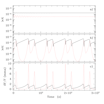
The equilibrium state is a stable attractor for mode triplets with $|\delta\omega|>\gamma_{d}$, and unstable otherwise (Wersinger et al. nl-wersinger80 (1980), Dziembowski nl-dziem82 (1982)). Figures 1a & 1b illustrate these two types of behaviors. Triplets with unstable equilibria undergo a variety of limit cycles. These share a number of common features. The parent mode’s amplitude remains close to its equilibrium (threshold) value, with slow rises on time scale $\gamma^{-1}_{p}$ followed by precipitous drops on time scale $\gamma^{-1}_{d}$. The daughter modes’ amplitudes stay far below their equilibrium values for most of the cycle, but peak with amplitudes comparable to that of the parent mode for a brief interval of length $\gamma^{-1}_{d}$ shortly after the parent mode amplitude reaches its maximum value. During this brief interval, the energy which the parent mode has slowly accumulated is transferred to and dissipated by the daughter modes. So we see that, independent of its stability, the equilibrium state defines the parent mode’s amplitude. This is confirmed by Figure 2a. We employ this result in §3 where we predict upper limits for g-mode amplitudes in pulsating white dwarfs. The time-averaged energies of the daughter modes are also found to be consistent with equations (6)-(7) (Fig. 2b).

3. CHOOSING THE BEST DAUGHTER PAIRS

The discussion in the previous section shows that an overstable parent mode’s amplitude saturates at a value close to the threshold for parametric instability. Although each overstable parent mode has many potential daughter pairs, the most important pair is the one with the lowest instability threshold. This section is devoted to identifying these optimal daughter pairs, a task which separates into two independent parts, maximization of $\kappa^{2}$ and minimization of $(\delta\omega^{2}+\gamma_{d}^{2})$.

3.1. Three-Mode Coupling Coefficients

The 3-mode coupling coefficient characterizes the lowest order nonlinear interactions among stellar modes. A compact form suitable for adiabatic modes under the Cowling approximation is derived in Kumar & Goldreich (nl-kumar89 (1989));

$$\kappa = -\int d^{3}x{{p}\over 6}\left\{(\Gamma_{1}-1)^{2}(\mbox{\boldmath$\nabla$}\cdot{\mbox{\boldmath$\xi$}})^{3}\right.$$ (9)

$$\left.+3(\Gamma_{1}-1)(\mbox{\boldmath$\nabla$}\cdot{\mbox{\boldmath$\xi$}})\xi^{i}_{;j}\xi^{j}_{;i}+2\xi^{i}_{;j}\xi^{j}_{;k}\xi^{k}_{;i}\right\},$$

where $p$ is the unperturbed pressure, $\Gamma_{1}$ is the adiabatic index, $\xi$ is the Lagrangian displacement, the symbol ‘;’ denotes covariant derivative, and the integration is over the volume of the star. This expression for $\kappa$ is symmetric with respect to the three modes. Note that the displacements enter only through components of their gradients. The present form is not suitable for accurate numerical computation. We derive a more appropriate version in §A.1 (eq. [A15]).

Each eigenmode of a spherical star is characterized by three eigenvalues $n,\ell,m$; $n$ is the number of radial nodes in the radial displacement eigenfunction, $\ell$ is the spherical degree, and $m$ is the azimuthal number. Integration over solid angle enforces the following selection rules on triplets with non-vanishing $\kappa$: $|{\ell}_{d_{2}}-{\ell}_{d_{1}}|\leq{\ell}_{p}\leq{\ell}_{d_{1}}+{\ell}_{d_{2}}$, ${\ell}_{p}+{\ell}_{d_{1}}+{\ell}_{d_{2}}$ even, and $m_{p}=m_{d_{1}}+m_{d_{2}}$ (see §A.1). These selection rules guarantee the conservation of angular momentum during nonlinear interactions. The magnitude of $\kappa$ is largest when the eigenfunctions of the daughter modes are radially similar in the upper evanescent zone of the parent mode. Radial similarity requires near equality of the vertical components of WKB wavevectors, $k_{z}$, where for gravity modes $k_{z}^{2}\approx(N^{2}/\omega^{2}-1)\Lambda^{2}/r^{2}$ (eq. [A2] of Paper I) with $N^{2}$ being the Brunt-Väisälä   frequency, $r$ the radius, and $\Lambda^{2}=\ell(\ell+1)$. We take $N\sim\omega_{p}$ as the major contribution to the peak value of $|\kappa|$ comes from the region just above $z_{\omega_{p}}$, the upper boundary of the parent mode’s propagating cavity. The g-mode dispersion relation applicable for $\omega\ll 10^{-2}\,\rm s^{-1}$ is $\omega\propto\ell/n$ (see Fig. 4 of Paper I). We find that $\kappa$ is largest when

$${{n_{d_{1}}}\over{n_{d_{2}}}}\sim{{\Lambda_{d_{1}}\omega_{d_{1}}}\over{\Lambda_{d_{2}}\omega_{d_{2}}}}\sim\left({{\omega_{p}^{2}-\omega_{d_{1}}^{2}}\over{\omega_{p}^{2}-\omega_{d_{2}}^{2}}}\right)^{1/2}.$$ (10)

Taking $\ell_{p}=1$, $\ell_{d_{2}}=\ell_{d_{1}}+1$, and evaluating the above relation for $\ell_{d_{1}}<10$, we locate the peak of $\kappa$ to be at

$$n_{d_{1}}-n_{d_{2}}\approx-0.7n_{p}.$$ (11)

Since a fraction $n_{p}^{-1}$ of the nodes of each daughter mode lie in the region above $z_{\omega_{p}}$, the peak has a width of order $n_{p}$ when measured in $n_{d_{1}}-n_{d_{2}}$. Figure 3 illustrates the behavior of $\kappa$ for a variety of combinations of parent and daughter modes.

Figure 3.— Coupling coefficient $\kappa$ in ${\rm erg}^{-1/2}$ for a DA white dwarf model with $T_{\rm eff}=12,800\,\rm K$. From top to bottom panels, we consider four ${\ell_{p}}=1$ parent modes with increasing $n_{p}$. Coupling coefficients between each parent and its daughter pairs are plotted versus $n_{d_{1}}-n_{d_{2}}$. Solid lines denote daughter pairs with ${\ell_{d_{1}}}=1$, and others those with ${\ell_{d_{1}}}=2,3,4,5$, and $9$. Mode $3$ is chosen to minimize $|\delta\omega|$ subject to the constraint ${\ell}_{d_{2}}={\ell}_{p}+{\ell}_{d_{1}}$. $\kappa$ is seen to depend on the radial similarity of the two daughter modes (eq. [10]) but not on their spherical degrees. The FWHM of the peak in $|\kappa|$ is of order $n_{p}$. Maximum $|\kappa|$ occurs for $n_{d_{1}}-n_{d_{2}}\sim-0.7n_{p}$ (eq. [11]).

Figure 4.— Coupling coefficients as a function of parent mode’s radial order. We consider $\ell_{p}=1$ parent modes, and include all daughter pairs that have ${\ell}_{d_{1}}={1,...,9}$ and ${\ell}_{d_{2}}={\ell}_{p}+{\ell}_{d_{1}}$. For each mode $2$, mode $3$ is chosen to minimize $|\delta\omega|$. The solid line corresponds to the theoretical estimate for the maximum $|\kappa|$ at each $n_{p}$ (eq. [12]). $L$ is the stellar luminosity, and $\tau_{\omega_{p}}$ is the thermal time at $z_{\omega_{p}}$. These calculations are based on the same stellar model used for Figure 3.

As we show in §A.2, the maximum value of $|\kappa|$ is of order

$$|\kappa|_{\rm max}\sim\frac{1}{\left(n_{p}^{3}\tau_{\omega_{p}}L\right)^{1/2}}.$$ (12)

Here $L$ is the stellar luminosity and $\tau_{\omega_{p}}$ is the thermal timescale at $z_{\omega_{p}}$. This is compared with numerical results in Figure 4. Note that the maximum value of $\kappa$ depends entirely upon the properties of the parent mode and not at all upon those of its daughters.

3.2. Frequency Mismatch and Damping Rates

Because the maximum value of $|\kappa|$ is independent of $\ell_{d_{1}}$ and $\ell_{d_{2}}$, we choose these parameters to minimize $(\delta\omega^{2}+\gamma_{d}^{2})$.

Consider an $\ell_{p},m_{p}$ parent mode. For each choice of $\ell_{d_{1}},\ell_{d_{2}}$, there are of order $\ell_{d_{1}}n_{p}^{2}$ daughter pairs for which $\kappa$ is close to its maximum value. The factor $\ell_{d_{1}}$ arises from the freedom in choosing $m_{d_{1}}$, while the factor $n_{p}^{2}$ comes from the width of maximum $|\kappa|$ at each $\ell_{d_{1}}$. Relaxing the value of $\ell_{d_{2}}$ subject to the constraint of the angular selection rules increases the number of pairs by a factor of order $\ell_{p}$. Now replace $\ell_{d_{1}}$ by a running variable ${\ell_{d_{1}}}^{\prime}$. The number of pairs with ${\ell_{d_{1}}}^{\prime}\leq\ell_{d_{1}}$ is of order $\ell_{p}\ell_{d_{1}}^{2}n_{p}^{2}$. The distribution of the $\delta\omega$ values of these pairs is uniform between $0$ and $n_{p}\omega_{d_{1}}/n_{d_{1}}$. Statistically, the minimum frequency mismatch

$$\Delta\omega\sim{{\omega_{d_{1}}}\over{n_{d_{1}}}}{1\over{\ell_{p}\ell_{d_{1}}^{2}n_{p}}}\sim{{\omega_{p}}\over{\ell_{d_{1}}^{3}n_{p}^{2}}},$$ (13)

where the low frequency limit of the dispersion relation, $\omega\propto\ell/n$, is assumed in going from the first to the second relation for $\Delta\omega$. Our estimate for $\Delta\omega$ assumes that rotation lifts $m$ degeneracy. If it does not, the minimum frequency mismatch is increased by a factor of $\ell_{d_{1}}$.

Figure 5.— Nonadiabatic energy driving and damping rates as a function of mode period. See Paper II for computational details. We consider three stellar models with decreasing effective temperature; $\tau_{\rm th}$ is the thermal time scale at the bottom of the convective zone. Overstable modes are marked by solid triangles. Lines connect points associated with modes of the same $\ell$. For each $\ell$, $\gamma$ exhibits an initial steep rise with increasing mode period (eq. [14]), followed by a gradual decline (eq. [15]). Maximum $\gamma$ occurs at the transition between quasi-adiabatic and strongly nonadiabatic damping.

Next we describe how $\gamma$ varies with $\omega$ and $\ell$. There are two regimes of relevance to this investigation. In the quasiadiabatic limit (cf. §4.4 of paper I),

$$\gamma\sim{1\over{n\tau_{\omega}}}\propto\left({\ell\over\omega}\right)^{6}.$$ (14)

In the strongly nonadiabatic limit (see §B.1),

$$\gamma\sim{\omega\over{\pi n}}\ln{1\over{\cal R}}\propto\omega^{0.75}\ell^{0.2},$$ (15)

where ${\cal R}$ is the amplitude reflection coefficient at the top of the mode’s cavity. The transition between the quasiadiabatic and strongly nonadiabatic limits is marked by a significant reduction of ${\cal R}$ by radiative diffusion. The behavior of $\gamma$ as a function of $\omega$ and $\ell$ is illustrated in Figure 5. Radial similarity of the daughter modes to which a given parent mode couples most strongly (eq.[10]) implies $\gamma_{d_{1}}\approx\gamma_{d_{2}}\approx\gamma_{d}$.

Figure 6.— Selection of the best daughter pairs for a few low order $\ell_{p}=1$ parent modes in a white dwarf model with $T_{\rm eff}=12,800\,\rm K$. We look at daughter pairs with $\ell_{d_{1}}$ ranging from $1$ to $100$, and $\ell_{d_{2}}=\ell_{d_{1}}+\ell_{p}$. We plot $(\gamma_{d_{1}}\gamma_{d_{2}})^{1/2}$ in the upper panel, and $|\delta\omega|$ in the middle panel, for the pair that sets the lowest instability threshold at each $\ell_{d_{1}}$. This does not necessarily correspond to the pair that give rise to the lowest $|\delta\omega|$ at each $\ell_{d_{1}}$. The corresponding threshold value of $(\delta p/p)_{p}$ evaluated at the stellar surface is shown in the bottom panel. With increasing $\ell_{d_{1}}$, $(\gamma_{d_{1}}\gamma_{d_{2}})^{1/2}$ rises and $|\delta\omega|$ becomes unimportant. The best daughter pairs have low $\ell$ values.

The minimum of $(\delta\omega^{2}+\gamma_{d}^{2})$ is attained for daughter pairs that satisfy $\delta\omega^{2}\lesssim\gamma_{d}^{2}$. With increasing $n_{p}$, the value of $\ell_{d_{1}}$ at which this occurs decreases from a few to unity (see Fig. 6). For sufficiently large values of $n_{p}$, $\Delta\omega\ll\gamma_{d}$ even for $\ell_{d_{1}}=1$.

4. UPPER ENVELOPE OF PARENT MODE AMPLITUDES

Parametric instability provides an upper envelope to the amplitudes of overstable modes. Coupling of an overstable parent mode to a single pair of daughter modes suffices to maintain the parent mode’s amplitude near the threshold value (cf. §2.2). The energy gained by the overstable parent mode and transferred to the daughter modes may be disposed of by linear radiative damping or by further nonlinear coupling to granddaughter modes.

The results presented in this section are obtained from numerical computations and displayed in a series of figures. The general trends they exhibit are best understood in terms of analytic scaling relations. We derive these first in order to be able to refer to them as we describe each figure.

Excited modes of ZZ Ceti stars are usually detected through photometric measurements of flux variations, and in a few cases through spectroscopic measurements of horizontal velocity variations. Hence we calculate surface amplitudes of fractional flux, $\Delta F/F$, and horizontal velocity, $v_{h}$, variations. Each of these is directly related to the near surface amplitude of the Lagrangian pressure perturbation, $\delta p/p$. The threshold value of the latter is obtained by combining equations (4) and (12) with the normalization factor $(n\tau_{\omega}L)^{-1/2}$ given by equation (A28) of Paper I. Thus

$${\delta p\over p}\sim n\left[\left({\gamma_{d}\over\omega}\right)^{2}+\left({\delta\omega\over\omega}\right)^{2}\right]^{1/2}.$$ (16)

Adopting relations expressing $v_{h}$ and $\Delta F/F$ in terms of $\delta p/p$ from §3 of Paper I, we arrive at

$$v_{h}\approx{\omega Rn\over[\ell(\ell+1)]^{1/2}}\left[\left({\gamma_{d}\over\omega}\right)^{2}+\left({\delta\omega\over\omega}\right)^{2}\right]^{1/2},$$ (17)

and

$${\Delta F\over F}\approx{n\over\left[1+\left(\omega\tau_{c}\right)^{2}\right]^{1/2}}\left[\left({\gamma_{d}\over\omega}\right)^{2}+\left({\delta\omega\over\omega}\right)^{2}\right]^{1/2},$$ (18)

In the above, $R$ denotes the stellar radius, and $\tau_{c}$ is the thermal time constant describing the low pass filtering action of the convection zone on flux variations input at its base.

Figure 7.— An assembly of results on threshold amplitudes for parametric instability. From left to right, amplitudes of overstable modes with different $\ell$ are plotted against mode period. From top to bottom, the panels display photospheric amplitudes of fractional pressure perturbation, horizontal velocity, and fractional flux variation. Filled circles, crosses, and open squares symbolize modes from the three stellar models in Figure 5 in order of descending $T_{\rm eff}$. Pulsation amplitudes generally rise with increasing mode period, except for the shortest period modes which exhibit large star to star fluctuations. Amplitudes of $|\delta p/p|$ for $\ell=1$ modes in the coolest model dip around $600\,\rm s$ and flatten beyond $1200\,\rm s$. The first feature is associated with the dip in $\gamma$ for neutrally stable daughter modes, and the second is explained by the flattening of $\gamma$ for strongly nonadiabatic daughter modes of long period (see Fig. 5). Reduction of the coupling coefficient due to strong nonadiabaticity is not accounted for (see appendix B.2).

Figure 7 displays calculated values for amplitudes of overstable modes limited by parametric instability. The rise of $|\delta p/p|$ with increasing mode period mainly reflects the corresponding rise of the damping rates of the daughter modes (cf. §3.2) as indicated by equation (16). At the longer periods, the values of $|\delta p/p|$ decline with decreasing $T_{\rm eff}$. This is a subtle consequence of the deepening of the convection zone which pushes down the top of the daughter modes’ cavities, thus reducing their damping rates (see §5.2 of Wu & Goldreich nl-paperII (1999), hereafter Paper II). The behavior of $|v_{h}|$ is similar to that of $|\delta p/p|$ except that $|v_{h}|$ decreases relative to $|\delta p/p|$ with increasing $\ell$ as shown by comparison of equations (16) and (17). A new feature present in the run of $|\delta F/F|$ verses mode period is the low pass filtering action of the convection zone as expressed by the factor $[1+(\omega\tau_{c})^{2}]^{-1/2}$ in equation (18). This factor causes $|\delta F/F|$ to rise slightly more steeply than $|\delta p/p|$ with increasing mode period. It is also responsible for a more dramatic decrease in $|\delta F/F|$ with decreasing $T_{\rm eff}$ at fixed mode period. Since $|v_{h}|$ does not suffer from this visibility reduction, velocity variations may be observable in stars that are cooler than those at the red edge of the instability strip.

Figure 8.— Comparison between theoretical parametric amplitudes and those summarized by Clemens (amp-clemens93 (1993)) from observations of two dozen DA variables. Each star is represented by a filled circle plotted such that the ordinate gives the photometric amplitude of the largest mode and the abscissa the mean period weighted by the photometric amplitudes of all its detected modes. To compare theory and observation, we single out the largest amplitude $\ell=1$ mode for each of the three models used in Figure 7. The solid line is an interpolation between these largest amplitude modes and their periods. The amplitudes are reduced by a factor of $2.5$ to approximately account for the reduction in visible relative to bolometric flux variations for DA variables. The run of observed mode amplitude as a function of mode period is mimicked by the solid line. However, the extrapolation to short period shown by the dotted line is not reliable, because in this regime mode amplitudes have large star-to-star variations associated with different values of frequency mismatches. The drop-off in amplitude at long period ($P>10^{3}\,\rm s$) results from a combination of lower daughter mode damping rates and a reduction in the visibility of the parent mode due to increasing $\omega\tau_{c}$. Turbulent dissipation arising from the shear layer below the convection zone (§5.1) further suppresses the amplitudes that long period modes can attain. This is illustrated by the dashed curves for different choices of the drag coefficient, $C_{D}$.

Figure 9.— Energy versus period for overstable modes in the coolest model considered in Figure 7. Solid, dashed and dotted lines represent $\ell=1$, $2$ and $3$ modes. Mode energy tends to decrease with increasing period and with increasing $\ell$. Deviations from this trend for the $\ell=1$ modes are explained as follows. The narrow dip near $200\,\rm s$ is due to a fortuitiously good frequency resonance involving the $n=2$ mode, and the wider dip around $700\,\rm s$ is associated with neutrally stable daughter modes.

Figure 8 reproduces a summary of observational data on mode amplitudes from Clemens (amp-clemens95 (1995)). Each star is represented by a point showing the relation between the V-band photometric amplitude in its largest mode and the amplitude weighted mean period of all its observed modes. The latter quantity is a surrogate for the star’s effective temperature in the sense that longer mean periods correspond to lower effective temperatures (Clemens amp-clemens95 (1995), Paper I). Our theoretical predictions for the amplitudes of $\ell=1$ modes limited by parametric instability are shown by a solid line obtained by interpolation from the numerical results displayed in Figure 7. Two features of this figure are worthy of comment.

For a few low order overstable modes, $n_{p}\leq 3$ at $\ell_{p}=1$, $\delta\omega$ is more significant than $\gamma_{d}$ in determining the best daughter pair (Fig. 6). The best daughter pairs for these modes have $\ell$ values of a few and identities which depend sensitively on minor differences among stars. Thus we expect amplitudes of short period overstable modes to show large star to star variations. That the $n=1,\ell=1$ mode is detected in only about one half of the hot DAVs (see Figure 4 of Clemens amp-clemens95 (1995)) is consistent with the expected statistical variations in $\delta\omega$.

Overstable $\ell=1$ modes with periods longer than $800\,\rm s$ ($n_{p}\geq 20$) are probably not saturated by parametric instability. Their maximum $|\kappa|$ is severely reduced below the adiabatic value by the strong nonadiabaticity of their daughter modes (§B.2). Other mechanisms that contribute towards saturating these modes are discussed in §5.

5. DISCUSSION

5.1. Turbulent Saturation

Turbulent convection severely reduces the vertical gradient of the horizontal velocity of g-modes in the convection zone. As a result, a shear layer forms at the boundary between the bottom of the convection zone and the top of the radiative interior (Goldreich & Wu nl-paperIII (1999), hereafter Paper III). Kelvin-Helmholtz instability of this layer provides a nonlinear dissipation mechanism for overstable modes. An overstable mode’s amplitude cannot grow beyond the value at which nonlinear damping due to the Kelvin-Helmholtz instability balances its linear convective driving. Equation (44) of Paper III provides an estimate for the value at which this mechanism saturates the surface amplitude of $(\delta p/p)$;

$$\left({\delta p\over p}\right)\sim{0.1\over C_{D}}{[(\omega\tau_{c})^{2}+1]^{1/2}[(\omega\tau_{c})^{2}-1]\over\omega\tau_{c}}{Lz_{\omega}^{2}\over Rz_{b}}.$$ (19)

Our ignorance of the complicated physics involved in a nonlinear shear layer is covered by the range of possible values of the dimensionless drag coefficient, $C_{D}$. Terrestrial experiments indicate that $C_{D}$ falls between $10^{-3}$ and $10^{-1}$. The dashed lines in Figure 8 show the effect of including nonlinear turbulent damping in addition to parametric instability on limiting mode amplitudes. Amplitudes of overstable modes saturated by the Kelvin-Helmholtz instability are uncertain because $C_{D}$ is poorly constrained.

5.2. Granddaughter Modes

Here we answer the following questions. Under what conditions do daughter modes excite granddaughter modes by parametric instability? What are the consequences if they do? In §2.2 we show how parametric instability of linearly damped daughter modes maintains the amplitude of a parent mode close to its equilibrium value. In order to dispose of the energy they receive from the parent mode, the time averaged energies of the daughter modes must be close to their equilibrium values. This raises a worry. Suppose the daughters are prevented from reaching their equilibrium amplitudes by parametric instability of granddaughter modes Then they would not be able to halt the amplitude growth of the parent mode.

To answer the first of these questions, we calculate the ratio, denoted by the symbol ${\cal S}$, between the threshold amplitude for a daughter mode to excite granddaughter modes and its equilibrium amplitude under parametric excitation by the parent mode. The former is obtained from equation (4), and the latter from equations (6)-(7). We make a few simplifying assumptions to streamline the discussion. Resonances between daughters and granddaughters are taken as exact; individual members of daughter and granddaughter pairs are treated as equivalent. Equations (12) and (14) are combined to yield

$$\kappa^{2}\sim\frac{\gamma_{p}}{n_{p}^{2}L}.$$ (20)

It is then straightforward to show that

$${\cal S}\approx\frac{\omega_{p}\omega_{d}}{\omega_{g}^{2}}\left(\frac{n_{d}}{n_{p}}\right)^{2}\left(\frac{\gamma_{g}^{2}}{\gamma_{d}^{2}+\delta\omega^{2}}\right)\approx 32\left(\frac{\gamma_{g}^{2}}{\gamma_{d}^{2}+\delta\omega^{2}}\right).$$ (21)

The factor $32$ is an approximation based on taking $\omega_{g}/\omega_{d}=\omega_{d}/\omega_{p}=1/2$ and $n_{p}/n_{d}=1/2$.

In general ${\cal S}\gg 1$, so the excitation of granddaughter modes requires the daughter modes to have energies in excess of their equilibrium values. However, the equilibrium solution is unstable if the best daughter pair corresponds to $\gamma_{d}>|\delta\omega|$, and then the daughter mode energies episodically rise far above their equilibrium values. At such times, granddaughter modes may be excited by parametric instability and consequentially limit the amplitude growth of the daughter modes. This slows the transfer of energy from parent to daughter modes, but it does not prevent the daughter modes from saturating the growth of the parent mode’s amplitude at the level described by equation (4).

For the few lowest order parent modes, we typically find $|\delta\omega|\geq\gamma_{d}$. This may reduce ${\cal S}$ to below unity with the consequence that the parent mode amplitude may rise above that given by equation (4).

5.3. Additional 3-Mode Interactions

Parametric instability sets reasonable upper bounds on the photospheric amplitudes of overstable modes. In a given star this upper bound rises with increasing mode period except possibly for the lowest few modes. However, the observed amplitude distributions are highly irregular. This mode selectivity may arise from 3-mode interactions which involve more than one overstable mode.

We investigate a particular example of this type. It is closely related to parametric instability, the only difference being that the daughter modes of the overstable parent mode are themselves overstable. Acting in isolation, resonant mode couplings tend to drive mode energies toward equipartition. They conserve the total energy, ${\dot{E}}_{p}+{\dot{E}}_{d_{1}}+{\dot{E}}_{d_{2}}=0$, and transfer action according to ${\dot{E}}_{d_{1}}/\omega_{d_{1}}={\dot{E}}_{d_{2}}/\omega_{d_{2}}=-{\dot{E}}_{p}/\omega_{p}$. In this context it is important to note that the energies of overstable modes limited by parametric instability decline with increasing mode period (Fig. 9). Therefore nonlinear interactions transfer energy from the parent mode to its independently excited daughters. As shown below, this transfer may severely suppress the parent mode’s amplitude.

We start from equations (1)-(3). These may be manipulated to yield

$${dE_{p}\over dt}=\gamma_{p}E_{p}+3\sqrt{2}\omega_{p}\kappa(E_{p}E_{d_{1}}E_{d_{2}})^{1/2}\sin\Phi,$$ (22)

where $\Phi=\theta_{d_{1}}+\theta_{d_{2}}-\theta_{p}$. For $E_{p}\gg E_{d_{1}}$ and $E_{d_{2}}$, nonlinear interactions transfer energy from the parent mode to its daughter modes. In particular, if we ignore phase changes in the overstable daughter modes due to their interactions with granddaughter modes, we find that $\Phi$ satisfies

$$\frac{d\Phi}{dt}=\delta\omega-\frac{3}{\sqrt{2}}\kappa(E_{p}E_{d_{1}}E_{d_{2}})^{1/2}\left[\left(\frac{\omega_{d_{1}}}{E_{d_{1}}}+\frac{\omega_{d_{2}}}{E_{d_{2}}}\right)-\frac{\omega_{p}}{E_{p}}\right]\cos\Phi,$$ (23)

with a stable solution at $\Phi=-\pi/2$ when $\delta\omega=0$.

We denote the ratio of the nonlinear term to the linear term in equation (22) by the symbol ${\cal T}$;

$${\cal T}\approx\frac{3\sqrt{2}\omega_{p}\kappa}{\gamma_{p}}\left(\frac{E_{d_{1}}E_{d_{2}}}{E_{p}}\right)^{1/2}.$$ (24)

Using the magnitudes of $E_{i}$ set by parametric instability of their respective daughters, and adopting the same approximations made in §5.2, we arrive at

$${\cal T}\approx\frac{\omega_{p}\omega_{d}}{\omega_{g}^{2}}\left(\frac{n_{d}}{n_{p}}\right)^{2}\left(\frac{\gamma_{g}^{2}}{\gamma_{d}^{2}+\delta\omega^{2}}\right)\approx 32\left(\frac{\gamma_{g}^{2}}{\gamma_{d}^{2}+\delta\omega^{2}}\right).$$ (25)

Comparing equations (21) and (25) we see that ${\cal S=T}$. A little thought reveals that this is not a coincidence. For ${\cal T}\gg 1$, overstable daughter modes can suppress a parent mode’s energy below the value set by parametric instability. We expect this suppression to be important in cool ZZ Ceti stars whose overstable modes extend to long periods. It may render their intermediate period modes invisible. In a similar manner, the amplitudes of high frequency overstable modes with $\ell=2$ and $3$ may be heavily suppressed by interactions with their lowest $\ell$ overstable daughters.

The irregular amplitude distributions among neighboring modes may be partially accounted for by this type of resonance. Mode variability may also play a role. We explore this in the next subsection.

5.4. Mode Variability

Excited g-modes in ZZ Ceti stars exhibit substantial temporal variations. Parametric instability may at least partially account for these variations.

When $|\delta\omega|<\gamma_{d}$, parametric instability gives rise to limit cycles in which the amplitudes and phases of parent and daughter modes vary on time scales as short as $\gamma^{-1}_{d}$. Stable daughter modes may briefly attain visible amplitudes. Temporal amplitude variations may contribute to the irregular mode amplitude distribution seen in individual stars.

Phase variations of a parent mode obey the equation

$${{d\theta_{p}}\over{dt}}=\omega_{p}-{3\over{\sqrt{2}}}\omega_{p}\kappa{{|A_{d_{1}}||A_{d_{2}}|}\over{|A_{p}|}}\cos\Phi.$$ (26)

At the equilibrium given by equations (5)-(8), the parent mode’s frequency is displaced from its unperturbed value such that

$$\omega_{p}^{\prime}={{d\theta_{p}}\over{dt}}=\omega_{p}+{{\delta\omega\gamma_{p}}\over{\gamma_{d_{1}}+\gamma_{d_{2}}-\gamma_{p}}}\sqrt{1+\left({{2\delta\omega}\over{\gamma_{d_{1}}+\gamma_{d_{2}}-\gamma_{p}}}\right)^{2}}.$$ (27)

This constant frequency shift is of order $10^{-9}s^{-1}$ for the $n=1$, $\ell=1$ mode and of order $10^{-7}s^{-1}$ for the $n=2$, $\ell=2$ mode. Frequency shifts in higher order overstable modes which are involved in limit cycles are predicted to be larger and time variable. During brief intervals of length $\sim\gamma^{-1}_{d}$, when the daughter mode energies are comparable to that of the parent mode, $|\omega_{p}^{\prime}-\omega_{p}|\sim\gamma_{d}$, which is of order a few times $10^{-5}s^{-1}$, or a few $\mu Hz$ in angular frequency. These shifts might account for the time-varying rotational splittings reported by Kleinman et al. (kleinmanZZPsc (1998)) provided different $m$ components of the overstable modes are involved in different limit cycles.

5.5. Miscellany

We briefly comment on two relevant issues.

Gravitational settling produces chemically pure layers between which modes can be partially trapped. Modes that are trapped in the hydrogen layer have lower mode masses, and therefore higher growth rates and larger maximum values of $|\kappa|$ than untrapped modes of similar frequency. This implies lower threshold energies for parametric instability. Nevertheless, trapping does not affect predicted photospheric amplitudes of $\delta p/p$, and hence $v_{h}$ and $\delta F/F$, since these are proportional to $A$ divided by the square root of the mode mass.

In circumstances of small rotational splitting, the simple limit-cycles depicted in Figure 1 are unlikely to be realistic. In such cases, different $m$ components of an overstable parent mode share some common daughter modes. This leads to more complex dynamics.

Appendix A Three-Mode Coupling Coefficient

We reproduce the expression for the three-mode coupling coefficient presented in equation (9) of §3.1 with one modification:

$$\kappa=-\int d^{3}xp\left\{{{\Gamma_{1}(\Gamma_{1}-2)}\over 6}(\mbox{\boldmath$\nabla$}\cdot{\mbox{\boldmath$\xi$}})^{3}+{1\over 2}\Gamma_{1}(\mbox{\boldmath$\nabla$}\cdot{\mbox{\boldmath$\xi$}})\xi^{i}_{;j}\xi^{j}_{;i}+{\rm Det}|\xi^{i}_{;j}|\right\},$$ (A1)

where

$${\rm Det}|\xi^{i}_{;j}|={1\over 6}(\mbox{\boldmath$\nabla$}\cdot{\mbox{\boldmath$\xi$}})^{3}-{1\over 2}(\mbox{\boldmath$\nabla$}\cdot{\mbox{\boldmath$\xi$}})\xi^{i}_{;j}\xi^{j}_{;i}+{1\over 3}\xi^{i}_{;j}\xi^{j}_{;k}\xi^{k}_{;i}.$$ (A2)

Because of strong cancellations among its largest terms, this form is not well-suited for numerical evaluation. We derive a new expression which does not suffer from this defect. Then we estimate the size of $\kappa$ and deduce its dependences upon the properties of the three-modes.

A.1. Simplification

In spherical coordinates $(r,\theta,\phi)$, the components of the displacement vector may be written as

$${\mbox{\boldmath$\xi$}}=\xi^{i}\mbox{\boldmath$\varepsilon$}_{i}=\left[\xi_{r}(r),{{\xi_{h}(r)}\over r}{\partial\over{\partial\theta}},{{\xi_{h}(r)}\over r}{1\over{\sin^{2}{\theta}}}{\partial\over{\partial\phi}}\right]Y_{{\ell}m}(\theta,\phi),$$ (A3)

where $Y_{\ell m}$ is a spherical harmonic function, and the $\mbox{\boldmath$\varepsilon$}_{i}$ are covariant basis vectors.

The angular integrations in equation (A1) are done analytically. The following definitions and properties prove useful:

$$T \equiv \int_{0}^{2\pi}d\phi\int_{0}^{\pi}d\theta\,\sin\theta Y_{a}Y_{b}Y_{c}\equiv<Y_{a}Y_{b}Y_{c}>,$$ (A4a)

$$F_{a} \equiv <Y_{a}\nabla_{\alpha}Y_{b}\nabla^{\alpha}Y_{c}>=\left(\Lambda_{b}^{2}+\Lambda_{c}^{2}-\Lambda_{a}^{2}\right){T\over 2},$$ (A4b)

$$G_{a} \equiv <\nabla_{\alpha}\nabla_{\beta}Y_{a}\nabla^{\alpha}Y_{b}\nabla^{\beta}Y_{c}>\equiv\left[\Lambda_{a}^{4}-(\Lambda_{b}^{2}-\Lambda_{c}^{2})^{2}\right]{T\over 4},$$ (A4c)

$$S \equiv <\nabla_{\alpha}(\nabla^{\alpha}Y_{a}\nabla_{\beta}Y_{b}\nabla^{\beta}Y_{c})>=G_{a}+G_{b}+G_{c}$$ (A4d)

$$= {1\over 2}(\Lambda_{a}^{2}F_{a}+\Lambda_{b}^{2}F_{b}+\Lambda_{c}^{2}F_{c})=G_{a}+\Lambda_{a}^{2}F_{a},$$

$$V_{a} \equiv <Y_{a}\nabla_{\alpha}\nabla^{\beta}Y_{b}\nabla_{\beta}\nabla^{\alpha}Y_{c}>=\Lambda_{b}^{2}\Lambda_{c}^{2}T-F_{a}-S,$$ (A4e)

$$\Lambda_{a}^{2}T = F_{b}+F_{c},$$ (A4f)

$$\Lambda_{a}^{2}F_{a} = G_{b}+G_{c}.$$ (A4g)

Here, $\nabla_{\alpha}$ is the covariant derivative on a spherical surface; $\alpha$ can be either $\theta$ or $\phi$. Each angular integration is proportional to $T$ which contains all $m$ dependences and is of order unity independent of the $\ell$ values of the participating modes. The paramter $\Lambda^{2}\equiv\ell(\ell+1)$. Subscripts $a$, $b$ and $c$ denote different modes. The angular selection rules are simply, ${\ell}_{c}\in[|{\ell}_{a}-{\ell}_{b}|,{\ell}_{a}+{\ell}_{b}]$, Mod$[({\ell}_{c}+{\ell}_{b}+{\ell}_{c}),2]=0$ and $m_{a}+m_{b}+m_{c}=0$.

Angular integration of ${\rm Det}|\xi^{i}_{;j}|$ yields

$$\oint d\Omega\,{\rm Det}|\xi^{i}_{;j}| = {1\over r^{2}}\left[T\xi^{b}_{r}\xi^{c}_{r}-\Lambda_{c}^{2}T\xi^{b}_{r}\xi^{c}_{h}+{1\over 2}{(\Lambda_{b}^{2}\Lambda_{c}^{2}T-V_{a})}\xi^{b}_{h}\xi^{c}_{h}\right]{{d\xi^{a}_{r}}\over{dr}}$$ (A5)

$$+{1\over r^{2}}\left[S(\xi^{b}_{r}-\xi^{b}_{h})\xi^{c}_{h}-F_{b}\xi^{b}_{r}(\xi^{c}_{r}-\xi^{c}_{h})\right]{{d\xi^{a}_{h}}\over{dr}}.$$

Symmetrizing this expression with respect to modes $b$ and $c$, employing equations (A4d)-(A4g), we get

$$\oint d\Omega\,{\rm Det}|\xi^{i}_{;j}|=-{S\over{3r^{2}}}{d\over{dr}}\left(\xi^{a}_{h}\xi^{b}_{h}\xi^{c}_{h}\right)+{{(F_{a}+S)}\over{2r^{2}}}{d\over{dr}}\left(\xi^{a}_{r}\xi^{b}_{h}\xi^{c}_{h}\right)-{{\Lambda_{a}^{2}T}\over{2r^{2}}}{d\over{dr}}\left(\xi^{a}_{h}\xi^{b}_{r}\xi^{c}_{r}\right)+{T\over{3r^{2}}}{d\over{dr}}\left(\xi^{a}_{r}\xi^{b}_{r}\xi^{c}_{r}\right).$$ (A6)

For gravity-modes, $|\xi_{h}|\gg|\xi_{r}|$. Thus the four terms in this expression decrease in size from left to right.

In a similar manner we arrive at

$$\oint d\Omega\,(\mbox{\boldmath$\nabla$}\cdot{\mbox{\boldmath$\xi$}})^{3}=T(\mbox{\boldmath$\nabla$}\cdot{\mbox{\boldmath$\xi$}}^{a})(\mbox{\boldmath$\nabla$}\cdot{\mbox{\boldmath$\xi$}}^{b})(\mbox{\boldmath$\nabla$}\cdot{\mbox{\boldmath$\xi$}}^{c}),$$ (A7)

and

$$\oint d\Omega\,(\mbox{\boldmath$\nabla$}\cdot{\mbox{\boldmath$\xi$}})\xi^{i}_{;j}\xi^{j}_{;i} = -{{F_{a}}\over r}(\mbox{\boldmath$\nabla$}\cdot{\mbox{\boldmath$\xi$}}^{a}){d\over{dr}}\left(\xi^{b}_{h}\xi^{c}_{h}\right)+{{2F_{a}}\over r}(\mbox{\boldmath$\nabla$}\cdot{\mbox{\boldmath$\xi$}}^{a})\xi^{b}_{r}{{d\xi^{c}_{h}}\over{dr}}+T(\mbox{\boldmath$\nabla$}\cdot{\mbox{\boldmath$\xi$}}^{a}){{d\xi^{b}_{r}}\over{dr}}{{d\xi^{c}_{r}}\over{dr}}$$ (A8)

$$+{{V_{a}}\over{r^{2}}}(\mbox{\boldmath$\nabla$}\cdot{\mbox{\boldmath$\xi$}}^{a})\xi^{b}_{h}\xi^{c}_{h}-{{2T\Lambda_{c}^{2}}\over{r^{2}}}(\mbox{\boldmath$\nabla$}\cdot{\mbox{\boldmath$\xi$}}^{a})\xi^{b}_{r}\xi^{c}_{h}+{{2T}\over{r^{2}}}(\mbox{\boldmath$\nabla$}\cdot{\mbox{\boldmath$\xi$}}^{a})\xi^{b}_{r}\xi^{c}_{r}.$$

The magnitudes of the terms in the above expression decrease from left to right except that terms 2-4 are of comparable size.

Having disposed of the angular dependences in $\kappa$, we turn to the radial integrations. The following relations prove helpful in this context:

$${{d\xi_{r}}\over{dr}} = (\mbox{\boldmath$\nabla$}\cdot{\mbox{\boldmath$\xi$}})+{{\Lambda^{2}}\over r}\xi_{h}-{2\over r}\xi_{r},$$ (A9)

$${d\over{dr}}\left[\Gamma_{1}p(\mbox{\boldmath$\nabla$}\cdot{\mbox{\boldmath$\xi$}})\right] = {{\Lambda^{2}\rho g}\over r}\xi_{h}-\left(\omega^{2}+{{2g}\over r}-{{dg}\over{dr}}\right)\rho\xi_{r},$$ (A10)

$$\Gamma_{1}p(\mbox{\boldmath$\nabla$}\cdot{\mbox{\boldmath$\xi$}}) = \rho g\xi_{r}-r\rho\omega^{2}\xi_{h}.$$ (A11)

The first equation is the definition of divergence, and the second and third are the radial and horizontal components of the equation of motion written in terms of the Lagrangian displacement.

Curvature terms arise because the directions of the basis vectors depend upon position. For instance,

$$\xi^{r}_{;\theta}=(\xi_{r}-\xi_{h}){{\partial Y_{\ell m}}\over{\partial\theta}},$$ (A12)

where $\xi_{h}$ appears due to curvature in the coordinate system. The largest terms in equations (A6) and (A8) are curvature terms. However, their radial integrals cancel leaving a much smaller net contribution. Direct numerical evaluation of equation (A1) leads to unreliable results, so it is important to carry out this cancellation analytically. Accordingly, we integrate each term by parts and apply equations (A4d) and (A9) to obtain

$$\int_{0}^{R}dr\,\left[{Sp\over 3}{d\over{dr}}\left(\xi^{a}_{h}\xi^{b}_{h}\xi^{c}_{h}\right)+{{F_{a}r\Gamma_{1}p}\over 2}(\mbox{\boldmath$\nabla$}\cdot{\mbox{\boldmath$\xi$}}^{a}){d\over{dr}}\left(\xi^{b}_{h}\xi^{c}_{h}\right)\right]$$

$$=-\int_{0}^{R}dr\,{{F_{a}\Gamma_{1}p}\over 2}(\mbox{\boldmath$\nabla$}\cdot{\mbox{\boldmath$\xi$}}^{a})\xi^{b}_{h}\xi^{c}_{h}+\int_{0}^{R}dr\,{{F_{a}r\rho}\over 2}\left(\omega_{a}^{2}+{{2g}\over r}-{{dg}\over{dr}}\right)\xi^{a}_{r}\xi^{b}_{h}\xi^{c}_{h}.$$ (A13)

This step leads to

$$\kappa = \int_{0}^{R}dr\,\left[-{Tr^{2}{\Gamma_{1}(\Gamma_{1}-2)p}\over{6}}(\mbox{\boldmath$\nabla$}\cdot{\mbox{\boldmath$\xi$}}^{a})(\mbox{\boldmath$\nabla$}\cdot{\mbox{\boldmath$\xi$}}^{b})(\mbox{\boldmath$\nabla$}\cdot{\mbox{\boldmath$\xi$}}^{c})-{Tr^{2}{\Gamma_{1}p}\over 2}(\mbox{\boldmath$\nabla$}\cdot{\mbox{\boldmath$\xi$}}^{a}){{d\xi^{b}_{r}}\over{dr}}{{d\xi^{c}_{r}}\over{dr}}\right.$$ (A14)

$$\left.\hskip-22.76228pt-F_{a}r\Gamma_{1}p(\mbox{\boldmath$\nabla$}\cdot{\mbox{\boldmath$\xi$}}^{a})\xi^{b}_{r}{{d\xi^{c}_{h}}\over{dr}}-{(\Lambda_{b}^{2}\Lambda_{c}^{2}T-S){\Gamma_{1}p}\over{2}}(\mbox{\boldmath$\nabla$}\cdot{\mbox{\boldmath$\xi$}}^{a})\xi^{b}_{h}\xi^{c}_{h}-{{(S-F_{a})\rho g}\over{2}}\xi^{a}_{r}\xi^{b}_{h}\xi^{c}_{h}-{{F_{a}r\rho}\over{2}}{{dg}\over{dr}}\xi^{a}_{r}\xi^{b}_{h}\xi^{c}_{h}\right.$$

$$\left.\hskip-22.76228pt+\Lambda_{a}^{2}T\rho g\xi^{a}_{h}\xi^{b}_{r}\xi^{c}_{r}+\Lambda_{c}^{2}T\Gamma_{1}p(\mbox{\boldmath$\nabla$}\cdot{\mbox{\boldmath$\xi$}}^{a})\xi^{b}_{r}\xi^{c}_{h}-Tp{{d\xi^{a}_{r}}\over{dr}}\xi^{b}_{r}\xi^{c}_{r}-T\Gamma_{1}p(\mbox{\boldmath$\nabla$}\cdot{\mbox{\boldmath$\xi$}}^{a})\xi^{b}_{r}\xi^{c}_{r}+{{\omega_{a}^{2}F_{a}r\rho}\over{2}}\xi^{a}_{r}\xi^{b}_{h}\xi^{c}_{h}\right].$$

Next we systematically eliminate radial derivatives of the displacement vector from the expression for $\kappa$. We integrate by parts to dispose of $d\xi_{h}/dr$ and substitute for $d\xi_{r}/dr$ using equation (A9). With the aid of equations (A4d)-(A4f), and using equation (A11) to make the expression symmetric with respect to indexes $b$ and $c$, we arrive at our final working expression for $\kappa$,

$$\kappa = \int_{0}^{R}dr\,\left\{-{Tr^{2}{\Gamma_{1}(\Gamma_{1}+1)p}\over 6}(\mbox{\boldmath$\nabla$}\cdot{\mbox{\boldmath$\xi$}}^{a})(\mbox{\boldmath$\nabla$}\cdot{\mbox{\boldmath$\xi$}}^{b})(\mbox{\boldmath$\nabla$}\cdot{\mbox{\boldmath$\xi$}}^{c})+{{\omega_{a}^{2}G_{a}r\rho}\over 2}\xi^{a}_{h}\xi^{b}_{h}\xi^{c}_{h}\right.$$ (A15)

$$\left.\hskip-22.76228pt+{{F_{a}\rho}\over 2}\left(g-r{{dg}\over{dr}}\right)\xi^{a}_{r}\xi^{b}_{h}\xi^{c}_{h}-{\Lambda_{a}^{2}Tr{\Gamma_{1}p}\over 2}\xi^{a}_{h}(\mbox{\boldmath$\nabla$}\cdot{\mbox{\boldmath$\xi$}}^{b})(\mbox{\boldmath$\nabla$}\cdot{\mbox{\boldmath$\xi$}}^{c})-T(3\Gamma_{1}+1)p(\mbox{\boldmath$\nabla$}\cdot{\mbox{\boldmath$\xi$}}^{a})\xi^{b}_{r}\xi^{c}_{r}\right.$$

$$\left.\hskip-22.76228pt+2Tr\Gamma_{1}p\xi^{a}_{r}(\mbox{\boldmath$\nabla$}\cdot{\mbox{\boldmath$\xi$}}^{b})(\mbox{\boldmath$\nabla$}\cdot{\mbox{\boldmath$\xi$}}^{c})+{{2Tp}\over r}\xi^{a}_{r}\xi^{b}_{r}\xi^{c}_{r}+{1\over 2}\left[\left(\omega_{a}^{2}-3\omega_{b}^{2}-3\omega_{c}^{2}\right)F_{a}-(2\omega_{b}^{2}F_{b}+2\omega_{c}^{2}F_{c})\right]r\rho\xi^{a}_{r}\xi^{b}_{h}\xi^{c}_{h}\right.$$

$$\left.\hskip-22.76228pt+{1\over 2}\left[\Lambda_{a}^{2}T\left(5\rho g+\rho r{dg\over{dr}}-{2p\over r}\right)-\rho\left(\omega_{b}^{2}F_{b}+\omega_{c}^{2}F_{c}\right)r\right]\xi^{a}_{h}\xi^{b}_{r}\xi^{c}_{r}\right\}$$

All permutations of the 3 modes are to be included when evaluating this expression. However, the largest contribution from each term comes when $b$ and $c$ are radially similar daughter modes. For high order gravity-modes, the first five terms are of comparable size and much larger than the remaining four. Numerical evaluation of $\kappa$ using equation (A15) does not suffer from the errors arising from large cancellations and numerical differentiation that plague attempts using equation (A1).

A.2. Order-of-Magnitude

Here we estimate the maximum value that $\kappa$ can attain for parametric resonances involving a given parent mode. In so doing, we apply results derived in Papers I and II. These include: (1) the scaling relations

$$|\mbox{\boldmath$\nabla$}\cdot{\mbox{\boldmath$\xi$}}|\sim{{\Lambda^{2}}\over R}\xi_{h}\sim{{\xi_{r}}\over{z_{\omega}}}\approx k_{h}\xi_{h}\sim{1\over(n\tau_{\omega}L)^{1/2}},$$ (A16)

in the evanescent region $z<z_{\omega}$, and

$$|\mbox{\boldmath$\nabla$}\cdot{\mbox{\boldmath$\xi$}}|\sim\left({{z_{\omega}}\over z}\right)^{1\over 2}{{\Lambda^{2}}\over R}\xi_{h}\sim{{\xi_{r}}\over{z}},$$ (A17)

in the propagating cavity $z>z_{\omega}$; (2) the fact that regions between consecutive radial nodes contribute equally to the following normalization integral

$${\omega^{2}\over 2}\int_{0}^{R}dr\,r^{2}\,\rho\left(\Lambda^{2}\xi_{h}^{2}+\xi_{r}^{2}\right)=1.$$ (A18)

As $\xi_{r}^{2}\ll\xi_{h}^{2}$ for g-modes, we have

$$\omega^{2}R^{2}\int_{0}^{z}dz\,\rho\Lambda^{2}\xi^{2}_{h}\sim{{n^{\prime}}\over{n}}\sim{1\over{n}}{\int_{0}^{z}dz\,k_{z}}\sim{1\over n}\left({z\over{z_{\omega}}}\right)^{1\over 2}.$$ (A19)

Here $n^{\prime}$ is the number of radial nodes above depth $z$ and $n$ the total number in the mode.

Equation (A15) yields maximal values for $\kappa$ when mode $a$ is taken to be the parent mode and modes $b$ and $c$ to be two radially similar daughter modes. Most of the contribution to the radial integral comes from the region above $z_{\omega_{a}}$: for parametric resonance, $z_{\omega_{a}}$ is much greater than $z_{\omega_{b}}\approx z_{\omega_{c}}$; the decay and rapid oscillation of the parent mode’s eigenfunction renders insignificant contribution from greater depths. Thus we can take the integrals in equation (A15) to run from $z=0$ to $z=z_{\omega_{a}}$ and pull out the parent mode eigenfunctions since they are approximately constant for $z<z_{\omega_{a}}$. This procedure reduces each of the leading terms in $\kappa$ and thus their sum to

$$\kappa\sim\left(\frac{z_{\omega_{p}}}{z_{\omega_{d}}}\right)^{1/2}{1\over n_{d}(n_{p}\tau_{\omega_{p}}L)^{1/2}}.$$ (A20)

But $z_{\omega_{p}}/z_{\omega_{d}}\sim\Lambda^{2}_{d}/\Lambda^{2}_{p}\sim n^{2}_{d}/n^{2}_{p}$ which leads to

$$\kappa\sim{1\over(n_{p}^{3}\tau_{\omega_{p}}L)^{1/2}}.$$ (A21)

The above equation establishes that the maximum value of $\kappa$ rises steeply with increasing radial order of the parent mode and is independent of the radial orders and spherical degrees of the daughter modes.

Appendix B STRONGLY NONADIABATIC DAUGHTER MODES

Strong nonadiabaticity occurs wherever

$$\frac{\omega\tau_{\rm th}}{(k_{z}z)^{2}}\lesssim 1.$$ (B1)

We refer to the depth above which this inequality applies as $z_{\rm na}$. To derive a simple analytic scaling relation for $z_{\rm na}$, we make use of the approximations $k_{z}\sim(zz_{\omega})^{-1/2}$ and $\tau_{\rm th}/\tau_{b}\sim(z/z_{b})^{q+2}$. Here $z_{b}$ and $\tau_{b}$ are the depth and thermal relaxation time at the bottom of the convection zone, and $\rho\propto z^{q}$ with $q\approx 3.5$ provides a fit to the density structure in the upper portion of the radiative interior. It then follows that

$${z_{\rm na}\over z_{b}}\sim\left({1\over\omega\tau_{b}}{z_{b}\over z_{\omega}}\right)^{{1\over(q+1)}},$$ (B2)

Moreover,

$$\left(k_{z}z\right)_{\rm na}\sim\left[{1\over(\omega\tau_{b})}\left({z_{b}\over z_{\omega}}\right)^{q+2}\right]^{{1\over 2(q+1)}}.$$ (B3)

By reducing the effective buoyancy, strong nonadiabaticity lowers the effective lid of a g-mode’s cavity to $z_{\rm na}$. Consequences of this fact are explored in the following subsections.

B.1. Damping Rates of Strongly Nonadiabatic Modes

As shown in Paper II, the energy dissipation rate for a strongly nonadiabatic mode may be written as

$$\gamma\approx\frac{\omega}{\pi n}\ln{\cal R}^{-1},$$ (B4)

where ${\cal R}$ denotes the coefficient of amplitude reflection at the top of the mode’s cavity.

To derive an approximate relation for ${\cal R}$, we note that the real and imaginary parts of $k_{z}$, $k_{zr}$ and $k_{zi}$, satisfy

$$\frac{|k_{zi}|}{|k_{zr}|}\sim\frac{(k_{zr}z)^{2}}{\omega\tau_{\rm th}},$$ (B5)

provided $|k_{zi}|/|k_{zr}|\lesssim 1$. Thus

$$\ln{\cal R}^{-1}\sim\int^{\infty}_{z_{\rm na}}dz\,|k_{zi}|.$$ (B6)

Evaluating this integral with the aid of equations (B2) and (B3), we obtain

$$\ln{\cal R}^{-1}\sim\left[{1\over(\omega\tau_{b})}\left({z_{b}\over z_{\omega}}\right)^{q+2}\right]^{{1\over 2(q+1)}}\propto\frac{\ell^{(q+2)/(q+1)}}{\omega^{(2q+5)/(2q+2)}}.$$ (B7)

Numerical results for $\ln{\cal R}^{-1}$ plotted in the upper panel of Figure 10 confirm this relation.

Because the maximum value of $\kappa$ for parametric resonance is independent of the spherical degrees of the daughter modes, the dependence of $\gamma$ on $\ell$ at fixed $\omega$ is of great significance. Equations (B4) and (B7), together with the relation $n\propto\ell$ at fixed $\omega$, establish that $\gamma\propto\ell^{1/(q+1)}$. Since $\gamma$ increases with $\ell$ at fixed $\omega$, the most important daughter pairs are those with the smallest $\ell$ values subject to the constraint $\gamma_{d}>\delta\omega$.

Figure 10.— Strongly nonadiabatic modes in the hottest model considered in Figure 5. The top figure exhibits the dependence of the reflection coefficient, $\cal R$, on $\ell$ for modes with periods close to $550\,\rm s$. The numerical result for the reflection coefficient is obtained from numerical computations of $\gamma$ and is depicted by filled triangles. The underlying solid line is the theoretical estimate (eq. [B7]). Computing $\gamma$ requires care since ${\cal R}\approx 10^{-16}$ for $\ell=50$. This is of order the machine accuracy for double precision numbers. The bottom panel shows the angular degree at which decoupling occurs, $\ell_{\rm dc}$, as a function of period for $\ell=1$ parent modes. Triangles denote numerical values and the solid line the analytical scaling relation given by equation (B8). We find that $\ell_{\rm dc}$ is almost independent of the star’s effective temperature.

B.2. Reduction of the Coupling Coefficient by Strong Nonadiabaticity

The maximum adiabatic coupling coefficient between a parent mode and a pair of daughter modes is $\kappa_{\rm max}\sim(n_{p}^{3}\tau_{\omega_{p}}L)^{-1/2}$ (eq. [12]). Its major contribution comes from the region above $z_{\omega_{p}}$. The factor $(n_{p}\tau_{\omega_{p}}L)^{-1/2}$ is the surface value of the normalized eigenfunction for $[\ell(\ell+1)]^{1/2}\xi_{p}/R$. The extra factor $n_{p}^{-1}$ is the fraction of each daughter mode’s nodes that lie above $z_{\omega_{p}}$. The coupling coefficient is reduced compared to equation (12) for daughter modes that are strongly nonadiabatic in the region above $z_{\omega_{p}}$.

Equation (B1) indicates that nonadiabaticity increases with increasing $\ell$ at fixed $z$ and $\omega$; $k_{z}\sim(zz_{\omega})^{-1/2}$ and $z_{\omega}\sim\omega^{2}R^{2}/g\ell(\ell+1)$, so $k_{z}\propto\ell$. We define the angular degree of decoupling for a given parent mode, $\ell_{\rm dc}$, as the smallest spherical degree at which its daughter modes are strongly nonadiabatic all the way down to the top of the parent mode’s cavity; that is, $z_{\rm na_{d}}\approx z_{\omega_{p}}$ at $\ell_{\rm dc}$. Using equation (B2), we find

$$\ell_{\rm dc}\sim\left[\left(\frac{\omega^{2}R^{2}}{gz_{b}}\right)^{q+2}\frac{\omega\tau_{b}}{(\ell_{p}(\ell_{p}+1))^{q+1}}\right]^{1/2}.$$ (B8)

Numerical results displayed in the lower panel of Figure 10 are well-represented by this scaling relation. We find that $\ell_{\rm dc}$ is relatively independent of stellar effective temperature but decays steeply with mode period. By $n_{p}=20$, we find $\ell_{\rm dc}\leq 1$.

It is plausible that at $\ell_{d}=\ell_{\rm dc}$, $\kappa_{\rm max}$ is reduced by a factor $n_{p}/n_{d}$ below its adiabatic value (eq. [12]) because the effective lids of the daughter modes’ cavities are lowered to $z_{\omega_{p}}$. Since $n_{p}/n_{d}\approx\ell_{p}/2\ell_{d}$, this is a large reduction for $\ell_{\rm dc}\gg\ell_{p}$. An even more severe reduction of $\kappa_{\rm max}$ is expected for $\ell_{d}>\ell_{\rm dc}$.

B.3. Parametric Instability for Traveling Waves

In the limit of strong nonadiabaticity, daughter modes are more appropriately described as traveling waves than as standing waves. Thus it behooves us to investigate the parametric instability of traveling waves. Here we demonstrate that the instability criterion for traveling waves is equivalent to that for standing waves (eq. [4]).

Nonlinear interactions between parent and daughter modes are localized within an interaction region above $z_{\omega_{p}}$. Let us assume that $z_{\rm na_{d}}\ll z_{\omega_{p}}$. Then, in most of the interaction region daughter wave packets may be represented as linear superpositions of adiabatic modes. Propagating at their group velocity, the daughter wave packets pass through the interaction region in a time interval

$$\Delta T=\int_{0}^{z_{\omega_{p}}}{dz\over v_{gz}}\sim{1\over n_{p}}{\pi n_{d}\over\omega_{d}}.$$ (B9)

Three significant relations involving $n_{p}$ are worth noting: 1) $n_{p}^{-1}$ is the fraction of each daughter mode’s nodes that lie above $z_{\omega_{p}}$, so $2\Delta T$ is a fraction $n_{p}^{-1}$ of the time each daughter wave packet takes to make a round trip across its cavity; 2) approximately $n_{p}$ daughter modes reside within the frequency interval $\pi/\Delta T$, and their relative phases change by less than $\pi$ as each daughter wave packet crosses the interaction region; 3) maximal $\kappa$ occurs inside an interval of width $|n_{d_{1}}-n_{d_{2}}|\lesssim n_{p}$.

Nonlinear interactions between parent and daughter waves within the interaction region are described by equations (1)-(3) with two modifications of the equations governing the time evolution of the daughter modes. The linear damping term is negligible for $z\gg z_{\rm na}$, and the nonlinear term must be multiplied by a factor $n_{p}$. The latter accounts for the number of modes which couple coherently to each daughter mode during the interaction time $\Delta T$. During two passes through the interaction region, the amplitudes of the daughter wave packets grow by a factor $e^{G}$, where the gain, ${\cal G}$, is given by

$${\cal G}={{2\Delta T}\over|A_{d}|}{{d|A_{d}|}\over{dt}}\approx 3\sqrt{2}n_{d}|\kappa||A_{p}|.$$ (B10)

For parametric instability to occur,

$${\cal G}>\ln{\cal R}^{-1}.$$ (B11)

Combining the relation between ${\cal R}$ and $\gamma$ given by equation (B4) with equation (B11), the threshold condition for parametric instability of traveling waves becomes

$$|A_{p}|>\frac{\gamma_{d}}{3\sqrt{2}\omega_{d}|\kappa|}.$$ (B12)

The above condition is equivalent to equation (4) in the limit that $\gamma_{d}\gg\delta\omega$. Thus the threshold condition for parametric instability of traveling waves reduces to a limiting case of the threshold condition for parametric instability of standing waves.

References

- (1) Bradley, P. A. 1996, ApJ, 468, 350
- (2) Brickhill, A. J. 1990, MNRAS, 246, 510
- (3) Brickhill, A. J. 1991, MNRAS, 251, 673
- (4) Clemens, J. C. 1993, Baltic Astronomy, 2, 407
- (5) Clemens, J. C. 1995, Baltic Astronomy, 4, 142
- (6) Dziembowski, W. 1982, Acta Astronomica, 32, 147
- (7) Dziembowski, W., & Krolikowska, M. 1985, Acta Astron. 35, 5
- (8) Goldreich, P. & Wu, Y. 1999, ApJ, 511,904 (Paper I)
- (9) Goldreich, P. & Wu, Y. 1999, ApJ, 523, 805 (Paper III)
- (10) Kleinman, S. J., Nather, R. E. Winget, D. E., et al. 1998, ApJ, 495,424
- (11) Kumar, P., & Goldreich, P. 1989, ApJ, 342, 558
- (12) Kumar, P., & Goodman, J. 1996, ApJ, 466, 946
- (13) Landau, L. D., & Lifshitz, E. M. 1976, Mechanics, Third Edition, (Pergamon Press), 80
- (14) Newcomb, W. A. 1962, Nuclear Fusion: Supplement Part 2, Vienna: International Atomic Energy Energy Agency, 451
- (15) Vandakurov, V. V. 1979, AZh, 56, 749
- (16) Wersinger, J. M., Finn, J. M., & Ott, E. 1980, Physics of Fluids, 23, 1142
- (17) Wu, Y. & Goldreich, P. 1999, ApJ, 519, 783 (Paper II)