[8mm]26

GADGET: A code for collisionless and gasdynamical cosmological simulations

1 Introduction

Numerical simulations of three-dimensional self-gravitating fluids have become an indispensable tool in cosmology. They are now routinely used to study the non-linear gravitational clustering of dark matter, the formation of clusters of galaxies, the interactions of isolated galaxies, and the evolution of the intergalactic gas. Without numerical techniques the immense progress made in these fields would have been nearly impossible, since analytic calculations are often restricted to idealized problems of high symmetry, or to approximate treatments of inherently nonlinear problems.

The advances in numerical simulations have become possible both by the rapid growth of computer performance and by the implementation of ever more sophisticated numerical algorithms. The development of powerful simulation codes still remains a primary task if one wants to take full advantage of new computer technologies.

Early simulations (Holmberg 1941; Peebles 1970; Press & Schechter 1974; White 1976, 1978; Aarseth et al. 1979, among others) largely employed the direct summation method for the gravitational N-body problem, which remains useful in collisional stellar dynamical systems, but it is inefficient for large $N$ due to the rapid increase of its computational cost with $N$. A large number of groups have therefore developed N-body codes for collisionless dynamics that compute the large-scale gravitational field by means of Fourier techniques. These are the PM, P³M, and AP³M codes (Eastwood & Hockney 1974; Hohl 1978; Hockney & Eastwood 1981; Efstathiou et al. 1985; Couchman 1991; Bertschinger & Gelb 1991; MacFarland et al. 1998). Modern versions of these codes supplement the force computation on scales below the mesh size with a direct summation, and/or they place mesh refinements on highly clustered regions. Poisson’s equation can also be solved on a hierarchically refined mesh by means of finite-difference relaxation methods, an approach taken in the ART code by Kravtsov et al. (1997).

An alternative to these schemes are the so-called tree algorithms, pioneered by Appel (1981, 1985). Tree algorithms arrange particles in a hierarchy of groups, and compute the gravitational field at a given point by summing over multipole expansions of these groups. In this way the computational cost of a complete force evaluation can be reduced to a ${\cal O}(N\log N)$ scaling. The grouping itself can be achieved in various ways, for example with Eulerian subdivisions of space (Barnes & Hut 1986), or with nearest-neighbour pairings (Press 1986; Jernigan & Porter 1989). A technique related to ordinary tree algorithms is the fast multipole-method (e.g. Greengard & Rokhlin 1987), where multipole expansions are carried out for the gravitational field in a region of space.

While mesh-based codes are generally much faster for close-to-homogeneous particle distributions, tree codes can adapt flexibly to any clustering state without significant losses in speed. This Lagrangian nature is a great advantage if a large dynamic range in density needs to be covered. Here tree codes can outperform mesh based algorithms. In addition, tree codes are basically free from any geometrical restrictions, and they can be easily combined with integration schemes that advance particles on individual timesteps.

Recently, PM and tree solvers have been combined into hybrid Tree-PM codes (Xu 1995; Bagla 1999; Bode et al. 2000). In this approach, the speed and accuracy of the PM method for the long-range part of the gravitational force are combined with a tree-computation of the short-range force. This may be seen as a replacement of the direct summation PP part in P³M codes with a tree algorithm. The Tree-PM technique is clearly a promising new method, especially if large cosmological volumes with strong clustering on small scales are studied.

Yet another approach to the N-body problem is provided by special-purpose hardware like the GRAPE board (Makino 1990; Ito et al. 1991; Fukushige et al. 1991; Makino & Funato 1993; Ebisuzaki et al. 1993; Okumura et al. 1993; Fukushige et al. 1996; Makino et al. 1997; Kawai et al. 2000). It consists of custom chips that compute gravitational forces by the direct summation technique. By means of their enormous computational speed they can considerably extend the range where direct summation remains competitive with pure software solutions. A recent overview of the family of GRAPE-boards is given by Hut & Makino (1999). The newest generation of GRAPE technology, the GRAPE-6, will achieve a peak performance of up to 100 TFlops (Makino 2000), allowing direct simulations of dense stellar systems with particle numbers approaching $10^{6}$. Using sophisticated algorithms, GRAPE may also be combined with P³M (Brieu et al. 1995) or tree algorithms (Fukushige et al. 1991; Makino 1991a; Athanassoula et al. 1998) to maintain its high computational speed even for much larger particle numbers.

In recent years, collisionless dynamics has also been coupled to gas dynamics, allowing a more direct link to observable quantities. Traditionally, hydrodynamical simulations have usually employed some kind of mesh to represent the dynamical quantities of the fluid. While a particular strength of these codes is their ability to accurately resolve shocks, the mesh also imposes restrictions on the geometry of the problem, and onto the dynamic range of spatial scales that can be simulated. New adaptive mesh refinement codes (Norman & Bryan 1998; Klein et al. 1998) have been developed to provide a solution to this problem.

In cosmological applications, it is often sufficient to describe the gas by smoothed particle hydrodynamics (SPH), as invented by Lucy (1977) and Gingold & Monaghan (1977). The particle-based SPH is extremely flexible in its ability to adapt to any given geometry. Moreover, its Lagrangian nature allows a locally changing resolution that ‘automatically’ follows the local mass density. This convenient feature helps to save computing time by focusing the computational effort on those regions that have the largest gas concentrations. Furthermore, SPH ties naturally into the N-body approach for self-gravity, and can be easily implemented in three dimensions.

These advantages have led a number of authors to develop SPH codes for applications in cosmology. Among them are TREESPH (Hernquist & Katz 1989; Katz et al. 1996), GRAPESPH (Steinmetz 1996), HYDRA (Couchman et al. 1995; Pearce & Couchman 1997), and codes by Evrard (1988); Navarro & White (1993); Hultman & Källander (1997); Davé et al. (1997); Carraro et al. (1998). See Kang et al. (1994) and Frenk et al. (1999) for a comparison of many of these cosmological hydrodynamic codes.

In this paper we describe our simulation code GADGET (GAlaxies with Dark matter and Gas intEracT), which can be used both for studies of isolated self-gravitating systems including gas, or for cosmological N-body/SPH simulations. We have developed two versions of this code, a serial workstation version, and a version for massively parallel supercomputers with distributed memory. The workstation code uses either a tree algorithm for the self-gravity, or the special-purpose hardware GRAPE, if available. The parallel version works with a tree only. Note that in principle several GRAPE boards, each connected to a separate host computer, can be combined to work as a large parallel machine, but this possibility is not implemented in the parallel code yet. While the serial code largely follows known algorithmic techniques, we employ a novel parallelization strategy in the parallel version.

A particular emphasis of our work has been on the use of a time integration scheme with individual and adaptive particle timesteps, and on the elimination of sources of overhead both in the serial and parallel code under conditions of large dynamic range in timestep. Such conditions occur in dissipative gas-dynamical simulations of galaxy formation, but also in high-resolution simulations of cold dark matter. The code allows the usage of different timestep criteria and cell-opening criteria, and it can be comfortably applied to a wide range of applications, including cosmological simulations (with or without periodic boundaries), simulations of isolated or interacting galaxies, and studies of the intergalactic medium.

We thus think that GADGET is a very flexible code that avoids obvious intrinsic restrictions for the dynamic range of the problems that can be addressed with it. In this methods-paper, we describe the algorithmic choices made in GADGET  which we release in its parallel and serial versions on the internet, hoping that it will be useful for people working on cosmological simulations, and that it will stimulate code development efforts and further code-sharing in the community.

This paper is structured as follows. In Section 2, we give a brief summary of the implemented physics. In Section 3, we discuss the computation of the gravitational force both with a tree algorithm, and with GRAPE. We then describe our specific implementation of SPH in Section 4, and we discuss our time integration scheme in Section 5. The parallelization of the code is described in Section 6, and tests of the code are presented in Section 7. Finally, we summarize in Section 8.

2 Implemented physics

2.1 Collisionless dynamics and gravity

Dark matter and stars are modeled as self-gravitating collisionless fluids, i.e. they fulfill the collisionless Boltzmann equation (CBE)

$$\frac{{\rm d}f}{{\rm d}t}\equiv\frac{\partial f}{\partial t}+{\bf v}\frac{\partial f}{\partial{\bf x}}-\frac{\partial\Phi}{\partial{\bf r}}\frac{\partial f}{\partial{\bf v}}=0,$$ (1)

where the self-consistent potential $\Phi$ is the solution of Poisson’s equation

$$\nabla^{2}\Phi({\bf r},t)=4\pi G\int f({\bf r},{\bf v},t){\rm d}{\bf v},$$ (2)

and $f({\bf r},{\bf v},t)$ is the mass density in single-particle phase-space. It is very difficult to solve this coupled system of equations directly with finite difference methods. Instead, we will follow the common N-body approach, where the phase fluid is represented by $N$ particles which are integrated along the characteristic curves of the CBE. In essence, this is a Monte Carlo approach whose accuracy depends crucially on a sufficiently high number of particles.

The N-body problem is thus the task of following Newton’s equations of motion for a large number of particles under their own self-gravity. Note that we will introduce a softening into the gravitational potential at small separations. This is necessary to suppress large-angle scattering in two-body collisions and effectively introduces a lower spatial resolution cut-off. For a given softening length, it is important to choose the particle number large enough such that relaxation effects due to two-body encounters are suppressed sufficiently, otherwise the N-body system provides no faithful model for a collisionless system. Note that the optimum choice of softening length as a function of particle density is an issue that is still actively discussed in the literature (e.g. Splinter et al. 1998; Romeo 1998; Athanassoula et al. 2000).

2.2 Gasdynamics

A simple description of the intergalactic medium (IGM), or the interstellar medium (ISM), may be obtained by modeling it as an ideal, inviscid gas. The gas is then governed by the continuity equation

$$\frac{{\rm d}\rho}{{\rm d}t}+\rho\nabla\cdot{\bf v}=0,$$ (3)

and the Euler equation

$$\frac{{\rm d}v}{{\rm d}t}=-\frac{\nabla P}{\rho}-\nabla\Phi.$$ (4)

Further, the thermal energy $u$ per unit mass evolves according to the first law of thermodynamics, viz.

$$\frac{{\rm d}u}{{\rm d}t}=-\frac{P}{\rho}\nabla\cdot{\bf v}-\frac{\Lambda(u,\rho)}{\rho}.$$ (5)

Here we used Lagrangian time derivatives, i.e.

$$\frac{{\rm d}}{{\rm d}t}=\frac{\partial}{\partial t}+{\bf v}\cdot\nabla,$$ (6)

and we allowed for a piece of ‘extra’ physics in form of the cooling function $\Lambda(u,\rho)$, describing external sinks or sources of heat for the gas.

For a simple ideal gas, the equation of state is

$$P=(\gamma-1)\rho u,$$ (7)

where $\gamma$ is the adiabatic exponent. We usually take $\gamma=5/3$, appropriate for a mono-atomic ideal gas. The adiabatic sound speed $c$ of this gas is $c^{2}={\gamma P}/{\rho}$.  

3 Gravitational forces

3.1 Tree algorithm

Figure 1: Schematic illustration of the Barnes & Hut oct-tree in two dimensions. The particles are first enclosed in a square (root node). This square is then iteratively subdivided in four squares of half the size, until exactly one particle is left in each final square (leaves of the tree). In the resulting tree structure, each square can be progenitor of up to four siblings. Note that empty squares need not to be stored.

An alternative to Fourier techniques, or to direct summation, are the so-called tree methods. In these schemes, the particles are arranged in a hierarchy of groups. When the force on a particular particle is computed, the force exerted by distant groups is approximated by their lowest multipole moments. In this way, the computational cost for a complete force evaluation can be reduced to order ${\cal O}(N\log N)$ (Appel 1985). The forces become more accurate if the multipole expansion is carried out to higher order, but eventually the increasing cost of evaluating higher moments makes it more efficient to terminate the multipole expansion and rather use a larger number of smaller tree nodes to achieve a desired force accuracy (McMillan & Aarseth 1993). We will follow the common compromise to terminate the expansion after quadrupole moments have been included.

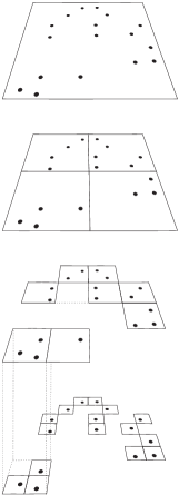
We employ the Barnes & Hut (1986, henceforth BH) tree construction in this work. In this scheme, the computational domain is hierarchically partitioned into a sequence of cubes, where each cube contains eight siblings, each with half the side-length of the parent cube. These cubes form the nodes of an oct-tree structure. The tree is constructed such that each node (cube) contains either exactly one particle, or is progenitor to further nodes, in which case the node carries the monopole and quadrupole moments of all the particles that lie inside its cube. A schematic illustration of the BH tree is shown in Figure 1.

A force computation then proceeds by walking the tree, and summing up appropriate force contributions from tree nodes. In the standard BH tree walk, the multipole expansion of a node of size $l$ is used only if

$$r>\frac{l}{\theta}\,,$$ (8)

where $r$ is the distance of the point of reference to the center-of-mass of the cell and $\theta$ is a prescribed accuracy parameter. If a node fulfills the criterion (8), the tree walk along this branch can be terminated, otherwise it is ‘opened’, and the walk is continued with all its siblings. For smaller values of the opening angle, the forces will in general become more accurate, but also more costly to compute. One can try to modify the opening criterion (8) to obtain higher efficiency, i.e. higher accuracy at a given length of the interaction list, something that we will discuss in more detail in Section 3.3.

A technical difficulty arises when the gravity is softened. In regions of high particle density (e.g. centers of dark haloes, or cold dense gas knots in dissipative simulations), it can happen that nodes fulfill equation (8), and simultaneously one has $r<h$, where $h$ is the gravitational softening length. In this situation, one formally needs the multipole moments of the softened gravitational field. One can work around this situation by opening nodes always for $r<h$, but this can slow down the code significantly if regions of very high particle density occur. Another solution is to use the proper multipole expansion for the softened potential, which we here discuss for definiteness. We want to approximate the potential at ${\bf r}$ due to a (distant) bunch of particles with masses $m_{i}$ and coordinates ${\bf x}_{i}$. We use a spline-softened force law, hence the exact potential of the particle group is

$$\Phi({\bf r})=-G\sum_{k}m_{k}\,g\left(\left|{\bf x}_{k}-{\bf r}\right|\right),$$ (9)

where the function $g(r)$ describes the softened force law. For Newtonian gravity we have $g(r)=1/r$, while the spline softened gravity with softening length $h$ gives rise to

$$g(r)=-\frac{1}{h}W_{2}\left(\frac{r}{h}\right).$$ (10)

The function $W_{2}(u)$ is given in the Appendix. It arises by replacing the force due to a point mass $m$ with the force exerted by the mass distribution $\rho({\bf r})=mW({\bf r};h)$, where we take $W(r;h)$ to be the normalized spline kernel used in the SPH formalism. The spline softening has the advantage that the force becomes exactly Newtonian for $r>h$, while some other possible force laws, like the Plummer softening, converge relatively slowly to Newton’s law.

Let ${\bf s}$ be the center-of-mass, and $M$ the total mass of the particles. Further we define ${\bf y}\equiv{\bf r}-{\bf s}$. The potential may then be expanded in a multipole series assuming $|{\bf y}|\gg|{\bf x}_{k}-{\bf s}|$. Up to quadrupole order, this results in

$$\Phi({\bf r}) = -G\bigg{\{}Mg(y)$$

$$\left.\;\;\;\;\;\;\;\;\;+\frac{1}{2}{\bf y}^{T}\left[\frac{g^{\prime\prime}(y)}{y^{2}}{\bf Q}+\frac{g^{\prime}(y)}{y^{3}}({\bf P}-{\bf Q})\right]{\bf y}\right\}.$$

Here we have introduced the tensors

$${\bf Q}=\sum_{k}m_{k}({\bf x}_{k}-{\bf s})({\bf x}_{k}-{\bf s})^{T}=\sum_{k}m_{k}{\bf x}_{k}\,{\bf x}_{k}^{T}-M{\bf s}\,{\bf s}^{T},$$ (12)

and

$${\bf P}={\bf I}\sum_{k}m_{k}({\bf x}_{k}-{\bf s})^{2}={\bf I}\left[\sum_{k}m_{k}{\bf x}_{k}^{2}-M{\bf s}^{2}\right],$$ (13)

where ${\bf I}$ is the unit matrix. Note that for Newtonian gravity, equation (3.1) reduces to the more familiar form

$$\Phi({\bf r})=-G\left[\frac{M}{y}+\frac{1}{2}{\bf y}^{T}\frac{\,\,3{\bf Q}-{\bf P}\,\,}{y^{5}}{\bf y}\right].$$ (14)

Finally, the quadrupole approximation of the softened gravitational field is given by

$${\bf f}({\bf r})=-\nabla\Phi=G\Big{\{}Mg_{1}(y){\bf y}+g_{2}(y){\bf Q}{\bf y}$$

$$\hskip 39.83368pt\left.+\frac{1}{2}g_{3}(y)\left({\bf y}^{T}{\bf Q}{\bf y}\right){\bf y}+\frac{1}{2}g_{4}(y){\bf P}{\bf y}\right\}.$$ (15)

Here we introduced the functions $g_{1}(y)$, $g_{2}(y)$, $g_{3}(y)$, and $g_{4}(y)$ as convenient abbreviations. Their definition is given in the Appendix. In the Newtonian case, this simplifies to

$${\bf f}({\bf r})=G\left\{-\frac{M}{y^{3}}{\bf y}+\frac{3{\bf Q}}{y^{5}}{\bf y}-\frac{15}{2}\frac{{\bf y}^{T}{\bf Q}{\bf y}}{y^{7}}{\bf y}+\frac{3}{2}\frac{{\bf P}}{y^{5}}{\bf y}\right\}.$$ (16)

Note that although equation (3.1) looks rather cumbersome, its actual numerical computation is only marginally more costly than that of the Newtonian form (16) because all factors involving $g(y)$ and derivatives thereof can be tabulated for later use in repeated force calculations.

3.2 Tree construction and tree walks

The tree construction can be done by inserting the particles one after the other in the tree. Once the grouping is completed, the multipole moments of each node can be recursively computed from the moments of its daughter nodes (McMillan & Aarseth 1993).

In order to reduce the storage requirements for tree nodes, we use single-precision floating point numbers to store node properties. The precision of the resulting forces is still fully sufficient for collisionless dynamics as long as the node properties are calculated accurately enough. In the recursive calculation, node properties will be computed from nodes that are already stored in single precision. When the particle number becomes very large (note that more than 10 million particles can be used in single objects like clusters these days), loss of sufficient precision can then result for certain particle distributions. In order to avoid this problem, GADGET optionally uses an alternative method to compute the node properties. In this method, a link-list structure is used to access all of the particles represented by each tree node, allowing a computation of the node properties in double-precision and a storage of the results in single-precision. While this technique guarantees that node properties are accurate up to a relative error of about $10^{-6}$, it is also slower than the recursive computation, because it requires of order $\cal{O}(N\log N)$ operations, while the recursive method is only of order $\cal{O}(N)$.

The tree-construction can be considered very fast in both cases, because the time spent for it is negligible compared to a complete force walk for all particles. However, in the individual time integration scheme only a small fraction of all particles may require a force walk at each given timestep. If this fraction drops below $\sim 1$ per cent, a full reconstruction of the tree can take as much time as the force walk itself. Fortunately, most of this tree construction time can be eliminated by dynamic tree updates (McMillan & Aarseth 1993), which we discuss in more detail in Section 5. The most time consuming routine in the code will then always remain the tree walk, and optimizing it can considerably speed up tree codes. Interestingly, in the grouping technique of Barnes (1990), the speed of the gravitational force computation can be increased by performing a common tree-walk for a localized group of particles. Even though the average length of the interaction list for each particles becomes larger in this way, this can be offset by saving some of the tree-walk overhead, and by improved cache utilization. Unfortunately, this advantage is not easily kept if individual timesteps are used, where only a small fraction of the particles are active, so we do not use grouping.

GADGET allows different gravitational softenings for particles of different ‘type’. In order to guarantee momentum conservation, this requires a symmetrization of the force when particles with different softening lengths interact. We symmetrize the softenings in the form

$$h=\max(h_{i},h_{j}).$$ (17)

However, the usage of different softening lengths leads to complications for softened tree nodes, because strictly speaking, the multipole expansion is only valid if all the particles in the node have the same softening. GADGET solves this problem by constructing separate trees for each species of particles with different softening. As long as these species are more or less spatially separated (e.g. dark halo, stellar disk, and stellar bulge in simulations of interacting galaxies), no severe performance penalty results. However, this is different if the fluids are spatially well ‘mixed’. Here a single tree would result in higher performance of the gravity computation, so it is advisable to choose a single softening in this case. Note that for SPH particles we nevertheless always create a separate tree to allow its use for a fast neighbour search, as will be discussed below.

3.3 Cell-opening criterion

The accuracy of the force resulting from a tree walk depends sensitively on the criterion used to decide whether the multipole approximation for a given node is acceptable, or whether the node has to be ‘opened’ for further refinement. The standard BH opening criterion tries to limit the relative error of every particle-node interaction by comparing a rough estimate of the size of the quadrupole term, $\sim Ml^{2}/r^{4}$, with the size of the monopole term, $\sim M/r^{2}$. The result is the purely geometrical criterion of equation (8).

However, as Salmon & Warren (1994) have pointed out, the worst-case behaviour of the BH criterion for commonly employed opening angles is somewhat worrying. Although typically very rare in real astrophysical simulations, the geometrical criterion (8) can then sometimes lead to very large force errors. In order to cure this problem, a number of modifications of the cell-opening criterion have been proposed. For example, Dubinski et al. (1996) have used the simple modification $r>{l}/{\theta}+\delta$, where the quantity $\delta$ gives the distance of the geometric center of the cell to its center-of-mass. This provides protection against pathological cases where the center-of-mass lies close to an edge of a cell.

Such modifications can help to reduce the rate at which large force errors occur, but they usually do not help to deal with another problem that arises for geometric opening criteria in the context of cosmological simulations at high redshift. Here, the density field is very close to being homogeneous and the peculiar accelerations are small. For a tree algorithm this is a surprisingly tough problem, because the tree code always has to sum up partial forces from all the mass in a simulation. Small net forces at high $z$ then arise in a delicate cancellation process between relatively large partial forces. If a partial force is indeed much larger than the net force, even a small relative error in it is enough to result in a large relative error of the net force. For an unclustered particle distribution, the BH criterion therefore requires a much smaller value of the opening angle than for a clustered one in order to achieve a similar level of force accuracy. Also note that in a cosmological simulation the absolute sizes of forces between a given particle and tree-nodes of a certain opening angle can vary by many orders of magnitude. In this situation, the purely geometrical BH criterion may end up investing a lot of computational effort for the evaluation of all partial forces to the same relative accuracy, irrespective of the actual size of each partial force and the size of the absolute error thus induced. It would be better to invest more computational effort in regions that provide most of the force on the particle and less in regions whose mass content is unimportant for the total force.

As suggested by Salmon & Warren (1994), one may therefore try to devise a cell-opening criterion that limits the absolute error in every cell-particle interaction. In principle, one can use analytic error bounds (Salmon & Warren 1994) to obtain a suitable cell-opening criterion, but the evaluation of the relevant expressions can consume significant amounts of CPU time.

Our approach to a new opening criterion is less stringent. Assume the absolute size of the true total force is already known before the tree walk. In the present code, we will use the acceleration of the previous timestep as a handy approximate value for that. We will now require that the estimated error of an acceptable multipole approximation is some small fraction of this total force. Since we truncate the multipole expansion at quadrupole order, the octupole moment will in general be the largest term in the neglected part of the series, except when the mass distribution in the cubical cell is close to being homogeneous. For a homogeneous cube the octupole moment vanishes by symmetry (Barnes & Hut 1989), such that the hexadecapole moment forms the leading term. We may very roughly estimate the size of these terms as $\sim M/r^{2}(l/r)^{3}$, or $\sim M/r^{2}(l/r)^{4}$, respectively, and take this as a rough estimate of the size of the truncation error. We can then require that this error should not exceed some fraction $\alpha$ of the total force on the particle, where the latter is estimated from the previous timestep. Assuming the octupole scaling, a tree-node has then to be opened if $M\,l^{3}>\alpha|{\bf a}_{\rm old}|r^{5}$. However, we have found that in practice the opening criterion

$$M\,l^{4}>\alpha|{\bf a}_{\rm old}|r^{6}\,$$ (18)

provides still better performance in the sense that it produces forces that are more accurate at a given computational expense. It is also somewhat cheaper to evaluate during the tree-walk, because $r^{6}$ is simpler to compute than $r^{5}$, which requires the evaluation of a root of the squared node distance. The criterion (18) does not suffer from the high-$z$ problem discussed above, because the same value of $\alpha$ produces a comparable force accuracy, independent of the clustering state of the material. However, we still need to compute the very first force using the BH criterion. In Section 7.2, we will show some quantitative measurements of the relative performance of the two criteria, and compare it to the optimum cell-opening strategy.

Note that the criterion (18) is not completely safe from worst-case force errors either. In particular, such errors can occur for opening angles so large that the point of force evaluation falls into the node itself. If this happens, no upper bound on the force error can be guaranteed (Salmon & Warren 1994). As an option to the code, we therefore combine the opening criterion (18) with the requirement that the point of reference may not lie inside the node itself. We formulate this additional constraint in terms of $r>b_{\rm max}$, where $b_{\rm max}$ is the maximum distance of the center-of-mass from any point in the cell. This additional geometrical constraint provides a very conservative control of force errors if this is needed, but increases the number of opened cells.

3.4 Special purpose hardware

An alternative to software solutions to the $N^{2}$-bottleneck of self-gravity is provided by the GRAPE (GRAvity PipE) special-purpose hardware. It is designed to solve the gravitational N-body problem in a direct summation approach by means of its superior computational speed. The latter is achieved with custom chips that compute the gravitational force with a hardwired Plummer force law. The Plummer-potential of GRAPE takes the form

$$\Phi({\bf r})=-G\sum_{j}\frac{m_{j}}{\left(|{\bf r}-{\bf r}_{j}|^{2}+\epsilon^{2}\right)^{\frac{1}{2}}}.$$ (19)

As an example, the GRAPE-3A boards installed at the MPA in 1998 have 40 N-body integrator chips in total with an approximate peak performance of 25 GFlops. Recently, newer generations of GRAPE boards have achieved even higher computational speeds. In fact, with the GRAPE-4 the 1 TFlop barrier was broken (Makino et al. 1997), and even faster special-purpose machines are in preparation (Hut & Makino 1999; Makino 2000). The most recent generation, GRAPE-6, can not only compute accelerations, but also its first and second time derivatives. Together with the capability to perform particle predictions, these machines are ideal for high-order Hermite integration schemes applied in simulations of collisional systems like star clusters. However, our present code is only adapted to the somewhat older GRAPE-3 (Okumura et al. 1993), and the following discussion is limited to it.

The GRAPE-3A boards are connected to an ordinary workstation via a VME or PCI interface. The boards consist of memory chips that can hold up to 131072 particle coordinates, and of integrator chips that can compute the forces exerted by these particles for 40 positions in parallel. Higher particle numbers can be processed by splitting them up in sufficiently small groups. In addition to the gravitational force, the GRAPE board returns the potential, and a list of neighbours for the 40 positions within search radii $h_{i}$ specified by the user. This latter feature makes GRAPE attractive also for SPH calculations.

The parts of our code that use GRAPE have benefited from the code GRAPESPH by Steinmetz (1996), and are similar to it. In short, the usage of GRAPE proceeds as follows. For the force computation, the particle coordinates are first loaded onto the GRAPE board, then GADGET calls GRAPE repeatedly to compute the force for up to 40 positions in parallel. The communication with GRAPE is done by means of a convenient software interface in C. GRAPE can also provide lists of nearest neighbours. For SPH-particles, GADGET computes the gravitational force and the interaction list in just one call of GRAPE. The host computer then still does the rest of the work, i.e. it advances the particles, and computes the hydrodynamical forces.

In practice, there are some technical complications when one works with GRAPE-3. In order to achieve high computational speed, the GRAPE-3 hardware works internally with special fixed-point formats for positions, accelerations and masses. This results in a reduced dynamic range compared to standard IEEE floating point arithmetic. In particular, one needs to specify a minimum length scale $d_{\rm min}$ and a minimum mass scale $m_{\rm min}$ when working with GRAPE. The spatial dynamic range is then given by $d_{\rm min}[-2^{18};2^{18}]$ and the mass range is $m_{\rm min}[1;64{\epsilon}/{d_{\rm min}}]$ (Steinmetz 1996).

While the communication time with GRAPE scales proportional to the particle number $N$, the actual force computation of GRAPE is still an ${\cal O}(N^{2})$-algorithm, because the GRAPE board implements a direct summation approach to the gravitational N-body problem. This implies that for very large particle number a tree code running on the workstation alone will eventually catch up and outperform the combination of workstation and GRAPE. For our current set-up at MPA this break-even point is about at 300000 particles.

However, it is also possible to combine GRAPE with a tree algorithm (Fukushige et al. 1991; Makino 1991a; Athanassoula et al. 1998; Kawai et al. 2000), for example by exporting tree nodes instead of particles in an appropriate way. Such a combination of tree+GRAPE scales as ${\cal O}(N\log N)$ and is able to outperform pure software solutions even for large $N$.

4 Smoothed particle hydrodynamics

SPH is a powerful Lagrangian technique to solve hydrodynamical problems with an ease that is unmatched by grid based fluid solvers (see Monaghan 1992, for an excellent review). In particular, SPH is very well suited for three-dimensional astrophysical problems that do not crucially rely on accurately resolved shock fronts.

Unlike other numerical approaches for hydrodynamics, the SPH equations do not take a unique form. Instead, many formally different versions of them can be derived. Furthermore, a large variety of recipes for specific implementations of force symmetrization, determinations of smoothing lengths, and artificial viscosity, have been described. Some of these choices are crucial for the accuracy and efficiency of the SPH implementation, others are only of minor importance. See the recent work by Thacker et al. (2000) and Lombardi et al. (1999) for a discussion of the relative performance of some of these possibilities. Below we give a summary of the specific SPH implementation we use.

4.1 Basic equations

The computation of the hydrodynamic force and the rate of change of internal energy proceeds in two phases. In the first phase, new smoothing lengths $h_{i}$ are determined for the active particles (these are the ones that need a force update at the current timestep, see below), and for each of them, the neighbouring particles inside their respective smoothing radii are found. The Lagrangian nature of SPH arises when this number of neighbours is kept either exactly, or at least roughly, constant. This is achieved by varying the smoothing length $h_{i}$ of each particle accordingly. The $h_{i}$ thus adjust to the local particle density adaptively, leading to a constant mass resolution independent of the density of the flow. Nelson & Papaloizou (1994) argue that it is actually best to keep the number of neighbours exactly constant, resulting in the lowest level of noise in SPH estimates of fluid quantities, and in the best conservation of energy. In practice, similarly good results are obtained if the fluctuations in neighbour number remain very small. In the serial version of GADGET we keep the number of neighbours fixed, whereas it is allowed to vary in a small band in the parallel code.

Having found the neighbours, we compute the density of the active particles as

$$\rho_{i}=\sum_{j=1}^{N}m_{j}W({\bf r}_{ij};h_{i}),$$ (20)

where ${\bf r}_{ij}\equiv{\bf r}_{i}-{\bf r}_{j}$, and we compute a new estimate of divergence and vorticity as

$$\rho_{i}(\nabla\cdot{\bf v})_{i}=\sum_{j}m_{j}({\bf v}_{j}-{\bf v}_{i})\nabla_{i}W({\bf r}_{ij};h_{i}),$$ (21)

$$\rho_{i}(\nabla\times{\bf v})_{i}=\sum_{j}m_{j}({\bf v}_{i}-{\bf v}_{j})\times\nabla_{i}W({\bf r}_{ij};h_{i}).$$ (22)

Here we employ the gather formulation for adaptive smoothing (Hernquist & Katz 1989).

For the passive particles, values for density, internal energy, and smoothing length are predicted at the current time based on the values of the last update of those particles (see Section 5). Finally, the pressure of the particles is set to $P_{i}=(\gamma-1)\rho_{i}u_{i}$.

In the second phase, the actual forces are computed. Here we symmetrize the kernels of gather and scatter formulations as in Hernquist & Katz (1989). We compute the gasdynamical accelerations as

$${\bf a}_{i}^{\rm gas}=-\left(\frac{\nabla P}{\rho}\right)_{i}+{\bf a}_{i}^{\rm visc}=-\sum_{j}m_{j}\left(\frac{P_{i}}{\rho_{i}^{2}}+\frac{P_{j}}{\rho_{j}^{2}}+\tilde{\Pi}_{ij}\right)\$$

$$\left[\frac{1}{2}\nabla_{i}W({\bf r}_{ij};h_{i})+\frac{1}{2}\nabla_{i}W({\bf r}_{ij};h_{j})\right],$$ (23)

and the change of the internal energy as

$$\frac{{\rm d}u_{i}}{{\rm d}t}=\frac{1}{2}\sum_{j}m_{j}\left(\frac{P_{i}}{\rho_{i}^{2}}+\frac{P_{j}}{\rho_{j}^{2}}+\tilde{\Pi}_{ij}\right)({\bf v}_{i}-{\bf v}_{j})\,$$

$$\left[\frac{1}{2}\nabla_{i}W({\bf r}_{ij};h_{i})+\frac{1}{2}\nabla_{i}W({\bf r}_{ij};h_{j})\right].$$ (24)

Instead of symmetrizing the pressure terms with an arithmetic mean, the code can also be used with a geometric mean according to

$$\frac{P_{i}}{\rho_{i}^{2}}+\frac{P_{j}}{\rho_{j}^{2}}\;\;\longrightarrow\;\;2\frac{\sqrt{P_{i}P_{j}}}{\rho_{i}\rho_{j}}.$$ (25)

This may be slightly more robust in certain situations (Hernquist & Katz 1989). The artificial viscosity $\tilde{\Pi}_{ij}$ is taken to be

$$\tilde{\Pi}_{ij}=\frac{1}{2}(f_{i}+f_{j})\Pi_{ij},$$ (26)

with

$$\Pi_{ij}=\left\{\begin{tabular}[]{cl}${\left[-\alpha c_{ij}\mu_{ij}+2\alpha\mu_{ij}^{2}\right]}/{\rho_{ij}}$&\mbox{if ${\bf v}_{ij}\cdot{\bf r}_{ij}<0$}\\ 0&\mbox{otherwise},\\ \end{tabular}\right.$$ (27)

where

$$f_{i}=\frac{|(\nabla\cdot{\bf v})_{i}|}{|(\nabla\cdot{\bf v})_{i}|+|(\nabla\times{\bf v})_{i}|},$$ (28)

and

$$\mu_{ij}=\frac{h_{ij}({\bf v}_{i}-{\bf v}_{j})({\bf r}_{i}-{\bf r}_{j})}{\left|{\bf r}_{i}-{\bf r}_{j}\right|^{2}+\epsilon h_{ij}^{2}}.$$ (29)

This form of artificial viscosity is the shear-reduced version (Balsara 1995; Steinmetz 1996) of the ‘standard’ Monaghan & Gingold (1983) artificial viscosity. Recent studies (Lombardi et al. 1999; Thacker et al. 2000) that test SPH implementations endorse it.

In equations (4.1) and (4.1), a given SPH particle $i$ will interact with a particle $j$ whenever $|{\bf r}_{ij}|<h_{i}$ or $|{\bf r}_{ij}|<h_{j}$. Standard search techniques can relatively easily find all neighbours of particle $i$ inside a sphere of radius $h_{i}$, but making sure that one really finds all interacting pairs in the case $h_{j}>h_{i}$ is slightly more tricky. One solution to this problem is to simply find all neighbours of $i$ inside $h_{i}$, and to consider the force components

$${\bf f}_{ij}=-m_{i}m_{j}\left(\frac{P_{i}}{\rho_{i}^{2}}+\frac{P_{j}}{\rho_{j}^{2}}+\tilde{\Pi}_{ij}\right)\frac{1}{2}\nabla_{i}W({\bf r}_{ij};h_{i}).$$ (30)

If we add ${\bf f}_{ij}$ to the force on $i$, and $-{\bf f}_{ij}$ to the force on $j$, the sum of equation (4.1) is reproduced, and the momentum conservation is manifest. This also holds for the internal energy. Unfortunately, this only works if all particles are active. In an individual timestep scheme, we therefore need an efficient way to find all the neighbours of particle $i$ in the above sense, and we discuss our algorithm for doing this below.

4.2 Neighbour search

In SPH, a basic task is to find the nearest neighbours of each SPH particle to construct its interaction list. Specifically, in the implementation we have chosen we need to find all particles closer than a search radius $h_{i}$ in order to estimate the density, and one needs all particles with $|{\bf r}_{ij}|<\max(h_{i},h_{j})$ for the estimation of hydrodynamical forces. Similar to gravity, the naive solution that checks the distance of all particle pairs is an ${\cal O}(N^{2})$ algorithm which slows down prohibitively for large particle numbers. Fortunately, there are faster search algorithms.

When the particle distribution is approximately homogeneous, perhaps the fastest algorithms work with a search grid that has a cell size somewhat smaller than the search radius. The particles are then first coarse-binned onto this search grid, and link-lists are established that quickly deliver only those particles that lie in a specific cell of the coarse grid. The neighbour search proceeds then by range searching; only those mesh cells that have a spatial overlap with the search range have to be opened.

For highly clustered particle distributions and varying search ranges $h_{i}$, the above approach quickly degrades, since the mesh chosen for the coarse grid has not the optimum size for all particles. A more flexible alternative is to employ a geometric search tree. For this purpose, a tree with a structure just like the BH oct-tree can be employed, Hernquist & Katz (1989) were the first to use the gravity tree for this purpose. In GADGET we use the same strategy and perform a neighbour search by walking the tree. A cell is ‘opened’ (i.e. further followed) if it has a spatial overlap with the rectangular search range. Testing for such an overlap is faster with a rectangular search range than with a spherical one, so we inscribe the spherical search region into a little cube for the purpose of this walk. If one arrives at a cell with only one particle, this is added to the interaction list if it lies inside the search radius. We also terminate a tree walk along a branch, if the cell lies completely inside the search range. Then all the particles in the cell can be added to the interaction list, without checking any of them for overlap with the search range any more. The particles in the cell can be retrieved quickly by means of a link-list, which can be constructed along with the tree and allows a retrieval of all the particles that lie inside a given cell, just as it is possible in the coarse-binning approach. Since this short-cut reduces the length of the tree walk and the number of required checks for range overlap, the speed of the algorithm is increased by a significant amount.

With a slight modification of the tree walk, one can also find all particles with $|{\bf r}_{ij}|<\max(h_{i},h_{j})$. For this purpose, we store in each tree node the maximum SPH smoothing length occurring among its particles. The test for overlap is then simply done between a cube of side-length $\max(h_{i},h_{\rm node})$ centered on the particle $i$ and the node itself, where $h_{\rm node}$ is the maximum smoothing length among the particles of the node.

There remains the task to keep the number of neighbours around a given SPH particle approximately (or exactly) constant. We solve this by predicting a value $\tilde{h}_{i}$ for the smoothing length based on the length $h_{i}$ of the previous timestep, the actual number of neighbours $N_{i}$ at that timestep, and the local velocity divergence:

$$\tilde{h}_{i}=\frac{1}{2}h_{i}^{\rm(old)}\left[1+\left(\frac{N_{\rm s}}{N_{i}}\right)^{1/3}\right]+\dot{h}_{i}\,\Delta t,$$ (31)

where $\dot{h}_{i}=\frac{1}{3}h_{i}(\nabla\cdot{\bf v})_{i}$, and $N_{\rm s}$ is the desired number of neighbours. A similar form for updating the smoothing lengths has been used by Hernquist & Katz (1989), see also Thacker et al. (2000) for a discussion of alternative choices. The term in brackets tries to bring the number of neighbours back to the desired value if $N_{i}$ deviates from it. Should the resulting number of neighbours nevertheless fall outside a prescribed range of tolerance, we iteratively adjust ${h}_{i}$ until the number of neighbours is again brought back to the desired range. Optionally, our code allows the user to impose a minimum smoothing length for SPH, typically chosen as some fraction of the gravitational softening length. A larger number of neighbours than $N_{\rm s}$ is allowed to occur if $h_{i}$ takes on this minimum value.

One may also decide to keep the number of neighbours exactly constant by defining $h_{i}$ to be the distance to the $N_{\rm s}$-nearest particle. We employ such a scheme in the serial code. Here we carry out a range-search with $R=1.2\tilde{h}_{i}$, on average resulting in $\sim 2N_{\rm s}$ potential neighbours. From these we select the closest $N_{\rm s}$ (fast algorithms for doing this exist, see Press et al. 1995). If there are fewer than $N_{\rm s}$ particles in the search range, or if the distance of the $N_{\rm s}$-nearest particle inside the search range is larger than $R$, the search is repeated for a larger search range. In the first timestep no previous $h_{i}$ is known, so we follow the neighbour tree backwards from the leaf of the particle under consideration, until we obtain a first reasonable guess for the local particle density (based on the number $N$ of particles in a node of volume $l^{3}$), providing an initial guess for $\tilde{h}_{i}$.

However, the above scheme for keeping the number of neighbours exactly fixed is not easily accommodated in our parallel SPH implementation, because SPH particles may have a search radius that overlaps with several processor domains. In this case, the selection of the closest $N_{\rm s}$ neighbours becomes non-trivial, because the underlying data is distributed across several independent processor elements. For parallel SPH, we therefore revert to the simpler scheme and allow the number of neighbours to fluctuate within a small band.

5 Time integration

As a time integrator, we use a variant of the leapfrog involving an explicit prediction step. The latter is introduced to accommodate individual particle timesteps in the N-body scheme, as explained later on.

We start by describing the integrator for a single particle. First, a particle position at the middle of the timestep $\Delta t$ is predicted according to

$$\tilde{\bf r}^{(n+\frac{1}{2})}={\bf r}^{(n)}+{\bf v}^{(n)}\frac{\Delta t}{2},$$ (32)

and an acceleration based on this position is computed, viz.

$${\bf a}^{({n}+\frac{1}{2})}=-\left.\nabla\Phi\right|_{\tilde{\bf r}^{({n}+\frac{1}{2})}}.$$ (33)

Then the particle is advanced according to

$${\bf v}^{(n+1)}={\bf v}^{(n)}+{\bf a}^{({n}+\frac{1}{2})}\Delta t,$$ (34)

$${\bf r}^{({n}+1)}={\bf r}^{({n})}+\frac{1}{2}\left[{\bf v}^{({n})}+{\bf v}^{({n}+1)}\right]\Delta t.$$ (35)

5.1 Timestep criterion

In the above scheme, the timestep may vary from step to step. It is clear that the choice of timestep size is very important in determining the overall accuracy and computational efficiency of the integration.

In a static potential $\Phi$, the error in specific energy arising in one step with the above integrator is

$$\Delta E = \frac{1}{4}\frac{\partial^{2}\Phi}{\partial x_{i}\partial x_{j}}v_{i}^{(n)}a^{(n+\frac{1}{2})}_{j}\Delta t^{3}+$$

$$\frac{1}{24}\frac{\partial^{3}\Phi}{\partial x_{i}\partial x_{j}\partial x_{k}}v^{(n)}_{i}v^{(n)}_{j}v^{(n)}_{k}\Delta t^{3}+{\cal O}(\Delta t^{4})$$

to leading order in $\Delta t$, i.e. the integrator is second order accurate. Here the derivatives of the potential are taken at coordinate ${\bf r}^{(n)}$ and summation over repeated coordinate indices is understood.

In principle, one could try to use equation (5.1) directly to obtain a timestep by imposing some upper limit on the tolerable error $\Delta E$. However, this approach is quite subtle in practice. First, the derivatives of the potential are difficult to obtain, and second, there is no explicit guarantee that the terms of higher order in $\Delta t$ are really small.

High-order Hermite schemes use timestep criteria that include the first and second time derivative of the acceleration (e.g. Makino 1991b; Makino & Aarseth 1992). While these timestep criteria are highly successful for the integration of very nonlinear systems, they are probably not appropriate for our low-order scheme, apart from the fact that substantial computational effort is required to evaluate these quantities directly. Ideally, we therefore want to use a timestep criterion that is only based on dynamical quantities that are either already at hand or are relatively cheap to compute.

Note that a well known problem of adaptive timestep schemes is that they will usually break the time reversibility and symplectic nature of the simple leapfrog. As a result, the system does not evolve under a pseudo-Hamiltonian any more and secular drifts in the total energy can occur. As Quinn et al. (1997) show, reversibility can be obtained with a timestep that depends only on the relative coordinates of particles. This is for example the case for timesteps that depend only on acceleration or on local density. However, to achieve reversibility the timestep needs to be chosen based on the state of the system in the middle of the timestep (Quinn et al. 1997), or on the beginning and end of the timestep (Hut et al. 1995). In practice, this can be accomplished by discarding trial timesteps appropriately. The present code selects the timestep based on the previous step and is thus not reversible in this way.

One possible timestep criterion is obtained by constraining the absolute size of the second order displacement of the kinetic energy, assuming a typical velocity dispersion $\sigma^{2}$ for the particles, which corresponds to a scale $E=\sigma^{2}$ for the typical specific energy. This results in

$$\Delta t=\alpha_{\rm tol}\frac{\sigma}{|{\bf a}|}.$$ (37)

For a collisionless fluid, the velocity scale $\sigma$ should ideally be chosen as the local velocity dispersion, leading to smaller timesteps in smaller haloes, or more generally, in ‘colder’ parts of the fluid. The local velocity dispersion can be estimated from a local neighbourhood of particles, obtained as in the normal SPH formalism.

Alternatively, one can constrain the second order term in the particle displacement, obtaining

$$\Delta t=\sqrt{\frac{2\alpha^{\prime}_{\rm tol}\epsilon}{|{\bf a}|}}.$$ (38)

Here some length scale $\alpha^{\prime}_{\rm tol}\epsilon$ is introduced, which will typically be related to the gravitational softening. This form has quite often been employed in cosmological simulations, sometimes with an additional restriction on the displacement of particles in the form $\Delta t=\tilde{\alpha}\epsilon/|{\bf v}|$. It is unclear though why the timesteps should depend on the gravitational softening length in this way. In a well-resolved halo, most orbits are not expected to change much if the halo is modeled with more particles and a correspondingly smaller softening length, so it should not be necessary to increase the accuracy of the time integration for all particles by the same factor if the mass/length resolution is increased.

For self-gravitating collisionless fluids, another plausible timestep criterion is based on the local dynamical time:

$$\Delta t=\alpha^{\prime\prime}_{\rm tol}\frac{3}{\sqrt{8\pi G\rho}}.$$ (39)

One advantage of this criterion is that it provides a monotonically decreasing timestep towards the center of a halo. On the other hand, it requires an accurate estimate of the local density, which may be difficult to obtain, especially in regions of low density. In particular, Quinn et al. (1997) have shown that haloes in cosmological simulations that contain only a small number of particles, about equal or less than the number employed to estimate the local density, are susceptible to destruction if a timestep based on (39) is used. This is because the kernel estimates of the density are too small in this situation, leading to excessively long timesteps in these haloes.

In simple test integrations of singular potentials, we have found the criterion (37) to give better results compared to the alternative (38). However, neither of these simple criteria is free of problems in typical applications to structure formation, as we will later show in some test calculations. In the center of haloes, subtle secular effects can occur under conditions of coarse integration settings. The criterion based on the dynamical time does better in this respect, but it does not work well in regions of very low density. We thus suggest to use a combination of (37) and (39) by taking the minimum of the two timesteps. This provides good integration accuracy in low density environments and simultaneously does well in the central regions of large haloes. For the relative setting of the dimensionless tolerance parameters we use $\alpha^{\prime\prime}\simeq 3\alpha$, which typically results in a situation where roughly the same number of particles are constrained by each of the two criteria in an evolved cosmological simulation. The combined criterion is Galilean-invariant and does not make an explicit reference to the gravitational softening length employed.

5.2 Integrator for N-body systems

In the context of stellar dynamical integrations, individual particle timesteps have long been used since they were first introduced by Aarseth (1963). We here employ an integrator with completely flexible timesteps, similar to the one used by Groom (1997) and Hiotelis & Voglis (1991). This scheme differs slightly from more commonly employed binary hierarchies of timesteps (e.g. Hernquist & Katz 1989; McMillan & Aarseth 1993; Steinmetz 1996).

Each particle has a timestep $\Delta t_{i}$, and a current time $t_{i}$, where its dynamical state (${\bf r}_{i}$, ${\bf v}_{i}$, ${\bf a}_{i}$) is stored. The dynamical state of the particle can be predicted at times $t\in[t_{i}\pm 0.5\Delta t_{i}]$ with first order accuracy.

The next particle $k$ to be advanced is then the one with the minimum prediction time defined as $\tau_{\rm p}\equiv{\rm min}\left(t_{i}+0.5\Delta t_{i}\right)$. The time $\tau_{\rm p}$ becomes the new current time of the system. To advance the corresponding particle, we first predict positions for all particles at time $\tau_{\rm p}$ according to

$$\tilde{\bf r}_{i}={\bf r}_{i}+{\bf v}_{i}(\tau_{\rm p}-t_{i}).$$ (40)

Based on these positions, the acceleration of particle $k$ at the middle of its timestep is calculated as

$${\bf a}_{k}^{({n}+\frac{1}{2})}=-\left.\nabla\Phi(\tilde{\bf r}_{i})\right|_{\tilde{\bf r}_{k}}.$$ (41)

Position and velocity of particle $k$ are then advanced as

$${\bf v}^{(n+1)}_{k}={\bf v}^{(n)}_{k}+2{\bf a}_{k}^{({n}+\frac{1}{2})}(\tau_{\rm p}-t_{k}),$$ (42)

$${\bf r}^{(n+1)}_{k}={\bf r}^{(n)}_{k}+\left[{\bf v}^{(n)}_{k}+{\bf v}^{({n}+1)}_{k}\right](\tau_{\rm p}-t_{k}),$$ (43)

and its current time can be updated to

$$t_{k}^{(\rm new)}=t_{k}+2(\tau_{\rm p}-t_{k}).$$ (44)

Finally, a new timestep $\Delta t_{k}^{(\rm new)}$ for the particle is estimated.

At the beginning of the simulation, all particles start out with the same current time. However, since the timesteps of the particles are all different, the current times of the particles distribute themselves nearly symmetrically around the current prediction time, hence the prediction step involves forward and backward prediction to a similar extent.

Of course, it is impractical to advance only a single particle at any given prediction time, because the prediction itself and the (dynamic) tree updates induce some overhead. For this reason we advance particles in bunches. The particles may be thought of as being ordered according to their prediction times $t_{i}^{\rm p}=t_{i}+\frac{1}{2}\Delta t_{i}$. The simulation works through this time line, and always advances the particle with the smallest $t_{i}^{\rm p}$, and also all subsequent particles in the time line, until the first is found with

$$\tau_{\rm p}\leq t_{i}+\frac{1}{4}\Delta t_{i}\,.$$ (45)

This condition selects a group of particles at the lower end of the time line, and all the particles of the group are guaranteed to be advanced by at least half of their maximum allowed timestep. Compared to using a fixed block step scheme with a binary hierarchy, particles are on average advanced closer to their maximum allowed timestep in this scheme, which results in a slight improvement in efficiency. Also, timesteps can more gradually vary than in a power of two hierarchy. However, a perhaps more important advantage of this scheme is that it makes work-load balancing in the parallel code simpler, as we will discuss in more detail later on.

In practice, the size $M$ of the group that is advanced at a given step is often only a small fraction of the total particle number $N$. In this situation it becomes important to eliminate any overhead that scales with ${\cal O}(N)$. For example, we obviously need to find the particle with the minimum prediction time at every timestep, and also the particles following it in the time line. A loop over all the particles, or a complete sort at every timestep, would induce overhead of order ${\cal O}(N)$ or ${\cal O}(N\log N)$, which can become comparable to the force computation itself if $M/N\ll 1$. We solve this problem by keeping the maximum prediction times of the particles in an ordered binary tree (Wirth 1986) at all times. Finding the particle with the minimum prediction time and the ones that follow it are then operations of order ${\cal O}(\log N)$. Also, once the particles have been advanced, they can be removed and reinserted into this tree with a cost of order ${\cal O}(\log N)$. Together with the dynamic tree updates, which eliminate prediction and tree construction overhead, the cost of the timestep then scales as ${\cal O}(M\log N)$.

5.3 Dynamic tree updates

If the fraction of particles to be advanced at a given timestep is indeed small, the prediction of all particles and the reconstruction of the full tree would also lead to significant sources of overhead. However, as McMillan & Aarseth (1993) have first discussed, the geometric structure of the tree, i.e. the way the particles are grouped into a hierarchy, evolves only relatively slowly in time. It is therefore sufficient to reconstruct this grouping only every few timesteps, provided one can still obtain accurate node properties (center of mass, multipole moments) at the current prediction time.

We use such a scheme of dynamic tree updates by predicting properties of tree-nodes on the fly, instead of predicting all particles every single timestep. In order to do this, each node carries a center-of-mass velocity in addition to its position at the time of its construction. New node positions can then be predicted while the tree is walked, and only nodes that are actually visited need to be predicted. Note that the leaves of the tree point to single particles. If they are used in the force computation, their prediction corresponds to the ordinary prediction as outlined in equation (43).

In our simple scheme we neglect a possible time variation of the quadrupole moment of the nodes, which can be taken into account in principle (McMillan & Aarseth 1993). However, we introduce a mechanism that reacts to fast time variations of tree nodes. Whenever the center-of mass of a tree node under consideration has moved by more than a small fraction of the nodes’ side-length since the last reconstruction of this part of the tree, the node is completely updated, i.e. the center-of-mass, center-of-mass velocity and quadrupole moment are recomputed from the individual (predicted) phase-space variables of the particles. We also adjust the side-length of the tree node if any of its particles should have left its original cubical volume.

Finally, the full tree is reconstructed from scratch every once in a while to take into account the slow changes in the grouping hierarchy. Typically, we update the tree whenever a total of $\sim 0.1N$ force computations have been done since the last full reconstruction. With this criterion the tree construction is an unimportant fraction of the total computation time. We have not noticed any significant loss of force accuracy induced by this procedure.

In summary, the algorithms described above result in an integration scheme that can smoothly and efficiently evolve an N-body system containing a large dynamic range in time scales. At a given timestep, only a small number $M$ of particles are then advanced, and the total time required for that scales as ${\cal O}(M\log N)$.

5.4 Including SPH

The above time integration scheme may easily be extended to include SPH. Here we also need to integrate the internal energy equation, and the particle accelerations also receive a hydrodynamical component. To compute the latter we also need predicted velocities

$$\tilde{\bf v}_{i}={\bf v}_{i}+{\bf a}_{i-1}(\tau_{\rm p}-t_{i}),$$ (46)

where we have approximated ${\bf a}_{i}$ with the acceleration of the previous timestep. Similarly, we obtain predictions for the internal energy

$$\tilde{u}_{i}={u}_{i}+\dot{u}_{i}(\tau_{\rm p}-t_{i}),$$ (47)

and the density of inactive particles as

$$\tilde{\rho}_{i}={\rho}_{i}+\dot{\rho}_{i}(\tau_{\rm p}-t_{i}).$$ (48)

For those particles that are to be advanced at the current system step, these predicted quantities are then used to compute the hydrodynamical part of the acceleration and the rate of change of internal energy with the usual SPH estimates, as described in Section 4.

For hydrodynamical stability, the collisionless timestep criterion needs to be supplemented with the Courant condition. We adopt it for the gas particles in the form

$$\Delta t_{i}=\frac{\alpha_{\rm cour}\,h_{i}}{h_{i}|(\nabla\cdot{\bf v})_{i}|+\max(c_{i},|{\bf v}_{i}|)\,(1+0.6\,\alpha_{\rm visc})},$$ (49)

where $\alpha_{\rm visc}$ regulates the strength of the artificial bulk viscosity, and $\alpha_{\rm cour}$ is an accuracy parameter, the Courant factor. Note that we use the maximum of the sound speed $c_{i}$ and the bulk velocity $|{\bf v}_{i}|$ in this expression. This improves the handling of strong shocks when the infalling material is cold, but has the disadvantage of not being Galilean invariant. For the SPH-particles, we use either the adopted criterion for collisionless particles or (49), whichever gives the smaller timestep.

As defined above, we evaluate ${\bf a}^{\rm gas}$ and $\dot{u}$ at the middle of the timestep, when the actual timestep $\Delta t$ of the particle that will be advanced is already set. Note that there is a term in the artificial viscosity that can cause a problem in this explicit integration scheme. The second term in equation (27) tries to prevent particle inter-penetration. If a particle happens to get relatively close to another SPH particle in the time $\Delta t/2$ and the relative velocity of the approach is large, this term can suddenly lead to a very large repulsive acceleration ${\bf a}^{\rm visc}$, trying to prevent the particles from getting any closer. However, it is then too late to reduce the timestep. Instead, the velocity of the approaching particle will be changed by ${\bf a}^{\rm visc}\Delta t$, possibly reversing the approach of the two particles. But the artificial viscosity should at most halt the approach of the particles. To guarantee this, we introduce an upper cut-off to the maximum acceleration induced by the artificial viscosity. If ${\bf v}_{ij}\cdot{\bf r}_{ij}<0$, we replace equation (26) with

$$\tilde{\Pi}_{ij}=\frac{1}{2}(f_{i}+f_{j})\,\min\left[\Pi_{ij},\frac{{\bf v}_{ij}\cdot{\bf r}_{ij}}{(m_{i}+m_{j})W_{ij}\Delta t}\right],$$ (50)

where $W_{ij}={\bf r}_{ij}\nabla_{i}\left[W({\bf r}_{ij};h_{i})+W({\bf r}_{ij};h_{j})\right]/2$. With this change, the integration scheme still works reasonably well in regimes with strong shocks under conditions of relatively coarse timestepping. Of course, a small enough value of the Courant factor will prevent this situation from occurring to begin with.

Since we use the gravitational tree of the SPH particles for the neighbour search, another subtlety arises in the context of dynamic tree updates, where the full tree is not necessarily reconstructed every single timestep. The range searching technique relies on the current values of the maximum SPH smoothing length in each node, and also expects that all particles of a node are still inside the boundaries set by the side-length of a node. To guarantee that the neighbour search will always give correct results, we perform a special update of the SPH-tree every timestep. It involves a loop over every SPH particle that checks whether the particle’s smoothing length is larger than $h_{\rm max}$ stored in its parent node, or if it falls outside the extension of the parent node. If either of these is the case, the properties of the parent node are updated accordingly, and the tree is further followed ‘backwards’ along the parent nodes, until each node is again fully ‘contained’ in its parent node. While this update routine is very fast in general, it does add some overhead, proportional to the number of SPH particles, and thus breaks in principle the ideal scaling (proportional to $M$) obtained for purely collisionless simulations.

5.5 Implementation of cooling

When radiative cooling is included in simulations of galaxy formation or galaxy interaction, additional numerical problems arise. In regions of strong gas cooling, the cooling times can become so short that extremely small timesteps would be required to follow the internal energy accurately with the simple explicit integration scheme used so far.

To remedy this problem, we treat the cooling semi-implicitly in an isochoric approximation. At any given timestep, we first compute the rate $\dot{u}^{\rm ad}$ of change of the internal energy due to the ordinary adiabatic gas physics. In an isochoric approximation, we then solve implicitly for a new internal energy predicted at the end of the timestep, i.e.

$$\hat{u}_{i}^{(n+1)}=u_{i}^{(n)}+\dot{u}^{\rm ad}\Delta t-\frac{\Lambda\left[\rho_{i}^{(n)},\hat{u}_{i}^{(n+1)}\right]\Delta t}{\rho_{i}^{(n)}}\,.$$ (51)

The implicit computation of the cooling rate guarantees stability. Based on this estimate, we compute an effective rate of change of the internal energy, which we then take as

$$\dot{u}_{i}=\left[\hat{u}_{i}^{(n+1)}-u_{i}^{(n)}\right]/\Delta t\,.$$ (52)

We use this last step because the integration scheme requires the possibility to predict the internal energy at arbitrary times. With the above procedure, $u_{i}$ is always a continuous function of time, and the prediction of $u_{i}$ may be done for times in between the application of the isochoric cooling/heating. Still, there can be a problem with predicted internal energies in cases when the cooling time is very small. Then a particle can lose a large fraction of its energy in a single timestep. While the implicit solution will still give a correct result for the temperature at the end of the timestep, the predicted energy in the middle of the next timestep could then become very small or even negative because of the large negative value of $\dot{u}$. We therefore restrict the maximum cooling rate such that a particle is only allowed to lose at most half its internal energy in a given timestep, preventing the predicted energies from ‘overshooting’. Katz & Gunn (1991) have used a similar method to damp the cooling rate.

5.6 Integration in comoving coordinates

For simulations in a cosmological context, the expansion of the universe has to be taken into account. Let ${\bf x}$ denote comoving coordinates, and $a$ be the dimensionless scale factor ($a=1.0$ at the present epoch). Then the Newtonian equation of motion becomes

$$\ddot{{\bf x}}+2\frac{\dot{a}}{a}\,\dot{{\bf x}}=-G\int\frac{\delta\rho({\bf x}^{\prime})\,({\bf x}-{\bf x}^{\prime})}{|{\bf x}-{\bf x}^{\prime}|^{3}}{\rm d}^{3}x^{\prime}.$$ (53)

Here the function $\delta\rho({\bf x})=\rho({\bf x})-{\overline{\rho}}$ denotes the (proper) density fluctuation field.

In an N-body simulation with periodic boundary conditions, the volume integral of equation (53) is carried out over all space. As a consequence, the homogeneous contribution arising from ${\overline{\rho}}$ drops out around every point. Then the equation of motion of particle $i$ becomes

$$\ddot{{\bf x}}_{i}+2\frac{\dot{a}}{a}\,\dot{{\bf x}}_{i}=-\frac{G}{a^{3}}\sum_{j\neq i\atop{\rm periodic}}\frac{m_{j}\,({\bf x}_{i}-{\bf x}_{j})}{|{\bf x}_{i}-{\bf x}_{j}|^{3}},$$ (54)

where the summation includes all periodic images of the particles $j$.

However, one may also employ vacuum boundary conditions if one simulates a spherical region of radius $R$ around the origin, and neglects density fluctuations outside this region. In this case, the background density ${\overline{\rho}}$ gives rise to an additional term, viz.

$$\ddot{{\bf x}}_{i}+2\frac{\dot{a}}{a}\,\dot{{\bf x}}_{i}=\frac{1}{a^{3}}\left[-G\sum_{j\neq i}\frac{m_{j}\,{\bf x}_{ij}}{|{\bf x}_{ij}|^{3}}\,+\,\frac{1}{2}\Omega_{0}H_{0}^{2}{\bf x}_{i}\right].$$ (55)

GADGET supports both periodic and vacuum boundary conditions. We implement the former by means of the Ewald summation technique (Hernquist et al. 1991).

For this purpose, we modify the tree walk such that each node is mapped to the position of its nearest periodic image with respect to the coordinate under consideration. If the multipole expansion of the node can be used according to the cell opening criterion, its partial force is computed in the usual way. However, we also need to add the force exerted by all the other periodic images of the node. The slowly converging sum over these contributions can be evaluated with the Ewald technique. If ${\bf x}$ is the coordinate of the point of force-evaluation relative to a node of mass $M$, the resulting additional acceleration is given by

$${\bf a}_{c}({\bf x})=M\Bigg{\{}\frac{{\bf x}}{|{\bf x}|^{3}}-\sum_{\bf n}\frac{{\bf x}-{\bf n}L}{|{\bf x}-{\bf n}L|^{3}}\times\bigg{[}{\rm erfc}(\alpha|{\bf x}-{\bf n}L|)+$$

$$\frac{2\alpha|{\bf x}-{\bf n}L|}{\sqrt{\pi}}\exp\left(-\alpha^{2}|{\bf x}-{\bf n}L|^{2}\right)\bigg{]}$$

$$-\frac{2}{L^{2}}\sum_{{\bf h}\neq 0}\frac{{\bf h}}{|{\bf h}|^{2}}\exp\left(-\frac{\pi^{2}|{\bf h}|^{2}}{\alpha^{2}L^{2}}\right)\sin\left(\frac{2\pi}{L}{\bf h}\cdot{\bf x}\right)\Bigg{\}}.$$ (56)

Here ${\bf n}$ and ${\bf h}$ are integer triplets, $L$ is the box size, and $\alpha$ is an arbitrary number (Hernquist et al. 1991). Good convergence is achieved for $\alpha=2/L$, where we sum over the range $|{\bf n}|<5$ and $|{\bf h}|<5$. Similarly, the additional potential due to the periodic replications of the node is given by

$$\phi_{c}({\bf x})=M\bigg{\{}\frac{1}{{\bf x}}+\frac{\pi}{\alpha^{2}L^{3}}-\sum_{{\bf n}}\frac{{\rm erfc}(\alpha|{\bf x}-{\bf n}L|)}{|{\bf x}-{\bf n}L|}-$$

$$\frac{1}{L}\sum_{{\bf h}\neq 0}\frac{1}{\pi|{\bf h}|^{2}}\exp\left(-\frac{\pi^{2}|{\bf h}|^{2}}{\alpha^{2}L^{2}}\right)\cos\left(\frac{2\pi}{L}{\bf h}\cdot{\bf x}\right)\Bigg{\}}.$$ (57)

We follow Hernquist et al. (1991) and tabulate the correction fields ${\bf a}_{c}({\bf x})/M$ and $\phi_{c}({\bf x})/M$ for one octant of the simulation box, and obtain the result of the Ewald summation during the tree walk from trilinear interpolation off this grid. It should be noted however, that periodic boundaries have a strong impact on the speed of the tree algorithm. The number of floating point operations required to interpolate the correction forces from the grid has a significant toll on the raw force speed and can slow it down by almost a factor of two.

In linear theory, it can be shown that the kinetic energy

$$T=\frac{1}{2}\sum_{i}m_{i}{{\bf v}}^{2}$$ (58)

in peculiar motion grows proportional to $a$, at least at early times. This implies that $\sum_{i}m_{i}\dot{{\bf x}}^{2}\propto 1/a$, hence the comoving velocities $\dot{{\bf x}}={\bf v}/a$ actually diverge for $a\to 0$. Since cosmological simulations are usually started at redshift $z\simeq 30-100$, one therefore needs to follow a rapid deceleration of $\dot{{\bf x}}$ at high redshift. So it is numerically unfavourable to solve the equations of motion in the variable $\dot{{\bf x}}$.

To remedy this problem, we use an alternative velocity variable

$${\bf w}\equiv a^{\frac{1}{2}}\,\dot{{\bf x}},$$ (59)

and we employ the expansion factor itself as time variable. Then the equations of motion become

$$\frac{{\rm d}{\bf w}}{{\rm d}a}=-\frac{3}{2}\frac{{\bf w}}{a}+\frac{1}{a^{2}S(a)}\left[-G\sum_{j\neq i}\frac{m_{j}\,{\bf x}_{ij}}{|{\bf x}_{ij}|^{3}}\,+\,\frac{1}{2}\Omega_{0}H_{0}^{2}{\bf x}_{i}\right],$$ (60)

$$\frac{{\rm d}{\bf x}}{{\rm d}a}=\frac{{\bf w}}{S(a)},$$ (61)

with $S(a)=a^{\frac{3}{2}}H(a)$ given by

$$S(a)=H_{0}\sqrt{\Omega_{0}+a(1-\Omega_{0}-\Omega_{\Lambda})+a^{3}\Omega_{\Lambda}}.$$ (62)

Note that for periodic boundaries the second term in the square bracket of equation (60) is absent, instead the summation extends over all periodic images of the particles.

Using the Zel’dovich approximation, one sees that ${\bf w}$ remains constant in the linear regime. Strictly speaking this holds at all times only for an Einstein-de-Sitter universe, however, it is also true for other cosmologies at early times. Hence equations (59) to (62) in principle solve linear theory for arbitrarily large steps in $a$. This allows to traverse the linear regime with maximum computational efficiency. Furthermore, equations (59) to (62) represent a convenient formulation for general cosmologies, and for our variable timestep integrator. Since ${\bf w}$ does not vary in the linear regime, predicted particle positions based on $\tilde{\bf x}_{i}={\bf x}_{i}+{\bf w}_{i}(a_{\rm p}-a_{i})/S(a_{\rm p})$ are quite accurate. Also, the acceleration entering the timestep criterion may now be identified with ${\rm d}{\bf w}/{\rm d}a$, and the timestep (37) becomes

$$\Delta a=\alpha_{\rm tol}{\sigma}{\left|\frac{{\rm d}{\bf w}}{{\rm d}a}\right|^{-1}}.$$ (63)

The above equations only treat the gravity part of the dynamical equations. However, it is straightforward to express the hydrodynamical equations in the variables (${\bf x}$, ${\bf w}$, $a$) as well. For gas particles, equation (60) receives an additional contribution due to hydrodynamical forces, viz.

$$\left(\frac{{\rm d}{\bf w}}{{\rm d}a}\right)_{\rm hydro}=-\frac{1}{a\,S(a)}\,\frac{\nabla_{{\bf x}}P}{\rho}.$$ (64)

For the energy equation, one obtains

$$\frac{{\rm d}u}{{\rm d}a}=-\frac{3}{a}\,\frac{P}{\rho}-\frac{1}{S(a)}\,\frac{P}{\rho}\,\nabla_{{\bf x}}\cdot{\bf w}.$$ (65)

Here the first term on the right hand side describes the adiabatic cooling of gas due to the expansion of the universe.

Figure 2: Schematic representation of the domain decomposition in two dimensions, and for four processors. Here, the first split occurs along the y-axis, separating the processors into two groups. They then independently carry out a second split along the x-axis. After completion of the domain decomposition, each processor element (PE) can construct its own BH tree just for the particles in its part of the computational domain.

6 Parallelization

Massively parallel computer systems with distributed memory have become increasingly popular recently. They can be thought of as a collection of workstations, connected by a fast communication network. This architecture promises large scalability for reasonable cost. Current state-of-the art machines of this type include the Cray T3E and IBM SP/2. It is an interesting development that ‘Beowulf’-type systems based on commodity hardware have started to offer floating point performance comparable to these supercomputers, but at a much lower price.

However, an efficient use of parallel distributed memory machines often requires substantial changes of existing algorithms, or the development of completely new ones. Conceptually, parallel programming involves two major difficulties in addition to the task of solving the numerical problem in a serial code. First, there is the difficulty of how to divide the work and data evenly among the processors, and second, an efficient communication scheme between the processors needs to be devised.

In recent years, a number of groups have developed parallel N-body codes, all of them with different parallelization strategies, and different strengths and weaknesses. Early versions of parallel codes include those of Barnes (1986), Makino & Hut (1989) and Theuns & Rathsack (1993). Later, Warren et al. (1992) parallelized the BH-tree code on massively parallel machines with distributed memory. Dubinski (1996) presented the first parallel tree code based on MPI. Dikaiakos & Stadel (1996) have developed a parallel simulation code (PKDGRAV) that works with a balanced binary tree. More recently, parallel tree-SPH codes have been introduced by Davé et al. (1997) and Lia & Carraro (2000), and a PVM implementation of a gravity-only tree code has been described by Viturro & Carpintero (2000).

We here report on our newly developed parallel version of GADGET, where we use a parallelization strategy that differs from previous workers. It also implements individual particle timesteps for the first time on distributed-memory, massively parallel computers. We have used the Message Passing Interface (MPI) (Snir et al. 1995; Pacheco 1997), which is an explicit communication scheme, i.e. it is entirely up to the user to control the communication. Messages containing data can be sent between processors, both in synchronous and asynchronous modes. A particular advantage of MPI is its flexibility and portability. Our simulation code uses only standard C and standard MPI, and should therefore run on a variety of platforms. We have confirmed this so far on Cray T3E and IBM SP/2 systems, and on Linux-PC clusters.

6.1 Domain decomposition

The typical size of problems attacked on parallel computers is usually much too large to fit into the memory of individual computational nodes, or into ordinary workstations. This fact alone (but of course also the desire to distribute the work among the processors) requires a partitioning of the problem onto the individual processors.

Figure 3: Schematic illustration of the parallelization scheme of GADGET for the force computation. In the first step, each PE identifies the active particles, and puts their coordinates in a communication buffer. In a communication phase, a single and identical list of all these coordinates is then established on all processors. Then each PE walks its local tree for this list, thereby obtaining a list of partial forces. These are then communicated in a collective process back to the original PE that hosts the corresponding particle coordinate. Each processor then sums up the incoming force contributions, and finally arrives at the required total forces for its active particles.

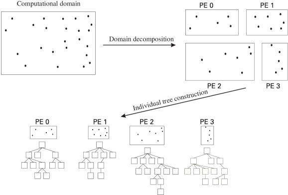
For our N-body/SPH code we have implemented a spatial domain decomposition, using the orthogonal recursive bisection (ORB) algorithm (Dubinski 1996). In the first step, a split is found along one spatial direction, e.g. the x-axis, and the collection of processors is grouped into two halves, one for each side of the split. These processors then exchange particles such that they end up hosting only particles lying on their side of the split. In the simplest possible approach, the position of the split is chosen such that there are an equal number of particles on both sides. However, for an efficient simulation code the split should try to balance the work done in the force computation on the two sides. This aspect will be discussed further below.

In a second step, each group of processors finds a new split along a different spatial axis, e.g. the y-axis. This splitting process is repeated recursively until the final groups consist of just one processor, which then hosts a rectangular piece of the computational volume. Note that this algorithm constrains the number of processors that may be used to a power of two. Other algorithms for the domain decomposition, for example Voronoi tessellations (Yahagi et al. 1999), are free of this restriction.

A two-dimensional schematic illustration of the ORB is shown in Figure 2. Each processor can construct a local BH tree for its domain, and this tree may be used to compute the force exerted by the processors’ particles on arbitrary test particles in space.

6.2 Parallel computation of the gravitational force

GADGET’s algorithm for parallel force computation differs from that of Dubinski (1996), who introduced the notion of locally essential trees. These are trees that are sufficiently detailed to allow the full force computation for any particle local to a processor, without further need for information from other processors. The locally essential trees can be constructed from the local trees by pruning and exporting parts of these trees to other processors, and attaching these parts as new branches to the local trees. To determine which parts of the trees need to be exported, special tree walks are required.

A difficulty with this technique occurs in the context of dynamic tree updates. While the additional time required to promote local trees to locally essential trees should not be an issue for an integration scheme with a global timestep, it can become a significant source of overhead in individual timestep schemes. Here, often only one per cent or less of all particles require a force update at one of the (small) system timesteps. Even if a dynamic tree update scheme is used to avoid having to reconstruct the full tree every timestep, the locally essential trees are still confronted with subtle synchronization issues for the nodes and particles that have been imported from other processor domains. Imported particles in particular may have received force computations since the last ‘full’ reconstruction of the locally essential tree occurred, and hence need to be re-imported. The local domain will also lack sufficient information to be able to update imported nodes on its own if this is needed. So some additional communication needs to occur to properly synchronize the locally essential trees on each timestep. ‘On-demand’ schemes, involving asynchronous communication, may be the best way to accomplish this in practice, but they will still add some overhead and are probably quite complicated to implement. Also note that the construction of locally essential trees depends on the opening criterion. If the latter is not purely geometric but depends on the particle for which the force is desired, it can be difficult to generate a fully sufficient locally essential tree. For these reasons we chose a different parallelization scheme that scales linearly with the number of particles that need a force computation.

Our strategy starts from the observation that each of the local processor trees is able to provide the force exerted by its particles for any location in space. The full force might thus be obtained by adding up all the partial forces from the local trees. As long as the number of these trees is less than the number of typical particle-node interactions, this computational scheme is practically not more expensive than a tree walk of the corresponding locally essential tree.

A force computation therefore requires a communication of the desired coordinates to all processors. These then walk their local trees, and send partial forces back to the original processor that sent out the corresponding coordinate. The total force is then obtained by summing up the incoming contributions.

In practice, a force computation for a single particle would be badly imbalanced in work in such a scheme, since some of the processors could stop their tree walk already at the root node, while others would have to evaluate several hundred particle-node interactions. However, the time integration scheme advances at a given timestep always a group of $M$ particles of size about 0.5-5 per cent of the total number of particles. This group represents a representative mix of the various clustering states of matter in the simulation. Each processor contributes some of its particle positions to this mix, but the total list of coordinates is the same for all processors. If the domain decomposition is done well, one can arrange that the cumulative time to walk the local tree for all coordinates in this list is the same for all processors, resulting in good work-load balance. In the time integration scheme outlined above, the size $M$ of the group of active particles is always roughly the same from step to step, and it also represents always the same statistical mix of particles and work requirements. This means that the same domain decomposition is appropriate for each of a series of consecutive steps. On the other hand, in a block step scheme with binary hierarchy, a step where all particles are synchronized may be followed by a step where only a very small fraction of particles are active. In general, one cannot expect that the same domain decomposition will balance the work for both of these steps.

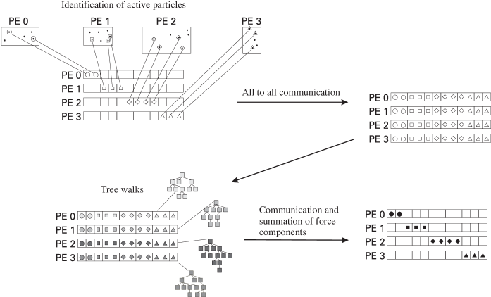
Our force computation scheme proceeds therefore as sketched schematically in Figure 3. Each processor identifies the particles that are to be advanced in the current timestep, and puts their coordinates in a communication buffer. Next, an all-to-all communication phase is used to establish the same list of coordinates on all processors. This communication is done in a collective fashion: For $N_{\rm p}$ processors, the communication involves $N_{\rm p}-1$ cycles. In each cycle, the processors are arranged in $N_{\rm p}/2$ pairs. Each pair exchanges their original list of active coordinates. While the amount of data that needs to be communicated scales as ${\cal O}[M(N_{\rm p}-1)]\simeq{\cal O}(MN_{\rm p})$, the wall-clock time required scales only as ${\cal O}(M+c\,N_{\rm p})$ because the communication is done fully in parallel. The term $c\,N_{\rm p}$ describes losses due to message latency and overhead due to the message envelopes. In practice, additional losses can occur on certain network topologies due to message collisions, or if the particle numbers contributed to $M$ by the individual processors are significantly different, resulting in communication imbalance. On the T3E, the communication bandwidth is large enough that only a very small fraction of the overall simulation time is spent in this phase, even if processor partitions as large as 512 are used. On Beowulf-class networks of workstations, we find that typically less than about 10-20% of the time is lost due to communication overhead if the computers are connected by a switched network with a speed of $100\,{\rm Mbit\,s^{-1}}$.

In the next step, all processors walk their local trees and replace the coordinates with the corresponding force contribution. Note that this is the most time-consuming step of a collisionless simulation (as it should be), hence work-load balancing is most crucial here. After that, the force contributions are communicated in a similar way as above between the processor pairs. The processor that hosted a particular coordinate adds up the incoming force contributions and finally ends up with the full force for that location. These forces can then be used to advance its locally active particles, and to determine new timesteps for them. In these phases of the N-body algorithm, as well as in the tree construction, no further information from other processors is required.

6.3 Work-load balancing

Due to the high communication bandwidth of parallel supercomputers like the T3E or the SP/2, the time required for force computation is dominated by the tree walks, and this is also the dominating part of the simulation as a whole. It is therefore important that this part of the computation parallelizes well. In the context of our parallelization scheme, this means that the domain decomposition should be done such that the time spent in the tree walks of each step is the same for all processors.

It is helpful to note, that the list of coordinates for the tree walks is independent of the domain decomposition. We can then think of each patch of space, represented by its particles, to cause some cost in the tree-walk process. A good measure for this cost is the number of particle-node interactions originating from this region of space. To balance the work, the domain decomposition should therefore try to make this cost equal on the two sides of each domain split.

In practice, we try to reach this goal by letting each tree-node carry a counter for the number of node-particle interactions it participated in since the last domain decomposition occurred. Before a new domain decomposition starts, we then assign this cost to individual particles in order to obtain a weight factor reflecting the cost they on average incur in the gravity computation. For this purpose, we walk the tree backwards from a leaf (i.e. a single particle) to the root node. In this walk, the particle collects its total cost by adding up its share of the cost from all its parent nodes. The computation of these cost factors differs somewhat from the method of Dubinski (1996), but the general idea of such a work-load balancing scheme is similar.

Note that an optimum work-load balance can often result in substantial memory imbalance. Tree-codes consume plenty of memory, so that the feasible problem size can become memory rather than CPU-time limited. For example, a single node with 128 Mbyte on the Garching T3E is already filled to roughly 65 per cent with 4.0$\times 10^{5}$ particles by the present code, including all memory for the tree structures, and the time integration scheme. In this example, the remaining free memory can already be insufficient to allow an optimum work-load balance in strongly clustered simulations. Unfortunately, such a situation is not untypical in practice, since one usually strives for large $N$ in N-body work, so one is always tempted to fill up most of the available memory with particles, without leaving much room to balance the work-load. Of course, GADGET can only try to balance the work within the constraints set by the available memory. The code will also strictly observe a memory limit in all intermediate steps of the domain decomposition, because some machines (e.g. T3E) do not have virtual memory.

6.4 Parallelization of SPH

Hydrodynamics can be seen as a more natural candidate for parallelization than gravity, because it is a local interaction. In contrast to this, the gravitational N-body problem has the unpleasant property that at all times each particle interacts with every other particle, making gravity intrinsically difficult to parallelize on distributed memory machines.

It therefore comes as no large surprise that the parallelization of SPH can be handled by invoking the same strategy we employed for the gravitational part, with only minor adjustments that take into account that most SPH particles (those entirely ‘inside’ a local domain) do not rely on information from other processors.

In particular, as in the purely gravitational case, we do not import neighbouring particles from other processors. Rather, we export the particle coordinates (and other information, if needed) to other processors, which then deliver partial hydrodynamical forces or partial densities contributed by their particle population. For example, the density computation of SPH can be handled in much the same way as that of the gravitational forces. In a collective communication, the processors establish a common list of all coordinates of active particles together with their smoothing lengths. Each processor then computes partial densities by finding those of its particles that lie within each smoothing region, and by doing the usual kernel weighting for them. These partial densities are then delivered back to the processor that holds the particle corresponding to a certain entry in the list of active coordinates. This processor then adds up the partial contributions, and obtains the full density estimate for the active particle.

The locality of the SPH interactions brings an important simplification to this scheme. If the smoothing region of a particle lies entirely inside a local domain, the particle coordinate does not have to be exported at all, allowing a large reduction in the length of the common list of coordinates each processor has to work on, and reducing the necessary amount of communication involved by a large factor.

In the first phase of the SPH computation, we find in this way the density and the total number of neighbours inside the smoothing length, and we evaluate velocity divergence and curl. In the second phase, the hydrodynamical forces are then evaluated in an analogous fashion.

Notice that the computational cost and the communication overhead of this scheme again scale linearly with the number $M$ of active particles, a feature that is essential for good adaptivity of the code. We also note that in the second phase of the SPH computation, the particles ‘see’ the updated density values automatically. When SPH particles themselves are imported to form a locally essential SPH-domain, they have to be exchanged a second time if they are active particles themselves in order to have correctly updated density values for the hydrodynamical force computation (Davé et al. 1997).

An interesting complication arises when the domain decomposition is not repeated every timestep. In practice this means that the boundaries of a domain may become ‘diffuse’ when some particles start to move out of the boundaries of the original domain. If the spatial region that we classified as interior of a domain is not adjusted, we then risk missing interactions because we might not export a particle that starts to interact with a particle that has entered the local domain boundaries, but is still hosted by another processor. Note that our method to update the neighbour-tree on each single timestep already guarantees that the correct neighbouring particles are always found on a local processor – if such a search is conducted at all. So in the case of soft domain boundaries we only need to make sure that all those particles are really exported that can possibly interact with particles on other processors.

Figure 4: NFW density profiles used in the test of time integration criteria. The solid line gives the shape of the normal (unsoftened) NFW profile, dashed lines are softened according to $\epsilon=0.0004$, 0.004, and 0.04, respectively (see equation 66).

We achieve this by ‘shrinking’ the interior of the local domain. During the neighbour-tree update, we find the maximum spatial extension of all SPH particles on the local domain. These rectangular regions are then gathered from all other processors, and cut with the local extension. If an overlap occurs the local ‘interior’ is reduced accordingly, thereby resulting in a region that is guaranteed to be free of any particle lying on another processor. In this way, the SPH algorithm will produce correct results, even if the domain decomposition is repeated only rarely, or never again. In the case of periodic boundaries, special care has to be taken in treating cuts of the current interior with periodic translations of the other domain extensions.

7 Results and tests

7.1 Tests of timestep criteria

Orbit integration in the collisionless systems of cosmological simulations is much less challenging than in highly non-linear systems like star clusters. As a consequence, all the simple timestep criteria discussed in Section 5.1 are capable of producing accurate results for sufficiently small settings of their tolerance parameters. However, some of these criteria may require a substantially higher computational effort to achieve a desired level of integration accuracy than others, and the systematic deviations under conditions of coarse timestepping may be more severe for certain criteria than for others.

In order to investigate this issue, we have followed the orbits of the particle distribution of a typical NFW-halo (Navarro et al. 1996, 1997) for one Hubble time. The initial radial particle distribution and the initial velocity distribution were taken from a halo of circular velocity $1350\,{\rm km\,s^{-1}}$ identified in a cosmological N-body simulation and well fit by the NFW profile. However, we now evolved the particle distribution using a fixed softened potential, corresponding to the mass profile

$$\rho(r)=\frac{\delta_{c}\rho_{\rm crit.}}{\left(\frac{r}{r_{s}}+\epsilon\right)\left(1+\frac{r}{r_{s}}\right)^{2}},$$ (66)

fitted to the initial particle distribution. We use a static potential in order to be able to isolate properties of the time integration only. As a side-effect this also allows a quick integration of all orbits for a Hubble time, and the analytic formulae for the density and potential can also be used to check energy conservation for each of the particles individually. Note that we introduced a softening parameter $\epsilon$ in the profile which is not present in the normal NFW parameterization. The halo had concentration $c=8$ with $r_{s}=170\,h^{-1}{\rm kpc}$, and contained about 140000 particles inside the virial radius. We followed the orbits of all particles inside a sphere of radius $3000\,h^{-1}{\rm kpc}$ around the halo center (about 200000 in total) using GADGET’s integration scheme for single particles in haloes of three different softening lengths, $\epsilon=0.0004$, 0.004, and 0.04. The corresponding density profiles are plotted in Figure 4.

Figure 5: Radii enclosing a fixed mass ($7.1\times 10^{-5}$, $3.6\times 10^{-4}$, $1.8\times 10^{-3}$, $7.1\times 10^{-3}$, $3.6\times 10^{-2}$, $2.1\times 10^{-1}$, and $7.1\times 10^{-1}$ in units of the virial mass) after integrating the particle population of a NFW halo in a fixed potential for one Hubble time with various timestep criteria. Solid lines are for fixed timesteps for all particles, dashed lines for timesteps based on $\Delta t\propto|{\bf a}|^{-1}$, dotted lines for $\Delta t\propto|{\bf a}|^{-1/2}$, and dot-dashed for timesteps based on the local dynamical time, i.e. $\Delta t\propto\rho^{-1/2}$. The three panels are for softened forms of the NFW potential according to equation (66). Note that the fluctuations of the lowest radial shell are caused by the low sampling of the halo in the core and are not significant. The horizontal axis gives the mean number of force evaluation per particle required to advance the particle set for one Hubble time.

In Figure 5, we give the radii of shells enclosing fixed numbers of particles as a function of the mean number of force evaluations necessary to carry out the integration for one Hubble time. The Figure thus shows the convergence of these radii when more and more computational effort is spent.

The results show several interesting trends. In general, for poor integration accuracy (on the left), all radii are much larger than the converged values, i.e. the density profile shows severe signs of relaxation even at large distances from the center. When an integrator with fixed timestep is used (solid lines), the radii decrease monotonically when more force evaluations, i.e. smaller timesteps, are taken, until convergence to asymptotic values is reached. The other timestep criteria converge to these asymptotic values much more quickly. Also, for small softening values, the timestep criterion $\Delta t\propto|{\bf a}|^{-1}$ (dashed lines) performs noticeably better than the one with $t\propto|{\bf a}|^{-1/2}$ (dotted lines), i.e. it is usually closer to the converged values at a given computational cost. On the other hand, the criterion based on the local dynamical time (dot-dashed lines) does clearly the best job. It stays close to the converged values even at a very low number of timesteps.

This impression is corroborated when the softening length is increased. The timestep based on the local dynamical time performs better than the other two simple criteria, and the fixed timestep. Interestingly, the criteria based on the acceleration develop a non-monotonic behaviour when the potential is softened. Already at $\epsilon=0.004$ this is visible at the three lowest radii, but more clearly so for $\epsilon=0.04$. Before the radii increase when poorer integration settings are chosen, they actually first decrease. There is thus a regime where both of these criteria can lead to a net loss of energy for particles close to the shallow core induced by the softening, thereby steepening it. We think that this is related to the fact that the timesteps actually increase towards the center for the criteria (37) and (38) as soon as the logarithmic slope of the density profile becomes shallower than -1. On the other hand, the density increases monotonically towards the center, and hence a timestep based the local dynamical time will decrease. If one uses the local velocity dispersion in the criterion (37), a better behaviour can be obtained, because the velocity dispersion declines towards the center in the core region of dark matter haloes. However, this is not enough to completely suppress non-monotonic behaviour, as we have found in further sets of test calculations.

We thus think that in particular for the cores of large haloes the local dynamical time provides the best of the timestep criteria tested. It leads to hardly any secular evolution of the density profile down to rather coarse timestepping. On the other hand, as Quinn et al. (1997) have pointed out, estimating the density in a real simulation poses additional problems. Since kernel estimates are carried out over a number of neighbours, the density in small haloes can be underestimated, resulting in ‘evaporation’ of haloes. These haloes are better treated with a criterion based on local acceleration, which is much more accurately known in this case.

We thus think that a conservative and accurate way to choose timesteps in cosmological simulations is obtained by taking the minimum of (37) and (39). This requires a computation of the local matter density and local velocity dispersion of collisionless material. Both of these quantities can be obtained for the dark matter just as it is done for the SPH particles. Of course, this requires additional work in order to find neighbours and to do the appropriate summations and kernel estimates, which is, however, typically not more than $\sim 30$% of the cost the gravitational force computation. However, as Figure 5 shows, this is in general worth investing, because the alternative timestep criteria require more timesteps, and hence larger computational cost, by a larger factor in order to achieve the same accuracy.

Figure 6: Cumulative distribution of the relative force error obtained as a function of the tolerance parameter for three opening criteria, and for two different particle distribution. The panels in the left column show results for the particle distribution in the initial conditions of a $32^{3}$ simulation at $z=25$, while the panels on the right give the force errors for the evolved and clustered distribution at $z=0$.

Figure 7: Computational efficiency of three different cell-opening criteria, parameterized by their tolerance parameters. The horizontal axes is proportional to the computational cost, and the vertical axes gives the 95% percentile of the cumulative distribution of relative force errors in a $32^{3}$ cosmological simulation. The left panel shows results for the initial conditions at $z=25$, the right panel for the clustered distribution at redshift $z=0$.

7.2 Force accuracy and opening criterion

In Section 3.3, we have outlined that standard values of the BH-opening criterion can result in very high force errors for the initial conditions of cosmological N-body simulations. Here, the density field is very close to being homogeneous, so that small peculiar accelerations arise from a cancellation of relatively large partial forces. We now investigate this problem further using a cosmological simulation with $32^{3}$ particles in a periodic box. We consider the particle distribution of the initial conditions at redshift $z=25$, and the clustered one of the evolved simulation at $z=0$. Romeel Davé has kindly made these particle dumps available to us, together with exact forces he calculated for all particles with a direct summation technique, properly including the periodic images of the particles. In the following we will compare his forces (which we take to be the exact result) to the ones computed by the parallel version of GADGET using two processors on a Linux PC.

We first examine the distribution of the relative force error as a function of the tolerance parameter used in the two different cell-opening criteria (8) and (18). These results are shown in Figure 6, where we also contrast these distributions with the ones obtained with an optimum cell-opening strategy. The latter may be operationally defined as follows:

Any complete tree walk results in an interaction list that contains a number of internal tree nodes (whose multipole expansions are used) and a number of single particles (which give rise to exact partial forces). Obviously, the shortest possible interaction list is that of just one entry, the root node of the tree itself. Suppose we start with this interaction list, and then open always the one node of the current interaction list that gives rise to the largest absolute force error. This is the node with the largest difference between multipole expansion and exact force, as resulting from direct summation over all the particles represented by the node. With such an opening strategy, the shortest possible interaction list can be found for any desired level of accuracy. The latter may be set by requiring that the largest force error of any node in the interaction list has fallen below a fraction $\delta|{\bf a}|$ of the true force field.

Of course, this optimum strategy is not practical in a real simulation, after all it requires the knowledge of all the exact forces for all internal nodes of the tree. If these were known, we wouldn’t have to bother with trees to begin with. However, it is very interesting to find out what such a fiducial optimum opening strategy would ultimately deliver. Any other analytic or heuristic cell-opening criterion is bound to be worse. Knowing how much worse such criteria are will thus inform us about the maximum performance improvement possible by adopting alternative cell-opening criteria. We therefore computed for each particle the exact direct summation forces exerted by each of the internal nodes, hence allowing us to perform an optimum tree walk in the above way. The resulting cumulative error distributions as a function of $\delta$ are shown in Figure 6.

Looking at this Figure, it is clear that the BH error distribution has a more pronounced tail of large force errors compared to the opening criterion (18). What is most striking however is that at high redshift the BH force errors can become very large for values of the opening angle $\theta$ that tend to give perfectly acceptable accuracy for a clustered mass distribution. This is clearly caused by its purely geometrical nature, which does not know about the smallness of the net forces, and thus does not invest sufficient effort to evaluate partial forces to high enough accuracy.

The error distributions alone do not tell yet about the computational efficiency of the cell-opening strategies. To assess these, we define the error for a given cell-opening criterion as the 95% percentile of the error distribution, and we plot this versus the mean length of the interaction list per particle. This length is essentially linearly related to the computational cost of the force evaluation.

In Figure 7, we compare the performance of the cell-opening criteria in this way. At high redshift, we see that the large errors of the BH criterion are mainly caused because the mean length of the interaction list remains small and does not adapt to the more demanding requirements of the force computation in this regime. Our ‘new’ cell-opening criterion does much better in this respect; its errors remain well controlled without having to adjust the tolerance parameter.

Another advantage of the new criterion is that it is in fact more efficient than the BH criterion, i.e. it achieves higher force accuracy for a given computational expense. As Figure 7 shows, for a clustered particle distribution in a cosmological simulation, the implied saving can easily reach a factor 2-3, speeding up the simulation by the same factor. Similar performance improvements are obtained for isolated galaxies, as the example in Figure 8 demonstrates. This can be understood as follows: The geometrical BH criterion does not take the dynamical significance of the mass distribution into account. For example, it will invest a large number of cell-particle interactions to compute the force exerted by a large void to a high relative accuracy, while actually this force is of small absolute size, and it would be better to concentrate more on those regions that provide most of the force on the current particle. The new opening criterion follows this latter strategy, improving the force accuracy at a given number of particle-cell interactions.

We note that the improvement obtained by criterion (18) brings us about halfway to what might ultimately be possible with an optimum criterion. It thus appears that there is still room for further improvement of the cell-opening criterion, even though it is clear that the optimum will likely not be reachable in practice.

Figure 8: Force errors for an isolated halo/disk galaxy with the BH-criterion (boxes), and the new opening criterion (triangles). The dark halo of the galaxy is modeled with a NFW profile and is truncated at the virial radius. The plot shows the 90% percentile of the error distribution, i.e. 90% of the particles have force errors below the cited values. The horizontal axes measures the computational expense.

7.3 Colliding disk galaxies

As a test of the performance and accuracy of the integration of collisionless systems, we here consider a pair of merging disk galaxies. Each galaxy has a massive dark halo consisting of 30000 particles, and an embedded stellar disk, represented by 20000 particles. The dark halo is modeled according to the NFW-profile, adiabatically modified by the central exponential disk, which contributes 5% of the total mass. The halo has a circular velocity $v_{200}=160\,{\rm km}\,{\rm s}^{-1}$, a concentration $c=5$, and spin parameter $\lambda=0.05$. The radial exponential scale length of the disk is $R_{\rm d}=4.5\,h^{-1}{\rm kpc}$, while the vertical structure is that of an isothermal sheet with thickness $z_{0}=0.2R_{\rm d}$. The gravitational softening of the halo particles is set to $0.4\,h^{-1}{\rm kpc}$, and that of the disk to $0.1\,h^{-1}{\rm kpc}$.

Initially, the two galaxies are set-up on a parabolic orbit, with separation such that their dark haloes just touch. Both of the galaxies have a prograde orientation, but are inclined with respect to the orbital plane. In fact, the test considered here corresponds exactly to the simulation ‘C1’ computed by Springel (2000), where more information about the construction of the initial conditions can be found (see also Springel & White 1999).

We first consider a run of this model with a set of parameters equal to the coarsest values we would typically employ for a simulation of this kind. For the time integration, we used the parameter $\alpha_{\rm tol}\sigma=25\,{\rm km}\,{\rm s}^{-1}$, and for the force computation with the tree algorithm, the new opening criterion with $\alpha=0.04$. The simulation was then run from $t=0$ to $t=2.8$ in internal units of time (corresponding to $2.85\,h^{-1}{\rm Gyr}$). During this time the galaxies have their first close encounter at around $t\simeq 1.0$, where tidal tails are ejected out of the stellar disks. Due to the braking by dynamical friction, the galaxies eventually fall together for a second time, after which they quickly merge and violently relax to form a single merger remnant. At $t=2.8$, the inner parts of the merger remnant are well relaxed.

This simulation required a total number of 4684 steps and 27795733 force computations, i.e. a computationally equally expensive computation with fixed timesteps could just make 280 full timesteps. The relative error in the total energy was $3.0\times 10^{-3}$, and a Sun Ultrasparc-II workstation (sparcv9 processor, 296 MHz clock speed) did the simulation in 4 hours (using the serial code). The raw force speed was $\sim$2800 force computations per second, older workstations will achieve somewhat smaller values, of course. Also, higher force accuracy settings will slow down the code somewhat.

Figure 9: Spherically averaged density profile of the stellar component in the merger remnant of two colliding disk galaxies. Triangles show the results obtained using our variable timestep integration, while boxes and diamonds are for fixed timestep integrations with $\Delta t=0.01$ ($10\,h^{-1}{\rm Myr}$) and $\Delta t=0.0025$ ($2.5\,h^{-1}{\rm Myr}$), respectively. Note that the simulation using the adaptive timestep is about as expensive as the one with $\Delta t=0.01$. In each case, the center of the remnant was defined as the position of the particle with the minimum gravitational potential.

We now consider a simulation of the same system using a fixed timestep. For $\Delta t=0.01$, the run needs 280 full steps, i.e. it consumes the same amount of CPU time as above. However, in this simulation, the error in the total energy is $2.2\%$, substantially larger than before. There are also differences in the density profile of the merger remnants. In Figure 9, we compare the inner density profile of the simulation with adaptive timesteps (triangles) to the one with a fixed timestep of $\Delta t=0.01$ (boxes). We here show the spherically averaged profile of the stellar component, with the center of the remnants defined as the position of the particle with the minimum gravitational potential. It can be seen that in the innermost $\sim 1\,h^{-1}{\rm kpc}$, the density obtained with the fixed timestep falls short of the adaptive timestep integration.

To get an idea how small the fixed timestep has to be to achieve similar accuracy as with the adaptive timestep, we have simulated this test a second time, with a fixed timesteps of $\Delta t=0.0025$. We also show the corresponding profile (diamonds) in Figure 9. It can be seen that for smaller $\Delta t$, the agreement with the variable timestep result improves. At $\sim 2\times 0.4\,h^{-1}{\rm kpc}$, the softening of the dark matter starts to become important. For agreement down to this scale, the fixed timestep needs to be slightly smaller than $\Delta t=0.0025$, so the overall saving due to the use of individual particle timesteps is at least a factor of $4-5$ in this example.

Figure 10: Time evolution of the thermal, kinetic, potential, and total energy for the collapse of an initially isothermal gas sphere. Solid lines show results for a simulations with 30976 particles, dashed lines are for a 4224 particle run.

7.4 Collapse of a cold gas sphere

The self-gravitating collapse of an initially isothermal, cool gas sphere has been a common test problem of SPH codes (Evrard 1988; Hernquist & Katz 1989; Steinmetz & Müller 1993; Thacker et al. 2000; Carraro et al. 1998, and others). Following these authors, we consider a spherically symmetric gas cloud of total mass $M$, radius $R$, and initial density profile

$$\rho(r)=\frac{M}{2\pi R^{2}}\;\frac{1}{r}.$$ (67)

We take the gas to be of constant temperature initially, with an internal energy per unit mass of

$$u=0.05\,\frac{GM}{R}.$$ (68)

At the start of the simulation, the gas particles are at rest. We obtain their initial coordinates from a distorted regular grid that reproduces the density profile (67), and we use a system of units with $G=M=R=1$.

In Figure 10, we show the evolution of the potential, the thermal, and the kinetic energy of the system from the start of the simulation at $t=0$ to $t=3$. We plot results for two simulations, one with 30976 particles (solid), and one with 4224 particles (dashed). During the central bounce between $t\approx 0.8$ and $t\approx 1.2$ most of the kinetic energy is converted into heat, and a strong shock wave travels outward. Later, the system slowly settles to virial equilibrium.

For these runs $N_{\rm s}$ was set to 40, the gravitational softening to $\epsilon=0.02$, and time integration was controlled by the parameters $\alpha_{\rm tol}\sigma=0.05$ and $\alpha_{\rm cour}=0.1$, resulting in very good energy conservation. The absolute error in the total energy is less than $1.1\times 10^{-3}$ at all times during the simulation, translating to a relative error of 0.23%. Since we use a time integration scheme with individual timesteps of arbitrary size, this small error is reassuring. The total number of small steps taken by the 4224 particle simulation was 3855, with a total of 2192421 force computations, i.e. the equivalent number of ‘full’ timesteps was 519. A Sun Ultrasparc-II workstation needed 2300 seconds for the simulation. The larger 30976 particle run took 10668 steps, with an equivalent of 1086 ‘full’ steps, and 12 hours of CPU time. Note that by reducing the time integration accuracy by a factor of 2, with a corresponding reduction of the CPU time consumption by the same factor, the results do practically not change, however, the maximum error in the energy goes up to 1.2% in this case.

Table 1: Consumption of CPU-time in various parts of the code for a cosmological run from $z=50$ to $z=4.3$. The table gives timings for runs with 4, 8 and 16 processors on the Garching Cray T3E. The computation of the gravitational forces is by far the dominant computational task. We have further split up that time into the actual tree-walk time, the tree-construction time, the time for communication and summation of force contributions, and into the time lost by work-load imbalance. The potential computation is done only once in this test (it can optionally be done in regular intervals to check energy conservation of the code). ‘Miscellaneous’ refers to time spent in advancing and predicting particles, and in managing the binary tree for the timeline. I/O time for writing a snapshot file (groups of processors can write in parallel) is only 1-2 seconds, and therefore not listed here.

	4 processors		8 processors		16 processors
	cumulative time [sec]	relative time	cumulative time [sec]	relative time	cumulative time [sec]	relative time
total	8269.0	100.0 %	4074.0	100.0 %	2887.5	100.0 %
gravity	7574.6	91.6 %	3643.0	89.4 %	2530.3	87.6 %
tree walks	5086.3	61.5 %	2258.4	55.4 %	1322.4	45.8 %
tree construction	1518.4	18.4 %	773.7	19.0%	588.4	20.4 %
communication & summation	24.4	0.3 %	35.4	0.9 %	54.1	1.9 %
work-load imbalance	901.5	10.9 %	535.1	13.1 %	537.4	18.6 %
domain decomposition	209.9	2.5 %	158.1	3.9 %	172.2	6.0 %
potential computation (optional)	46.3	0.2 %	18.1	0.4 %	11.4	0.4 %
miscellaneous	438.3	5.3 %	254.8	6.3 %	173.6	6.0 %

The results of Figure 10 agree very well with those of Steinmetz & Müller (1993), and with Thacker et al. (2000) if we compare to their ‘best’ implementation of artificial viscosity (their version 12). Steinmetz & Müller (1993) have also computed a solution of this problem with a very accurate, one-dimensional, spherically symmetric piecewise parabolic method (PPM). For particle numbers above 10000, our SPH results become very close to the finite difference result. However, even for very small particle numbers, SPH is capable of reproducing the general features of the solution very well. We also expect that a three-dimensional PPM calculation of the collapse would likely require at least the same amount of CPU time as our SPH calculation.

7.5 Performance and scalability of the parallel gravity

We here show a simple test of the performance of the parallel version of the code under conditions relevant for real target applications. For this test, we have used a ‘stripped-down’ version of the initial conditions originally constructed for a high-resolution simulation of a cluster of galaxies. The original set of initial conditions was set-up to follow the cosmological evolution of a large spherical region with comoving radius $70\,h^{-1}{\rm Mpc}$, within a $\Lambda$CDM cosmogony corresponding to $\Omega_{0}=0.3$, $\Omega_{\Lambda}=0.7$, $z_{\rm start}=50$, and $h=0.7$. In the center of the simulation sphere, 2 million high-resolution particles were placed in the somewhat enlarged Lagrangian region of the cluster. The rest of the volume was filled with an extended shell of boundary particles of larger mass and larger softening; they are needed for a proper representation of the gravitational tidal field.

Figure 11: Code performance and scalability for a cosmological integration with vacuum boundaries. The left panel shows the speed of the gravitational force computation as a function of processor number (in particles per second). This is based on the tree walk time alone. In the simulation, additional time is needed for tree construction, work-load imbalance, communication, domain decomposition, prediction of particles, timeline, etc. This reduces the ‘effective’ speed of the code, as shown in the right panel. This effective speed gives the number of particles advanced by one timestep per second. Note that the only significant source of work-load imbalance in the code occurs in the gravity computation, where some small fraction of time is lost when processors idly wait for others to finish their tree-walks.

To keep our test simple, we have cut a centred sphere of comoving radius $12.25\,h^{-1}{\rm Mpc}$ from these initial conditions, and we only simulated the 500000 high-resolution particles with mass $m_{\rm p}=1.36\times 10^{9}h^{-1}{\rm M}_{\odot}$ found within this region. Such a simulation will not be useful for direct scientific analysis because it does not model the tidal field properly. However, this test will show realistic clustering and time-stepping behaviour, and thus allows a reasonable assessment of the expected computational cost and scaling of the full problem.

We have run the test problem with GADGET on the Garching T3E from redshift $z=50$ to redshift $z=4.3$. We repeated the identical run on partitions of size 4, 8, and 16 processors. In this test, we included quadrupole moments in the tree computation, we used a BH opening criterion with $\theta=1.0$, and a gravitational softening length of $15\,h^{-1}{\rm kpc}$.

In Table 1 we list in detail the elapsed wall-clock time for various parts of the code for the three simulations. The dominant sink of CPU time is the computation of gravitational forces for the particles. To advance the test simulation from $z=50$ to $z=4.3$, GADGET needed $30.0\times 10^{6}$ force computations in a total of 3350 timesteps. Note that on average only 1.8% of the particles are advanced in a single timestep. Under these conditions it is challenging to eliminate sources of overhead incurred by the time-stepping and to maintain work-load balancing. GADGET solves this task satisfactorily. If we used a fixed timestep, the work-load balancing would be essentially perfect. Note that the use of our adaptive timestep integrator results in a saving of about a factor of 3-5 compared to a fixed timestep scheme with the same accuracy.

We think that the overall performance of GADGET is good in this test. The raw gravitational speed is high, and the algorithm used to parallelize the force computation scales well, as is seen in the left panel of Figure 11. Note that the force-speed of the $N_{\rm p}=8$ run is even higher than that of the $N_{\rm p}=4$ run. This is because the domain decomposition does exactly one split in the $x$-, $y$-, and $z$-directions in the $N_{\rm p}=8$ case. The domains are then close to cubes, which reduces the depth of the tree and speeds up the tree-walks.

Also, the force communication does not involve a significant communication overhead, and the time spent in miscellaneous tasks of the simulation code scales closely with processor number. Most losses in GADGET occur due to work-load imbalance in the force computation. While we think these losses are acceptable in the above test, one should keep in mind that we here kept the problem size fixed, and just increased the processor number. If we also scale up the problem size, work-load balancing will be significantly easier to achieve, and the efficiency of GADGET will be nearly as high as for small processor number.

Nevertheless, the computational speed of GADGET may seem disappointing when compared with the theoretical peak performance of modern microprocessors. For example, the processors of the T3E used for the timings have a nominal peak performance of 600 MFlops, but GADGET falls far short of reaching this. However, the peak performance can only be reached under the most favourable of circumstances, and typical codes operate in a range where they are a factor of 5-10 slower. GADGET is no exception here. While we think that the code does a reasonable job in avoiding unnecessary floating point operations, there is certainly room for further tuning measures, including processor-specific ones which haven’t been tried at all so far. Also note that our algorithm of individual tree walks produces essentially random access of memory locations, a situation that could hardly be worse for the cache pipeline of current microprocessors.

7.6 Parallel SPH in a periodic volume

As a further test of the scaling and performance of the parallel version of GADGET in typical cosmological applications we consider a simulation of structure formation in a periodic box of size $(50h^{-1}{\rm Mpc})^{3}$, including adiabatic gas physics. We use $32^{3}$ dark matter particles, and $32^{3}$ SPH particles in a $\Lambda$CDM cosmology with $\Omega_{0}=0.3$, $\Omega_{\Lambda}=0.7$ and $h=0.7$, normalized to $\sigma_{8}=0.9$. For simplicity, initial conditions are constructed by displacing the particles from a grid, with the SPH particles placed on top of the dark matter particles.

Figure 12: Speed of the code in a gasdynamical simulation of a periodic $\Lambda$CDM universe, run from $z=10$ to $z=1$, as a function of the number of T3E processors employed. The top panel shows the speed of the gravitational force computation (including tree construction times). We define the speed here as the number of force computations per elapsed wall-clock time. The middle panel gives the speed in the computation of hydrodynamical forces, while the bottom panel shows the resulting overall code speed in terms of particles advanced by one timestep per second. This effective code speed includes all other code overhead, which is less than 5% of the total cpu time in all runs.

We have evolved these initial conditions from $z=10$ to $z=1$, using 2, 4, 8, 16, and 32 processors on the Cray T3E in Garching. The final particle distributions of all these runs are in excellent agreement with each other.

In the bottom panel of Figure 12, we show the code speed as a function of the number of processors employed. We here define the speed as the total number of force computations divided by the total elapsed wall-clock time during this test. Note that the scaling of the code is almost perfectly linear in this example, even better than for the set-up used in the previous section. In fact, this is largely caused by the simpler geometry of the periodic box as compared to the spherical volume used earlier. The very absence of such boundary effects makes the periodic box easier to domain-decompose, and to work-balance.

The top and middle panels of Figure 12 show the speed of the gravitational force computation and that of the SPH part separately. What we find encouraging is that the SPH algorithm scales really very well, which is promising for future large-scale applications.

It is interesting that in this test (where $N_{\rm s}=40$ SPH neighbours have been used) the hydrodynamical part actually consumes only $\sim 25\%$ of the overall CPU time. Partly this is due to the slower gravitational speed in this test compared to the results shown in Figure 11, which in turn is caused by the Ewald summation needed to treat the periodic boundary conditions, and by longer interaction lists in the present test (we here used our new opening criterion). Also note that only half of the particles in this simulation are SPH particles.

We remark that the gravitational force computation will usually be more expensive at higher redshift than at lower redshift, while the SPH part does not have such a dependence. The fraction of time consumed by the SPH part thus tends to increase when the material becomes more clustered. In dissipative simulations one will typically form clumps of cold gas with very high density - objects that we think will form stars and turn into galaxies. Such cold knots of gas can slow down the computation substantially, because they require small hydrodynamical timesteps, and if a lower spatial resolution cut-off for SPH is imposed, the hydrodynamical smoothing may start to involve more neighbours than $N_{\rm s}$.

8 Discussion

We have presented the numerical algorithms of our code GADGET, designed as a flexible tool to study a wide range of problems in cosmology. Typical applications of GADGET can include interacting and colliding galaxies, star formation and feedback in the interstellar medium, formation of clusters of galaxies, or the formation of large-scale structure in the universe.

In fact, GADGET has already been used successfully in all of these areas. Using our code, Springel & White (1999) have studied the formation of tidal tails in colliding galaxies, and Springel (2000) has modeled star formation and feedback in isolated and colliding gas-rich spirals. For these simulations, the serial version of the code was employed, both with and without support by the GRAPE special-purpose hardware.

The parallel version of GADGET has been used to compute high-resolution N-body simulations of clusters of galaxies (Springel 1999; Springel et al. 2000; Yoshida et al. 2000a, b). In the largest simulation of this kind, 69 million particles have been employed, with 20 million of them ending up in the virialized region of a single object. The particle mass in the high-resolution zone was just $\sim 10^{-10}$ of the total simulated mass, and the gravitational softening length was $0.7\,h^{-1}{\rm kpc}$ in a simulation volume of diameter $140\,h^{-1}{\rm Mpc}$, translating to an impressive spatial dynamic range of $2\times 10^{5}$ in three dimensions.

We have also successfully employed GADGET for two ‘constrained-realization’ (CR) simulations of the Local Universe (Mathis et al. 2000, in preparation). In these simulations, the observed density field as seen by IRAS galaxies has been used to constrain the phases of the waves of the initial fluctuation spectrum. For each of the two CR simulations, we employed $\sim 75$ million particles in total, with 53 million high-resolution particles of mass $3.6\times 10^{9}h^{-1}{\rm M}_{\odot}$ ($\Lambda$CDM) or $1.2\times 10^{10}h^{-1}{\rm M}_{\odot}$ ($\tau$CDM) in the low-density and critical-density models, respectively.

The main technical features of GADGET are as follows. Gravitational forces are computed with a Barnes & Hut oct-tree, using multipole expansions up to quadrupole order. Periodic boundary conditions can optionally be used and are implemented by means of Ewald summation. The cell-opening criterion may be chosen either as the standard BH-criterion, or a new criterion which we have shown to be computationally more efficient and better suited to cosmological simulations starting at high redshift. As an alternative to the tree-algorithm, the serial code can use the special-purpose hardware GRAPE  both to compute gravitational forces and for the search for SPH neighbours.

In our SPH implementation, the number of smoothing neighbors is kept exactly constant in the serial code, and is allowed to fluctuate in a small band in the parallel code. Force symmetry is achieved by using the kernel averaging technique, and a suitable neighbour searching algorithm is used to guarantee that all interacting pairs of SPH particles are always found. We use a shear-reduced artificial viscosity that has emerged as a good parameterization in recent systematic studies that compared several alternative formulations (Thacker et al. 2000; Lombardi et al. 1999).

Parallelization of the code for massively parallel supercomputers is achieved in an explicit message passing approach, using the MPI standard communication library. The simulation volume is spatially split using a recursive orthogonal bisection, and each of the resulting domains is mapped onto one processor. Dynamic work-load balancing is achieved by measuring the computational expense incurred by each particle, and balancing the sum of these weights in the domain decomposition.

The code allows fully adaptive, individual particle timesteps, both for collisionless particles and for SPH particles. The speed-up obtained by the use of individual timesteps depends on the dynamic range of the time scales present in the problem, and on the relative population of these time scales with particles. For a collisionless cosmological simulation with a gravitational softening length larger than $\sim 30\,h^{-1}{\rm kpc}$ the overall saving is typically a factor of $3-5$. However, if smaller softening lengths are desired, the use of individual particle timesteps results in larger savings. In the hydrodynamical part, the savings can be still larger, especially if dissipative physics is included. In this case, adaptive timesteps may be required to make a simulation feasible to begin with. GADGET can be used to run simulations both in physical and in comoving coordinates. The latter is used for cosmological simulations only. Here, the code employs an integration scheme that can deal with arbitrary cosmological background models, and which is exact in linear theory, i.e. the linear regime can be traversed with maximum efficiency.

GADGET is an intrinsically Lagrangian code. Both the gravity and the hydrodynamical parts impose no restriction on the geometry of the problem, nor any hard limit on the allowable dynamic range. Current and future simulations of structure formation that aim to resolve galaxies in their correct cosmological setting will have to resolve length scales of size $0.1-1\,h^{-1}{\rm kpc}$ in volumes of size $\sim 100\,h^{-1}{\rm Mpc}$. This range of scales is accompanied by a similarly large dynamic range in mass and time scales. Our new code is essentially free to adapt to these scales naturally, and it invests computational work only where it is needed. It is therefore a tool that should be well suited to work on these problems.

Since GADGET is written in standard ANSI-C, and the parallelization for massively parallel supercomputers is achieved with the standard MPI library, the code runs on a large variety of platforms, without requiring any change. Having eliminated the dependence on proprietary compiler software and operating systems we hope that the code will remain usable for the foreseeable future. We release the parallel and the serial version of GADGET publically in the hope that they will be useful for others as a scientific tool and as a basis for further numerical developments.

Appendix: Softened tree nodes

The smoothing kernel we use for SPH calculations is a spline of the form (Monaghan & Lattanzio 1985)

$$W(r;h)=\frac{8}{\pi h^{3}}\left\{\begin{array}[]{ll}1-6\left(\frac{r}{h}\right)^{2}+6\left(\frac{r}{h}\right)^{3},&0\leq\frac{r}{h}\leq\frac{1}{2},\\ 2\left(1-\frac{r}{h}\right)^{3},&\frac{1}{2}<\frac{r}{h}\leq 1,\\ 0,&\frac{r}{h}>1.\end{array}\right.$$ (69)

Note that we define the smoothing kernel on the interval $[0,h]$ and not on $[0,2h]$ as it is frequently done in other SPH calculations.

Figure 13: Comparison of spline-softened (solid) and Plummer-softened (dotted) potential of a point mass with the Newtonian potential (dashed). Here $h=1.0$, and $\epsilon=h/2.8$.

Figure 14: Comparison of spline-softened (solid) and Plummer-softened (dotted) force law with Newton’s law (dashed). Here $h=1.0$, and $\epsilon=h/2.8$.

We derive the spline-softened gravitational force from this kernel by taking the force from a point mass $m$ to be the one resulting from a density distribution $\rho({\bf r})=mW({\bf r};h)$. This leads to a potential

$$\Phi({\bf r})=G\frac{m}{h}W_{2}\left(\frac{r}{h}\right)$$ (70)

with a kernel

$$W_{2}(u)=\left\{\begin{array}[]{ll}\frac{16}{3}u^{2}-\frac{48}{5}u^{4}+\frac{32}{5}u^{5}-\frac{14}{5},&\mbox{$0\leq u<\frac{1}{2}$},\vspace{0.1cm}\\ \frac{1}{15u}+\frac{32}{3}u^{2}-16u^{3}+\frac{48}{5}u^{4}\\ \mbox{\hskip 28.45274pt}-\frac{32}{15}u^{5}-\frac{16}{5},&\mbox{$\frac{1}{2}\leq u<1$},\vspace{0.1cm}\\ -\frac{1}{u},&\mbox{$u\geq 1$}.\\ \end{array}\right.$$ (71)

The multipole expansion of a group of particles is discussed in Section 3.1. It results in a potential and force given by equations (3.1) and (3.1), respectively. The functions appearing in equation (3.1) are defined as

$$g_{1}(y)=\frac{g^{\prime}(y)}{y},$$ (72)

$$g_{2}(y)=\frac{g^{\prime\prime}(y)}{y^{2}}-\frac{g^{\prime}(y)}{y^{3}},$$ (73)

$$g_{3}(y)=\frac{g_{2}^{\prime}(y)}{y},$$ (74)

$$g_{4}(y)=\frac{g_{1}^{\prime}(y)}{y}.$$ (75)

Writing $u=y/h$, the explicit forms of these functions are

$$g_{1}(y)=\frac{1}{h^{3}}\left\{\begin{array}[]{ll}-\frac{32}{3}+\frac{192}{5}u^{2}-32u^{3},&\mbox{$u\leq\frac{1}{2}$},\vspace{0.1cm}\\ \frac{1}{15u^{3}}-\frac{64}{3}+48u\\ \mbox{\hskip 28.45274pt}-\frac{192}{5}u^{2}+\frac{32}{3}u^{3},&\mbox{$\frac{1}{2}<u<1$},\vspace{0.1cm}\\ -\frac{1}{u^{3}},&\mbox{$u>1$,}\end{array}\right.$$ (76)

$$g_{2}(y)=\frac{1}{h^{5}}\left\{\begin{array}[]{ll}\frac{384}{5}-96u,&\mbox{$u\leq\frac{1}{2}$},\vspace{0.1cm}\\ -\frac{384}{5}-\frac{1}{5u^{5}}+\frac{48}{u}+32u,&\mbox{$\frac{1}{2}<u<1$},\vspace{0.1cm}\\ \frac{3}{u^{5}},&\mbox{$u>1$},\end{array}\right.$$ (77)

$$g_{3}(y)=\frac{1}{h^{7}}\left\{\begin{array}[]{ll}-\frac{96}{u},&\mbox{$u\leq\frac{1}{2}$},\vspace{0.1cm}\\ \frac{32}{u}+\frac{1}{u^{7}}-\frac{48}{u^{3}},&\mbox{$\frac{1}{2}<u<1$},\vspace{0.1cm}\\ -\frac{15}{u^{7}},&\mbox{$u>1$},\end{array}\right.$$ (78)

$$g_{4}(y)=\frac{1}{h^{5}}\left\{\begin{array}[]{ll}-\frac{96}{5}(5u-4),&\mbox{$u\leq\frac{1}{2}$},\vspace{0.1cm}\\ \frac{48}{u}-\frac{1}{5u^{5}}-\frac{384}{5}+32u,&\mbox{$\frac{1}{2}<u<1$},\vspace{0.1cm}\\ \frac{3}{u^{5}},&\mbox{$u>1$}.\end{array}\right.$$ (79)

In Figures 13 and 14, we show the spline-softened and Plummer-softened force and potential of a point mass. For a given spline softening length $h$, we define the ‘equivalent’ Plummer softening length as $\epsilon=h/2.8$. For this choice, the minimum of the potential at $u=0$ has the same depth.

References

- Aarseth (1963) Aarseth S. J., 1963, MNRAS, 126, 223
- Aarseth et al. (1979) Aarseth S. J., Turner E. L., Gott J. R., 1979, ApJ, 228, 664
- Appel (1981) Appel A. W., 1981, Undergraduate Thesis, Princeton University
- Appel (1985) Appel A. W., 1985, SIAM, J. Sci. Stat. Comp, 6, 85
- Athanassoula et al. (1998) Athanassoula E., Bosma A., Lambert J. C., Makino J., 1998, MNRAS, 293, 369
- Athanassoula et al. (2000) Athanassoula E., Fady E., Lambert J. C., Bosma A., 2000, MNRAS, 314, 475
- Bagla (1999) Bagla J. S., 1999, preprint, astro-ph/9911025
- Balsara (1995) Balsara D. W., 1995, J. Comp. Phys., 121, 357
- Barnes (1986) Barnes J., 1986, in The Use of Supercomputers in Stellar Dynamics, edited by P. Hut, S. L. J. McMillan, 175, Springer, New York
- Barnes & Hut (1986) Barnes J., Hut P., 1986, Nature, 324, 446
- Barnes (1990) Barnes J. E., 1990, J. Comp. Phys., 87, 161
- Barnes & Hut (1989) Barnes J. E., Hut P., 1989, ApJS, 70, 389
- Bertschinger & Gelb (1991) Bertschinger E., Gelb J. M., 1991, Computers in Physics, 5, 164
- Bode et al. (2000) Bode P., Ostriker J. P., Xu G., 2000, ApJS, 128, 561
- Brieu et al. (1995) Brieu P. P., Summers F. J., Ostriker J. P., 1995, ApJ, 453, 566
- Carraro et al. (1998) Carraro G., Lia C., Chiosi C., 1998, MNRAS, 297, 1021
- Couchman (1991) Couchman H. M. P., 1991, ApJ, 368, 23
- Couchman et al. (1995) Couchman H. M. P., Thomas P., Pearce F., 1995, ApJ, 452, 797
- Davé et al. (1997) Davé R., Dubinski J., Hernquist L., 1997, New Astronomy, 2, 277
- Dikaiakos & Stadel (1996) Dikaiakos M. D., Stadel J., 1996, ICS conference proceedings
- Dubinski (1996) Dubinski J., 1996, New Astronomy, 1, 133
- Dubinski et al. (1996) Dubinski J., Mihos J. C., Hernquist L., 1996, ApJ, 462, 576
- Eastwood & Hockney (1974) Eastwood J. W., Hockney R. W., 1974, J. Comp. Phys., 16, 342
- Ebisuzaki et al. (1993) Ebisuzaki T., Makino J., Fukushige T., et al., 1993, PASJ, 45, 269
- Efstathiou et al. (1985) Efstathiou G., Davis M., Frenk C. S., White S. D. M., 1985, ApJS, 57, 241
- Evrard (1988) Evrard A. E., 1988, MNRAS, 235, 911
- Frenk et al. (1999) Frenk C. S., White S. D. M., Bode P., et al., 1999, ApJ, 525, 554
- Fukushige et al. (1991) Fukushige T., Ito T., Makino J., Ebisuzaki T., Sugimoto D., Umemura M., 1991, PASJ, 43, 841
- Fukushige et al. (1996) Fukushige T., Taiji M., Makino J., Ebisuzaki T., Sugimoto D., 1996, ApJ, 468, 51
- Gingold & Monaghan (1977) Gingold R. A., Monaghan J. J., 1977, MNRAS, 181, 375
- Greengard & Rokhlin (1987) Greengard L., Rokhlin V., 1987, J. Comp. Phys., 73, 325
- Groom (1997) Groom W., 1997, Ph.D. thesis, University of Cambridge
- Hernquist et al. (1991) Hernquist L., Bouchet F. R., Suto Y., 1991, ApJS, 75, 231
- Hernquist & Katz (1989) Hernquist L., Katz N., 1989, ApJ, 70, 419
- Hiotelis & Voglis (1991) Hiotelis N., Voglis N., 1991, A&A, 243, 333
- Hockney & Eastwood (1981) Hockney R. W., Eastwood J. W., 1981, Computer Simulation Using Particles, McGraw-Hill, New Work
- Hohl (1978) Hohl F., 1978, ApJ, 83, 768
- Holmberg (1941) Holmberg E., 1941, ApJ, 94, 385
- Hultman & Källander (1997) Hultman J., Källander D., 1997, A&A, 324, 534
- Hut & Makino (1999) Hut P., Makino J., 1999, Science, 283, 501
- Hut et al. (1995) Hut P., Makino J., McMillan S., 1995, ApJ, 443, 93
- Ito et al. (1991) Ito T., Ebisuzaki T., Makino J., Sugimoto D., 1991, PASJ, 43, 547
- Jernigan & Porter (1989) Jernigan J. G., Porter D. H., 1989, ApJS, 71, 871
- Kang et al. (1994) Kang H., Ostriker J. P., Cen R., et al., 1994, ApJ, 430, 83
- Katz & Gunn (1991) Katz N., Gunn J. E., 1991, ApJ, 377, 365
- Katz et al. (1996) Katz N., Weinberg D. H., Hernquist L., 1996, ApJS, 105, 19
- Kawai et al. (2000) Kawai A., Fukushige T., Makino J., Taiji M., 2000, PASJ, 52, 659
- Klein et al. (1998) Klein R. I., Fisher R. T., McKee C. F., Truelove J. K., 1998, in Proceedings of the International Conference on Numerical Astrophysics 1998 (NAP98), edited by S. M. Miyama, K. Tomisaka, T. Hanawa, p. 131, Kluwer Academic, Boston, Mass.
- Kravtsov et al. (1997) Kravtsov A. V., Klypin A. A., Khokhlov A. M. J., 1997, ApJS, 111, 73
- Lia & Carraro (2000) Lia C., Carraro G., 2000, MNRAS, 314, 145
- Lombardi et al. (1999) Lombardi J. C., Sills A., Rasio F. A., Shapiro S. L., 1999, J. of Comp. Phys., 152, 687
- Lucy (1977) Lucy L. B., 1977, AJ, 82, 1013
- MacFarland et al. (1998) MacFarland T., Couchman H. M. P., Pearce F. R., Pichlmeier J., 1998, New Astronomy, 3, 687
- Makino (1990) Makino J., 1990, PASJ, 42, 717
- Makino (1991a) Makino J., 1991a, PASJ, 43, 621
- Makino (1991b) Makino J., 1991b, ApJ, 369, 200
- Makino (2000) Makino J., 2000, in Dynamics of Star Clusters and the Milky Way, edited by S. Deiters, B. Fuchs, A. Just, R. Spurzem, R. Wielen, astro-ph/0007084
- Makino & Aarseth (1992) Makino J., Aarseth S. J., 1992, PASJ, 44, 141
- Makino & Funato (1993) Makino J., Funato Y., 1993, PASJ, 45, 279
- Makino & Hut (1989) Makino J., Hut P., 1989, Computer Physics Reports, 9, 199
- Makino et al. (1997) Makino J., Taiji M., Ebisuzaki T., Sugimoto D., 1997, ApJ, 480, 432
- McMillan & Aarseth (1993) McMillan S. L. W., Aarseth S. J., 1993, ApJ, 414, 200
- Monaghan (1992) Monaghan J. J., 1992, Ann. Rev. Astron. Astrophys., 30, 543
- Monaghan & Gingold (1983) Monaghan J. J., Gingold R. A., 1983, J. Comp. Phys., 52, 374
- Monaghan & Lattanzio (1985) Monaghan J. J., Lattanzio J. C., 1985, A&A, 149, 135
- Navarro et al. (1996) Navarro J. F., Frenk C. S., White S. D. M., 1996, ApJ, 462, 563
- Navarro et al. (1997) Navarro J. F., Frenk C. S., White S. D. M., 1997, ApJ, 490, 493
- Navarro & White (1993) Navarro J. F., White S. D. M., 1993, MNRAS, 265, 271
- Nelson & Papaloizou (1994) Nelson R. P., Papaloizou J. C. B., 1994, MNRAS, 270, 1
- Norman & Bryan (1998) Norman M. L., Bryan G. L., 1998, in Proceedings of the International Conference on Numerical Astrophysics 1998 (NAP98), edited by S. M. Miyama, K. Tomisaka, T. Hanawa, p. 19, Kluwer Academic, Boston, Mass.
- Okumura et al. (1993) Okumura S. K., Makino J., Ebisuzaki T., et al., 1993, PASJ, 45, 329
- Pacheco (1997) Pacheco P. S., 1997, Parallel Programming with MPI, Morgan Kaufmann Publishers, San Francisco
- Pearce & Couchman (1997) Pearce F. R., Couchman H. M. P., 1997, New Astronomy, 2, 411
- Peebles (1970) Peebles P. J. E., 1970, Astron. J., 75, 13
- Press (1986) Press W. H., 1986, in The Use of Supercomputers in Stellar Dynamics, edited by P. Hut, S. McMillan, 184, Springer-Verlag, Berlin Heidelberg New York
- Press & Schechter (1974) Press W. H., Schechter P., 1974, ApJ, 187, 425
- Press et al. (1995) Press W. H., Teukolsky S. A., Vetterling W. T., Flannery B. P., 1995, Numerical recipies in C, Cambridge University Press, Cambridge
- Quinn et al. (1997) Quinn T., Katz N., Stadel J., Lake G., 1997, preprint, astro-ph/9710043
- Romeo (1998) Romeo A. B., 1998, A&A, 335, 922
- Salmon & Warren (1994) Salmon J. K., Warren M. S., 1994, J. Comp. Phys., 111, 136
- Snir et al. (1995) Snir M., Otto S. W., Huss-Lederman S., Walker D. W., Dongarra J., 1995, MPI: The complete reference, MIT Press, Cambridge
- Splinter et al. (1998) Splinter R. J., Melott A. L., Shandarin S. F., Suto Y., 1998, ApJ, 497, 38
- Springel (1999) Springel V., 1999, Ph.D. thesis, Ludwig-Maximilians-Universität München
- Springel (2000) Springel V., 2000, MNRAS, 312, 859
- Springel & White (1999) Springel V., White S. D. M., 1999, MNRAS, 307, 162
- Springel et al. (2000) Springel V., White S. D. M., Tormen B., Kauffmann G., 2000, preprint, astro-ph/0012055
- Steinmetz (1996) Steinmetz M., 1996, MNRAS, 278, 1005
- Steinmetz & Müller (1993) Steinmetz M., Müller E., 1993, A&A, 268, 391
- Thacker et al. (2000) Thacker R. J., Tittley E. R., Pearce F. R., Couchman H. M. P., Thomas P. A., 2000, MNRAS, 319, 619
- Theuns & Rathsack (1993) Theuns T., Rathsack M. E., 1993, Comp. Phys. Comm., 76, 141
- Viturro & Carpintero (2000) Viturro H. R., Carpintero D. D., 2000, A& AS, 142, 157
- Warren et al. (1992) Warren M. S., Quinn P. J., Salmon J. K., Zurek W. H., 1992, ApJ, 399, 405
- White (1976) White S. D. M., 1976, MNRAS, 177, 717
- White (1978) White S. D. M., 1978, MNRAS, 184, 185
- Wirth (1986) Wirth N., 1986, Algorithms and data structures, Prentice-Hall, London
- Xu (1995) Xu G., 1995, ApJS, 98, 355
- Yahagi et al. (1999) Yahagi H., Mori M., Yoshii Y., 1999, ApJS, 124, 1
- Yoshida et al. (2000a) Yoshida N., Springel V., White S. D. M., Tormen G., 2000a, ApJ, 535, L103
- Yoshida et al. (2000b) Yoshida N., Springel V., White S. D. M., Tormen G., 2000b, ApJ, 544, L87