Alternative Solutions to Big Bang Nucleosynthesis

Abstract

Standard big bang nucleosynthesis (SBBN) has been remarkably successful, and it may well be the correct and sufficient account of what happened. However, interest in variations from the standard picture come from two sources: First, big bang nucleosynthesis can be used to constrain physics of the early universe. Second, there may be some discrepancy between predictions of SBBN and observations of abundances. Various alternatives to SBBN include inhomogeneous nucleosynthesis, nucleosynthesis with antimatter, and nonstandard neutrino physics.

Helsinki Institute of Physics, P.O. Box 9, FIN-00014 University of Helsinki, Finland

1. Introduction

The success of standard big bang nucleosynthesis (SBBN) in predicting the observed abundances of the light elements has led to the widespread view that SBBN must be correct. According to this view, any remaining disagreements must be due to systematic errors in observations or incorrect, or too crude, chemical evolution models. While this view may well be the right one, we should not be blind to other possibilities.

I will stay within the context of the Hot Big Bang (for an alternative, see Burbidge & Hoyle 1998), and discuss some models of nonstandard big bang nucleosynthesis (NSBBN). NSBBN scenarios range from small modifications to SBBN to a complete change in the decisive physical phenomena, like in the late-decaying massive particle scheme of Dimopoulos et al. (1988).

Motivations for studying NSBBN go in two directions. First, the remarkable success of SBBN allows one to severely constrain the physics of the early universe. If one tries to change the conditions from the standard assumptions the resulting abundances of the light elements differ from the observed ones. For many modifications, BBN provides the strongest constraints. BBN gives also the strongest constraint on the single parameter of SBBN, the baryon density, usually given as the baryon-to-photon ratio,

$$\eta\equiv\frac{n_{b}}{n_{\gamma}},\qquad\eta_{10}\equiv 10^{10}\eta.$$ (1)

Second, one may try to improve on SBBN. From time to time it has seemed that there might be some discrepancy between observations and SBBN, which could then be explained by NSBBN. In particular, there has been tension between D/H and $Y_{p}$ (see, e.g., Hata et al. 1995). To relieve this tension, either a lower D or a lower ⁴He yield has been looked for. Also one may want to relax the SBBN bounds to $\eta$. Other astronomical considerations have given motivation for trying to raise the upper limit to $\eta$. If one believes that the energy density of the universe is dominated by vacuum energy (the cosmological constant) and accepts the newer observations on D/H and $Y_{p}$ favoring somewhat larger $\eta$ within SBBN, this motivation largely disappears.

There is a very large body of work on NSBBN. Extensive reviews are given by Malaney & Mathews (1993) and Sarkar (1996), which contain, respectively, over 500 and over 700 references. Here I will be able to mention only a random few.

Most of the work on NSBBN can be divided into four broad classes:

1. Inhomogeneous BBN. Usually this means inhomogeneity in the baryon-to-photon ratio, $\eta$, but there are also other possibilities, like inhomogeneity in the neutrino chemical potentials.

2. Nonstandard neutrino physics, e.g., additional (“sterile”) neutrino flavors, neutrino degeneracy (asymmetry), massive $\nu_{\tau}$, or neutrino oscillations.

3. Late-decaying ($\tau$ = 1–$10^{8}$ s) massive particles, black holes, cosmic strings, etc.

4. Time-varying fundamental constants.

In the interest of time and space, I will discuss the first two classes only.

2. Inhomogeneous Big Bang Nucleosynthesis

The single parameter of SBBN is the baryon-to-photon ratio $\eta$, or the density of baryonic matter. In inhomogeneous big-bang nucleosynthesis (IBBN) one assumes that $\eta$ is inhomogeneous. To get a significant effect on BBN this inhomogeneity has to be large, $\delta\eta/\eta\mathrel{\hbox{\hbox to0.0pt{\hbox{\lower 4.0pt\hbox{$\sim$}}\hss}\hbox{$>$}}}1$. Since the baryons make an insignificant contribution to the energy density at nucleosynthesis time, the total energy density may still be essentially homogeneous. The inhomogeneity could be caused by, e.g., first-order phase transitions. The distance scale of this inhomogeneity is of crucial importance for IBBN. Without inflation, causal physics can only produce significant inhomogeneity at subhorizon scales (see Table 1).

Table 1.: The approximate temperature and horizon scale (in comoving units) for various events in the early universe.

event	T	horizon
EW phase transition	100 GeV	$10^{-3}$ pc
QCD phase transition	150 MeV	1 pc
4He synthesis	70 keV	1 kpc

Mechanisms connected with inflation can produce inhomogeneity at any scale. The isotropy of the cosmic microwave background (CMB) rules out significant inhomogeneity at $\mathrel{\hbox{\hbox to0.0pt{\hbox{\lower 4.0pt\hbox{$\sim$}}\hss}\hbox{$>$}}}10$ Mpc scales, and it is difficult to construct an acceptable IBBN scenario which would explain inhomogeneity in observations. In the usual IBBN models one considers a significantly smaller distance scale, so that while $\eta$ is inhomogeneous during BBN, resulting in inhomogeneous abundances at first, everything gets mixed and becomes chemically homogeneous before or during galaxy formation. Thus the observable primordial abundances are homogeneous, while different from the SBBN predictions.

The simplest version of IBBN is one where SBBN occurs with different $\eta$ in different parts of the universe, and the yields get mixed afterwards, so that one obtains the IBBN results by averaging SBBN results over the $\eta$ distribution, whose average we denote by $\bar{\eta}$. This kind of IBBN has a long history. Typically $Y_{p}$ goes up, ⁷Li goes up (down for small $\bar{\eta}$), and D goes up for large $\bar{\eta}$, and down for small $\bar{\eta}$, compared to SBBN with $\eta=\bar{\eta}$. Leonard & Scherrer (1996) concluded that this way one can reduce the lower bound to $\eta$ from observations (in fact remove it, if arbitrary $\eta$ distributions are allowed), but the upper bound is essentially unchanged from SBBN, as ⁷Li and ⁴He are overproduced for larger $\bar{\eta}$. The tension between D an ⁴He is worsened at the large end of the SBBN acceptable range. Thus this kind of modification to BBN appears undesirable.

2.1. Small Scale Inhomogeneity and Neutron Diffusion

The above applies to inhomogeneity with distance scales significantly larger than the neutron diffusion scale ($\sim 0.1$ pc). If there is inhomogeneity at smaller scales, neutrons will diffuse out of the high density regions resulting in an inhomogeneous $n/p$ ratio. Especially if this results in $n/p>1$ in some regions, the consequencies for BBN may be dramatic. This scenario (Applegate, Hogan, & Scherrer 1987) looked very exciting about ten years ago when it was noted that the QCD (quark-hadron) transition seemed likely to produce strong inhomogeneity at just the right distance scale, and early IBBN calculations indicated a large reduction in $Y_{p}$ and increase in D/H allowing very large $\eta$, even a critical density in baryons only. More detailed calculations showed that the effects were less dramatic, and the upper limit to $\eta$ given by D/H and $Y_{p}$ is raised at most by a factor of 2 or 3 as compared to SBBN, and this only if the inhomogeneity was at near the optimal distance scale ($10^{-3}\ldots 10^{-2}$ pc), and most of the baryon number was in the high density regions. The most severe problem for this kind of IBBN is ⁷Li overproduction. Some ⁷Li depletion (by a factor of 2 or 3) in Pop II stars is needed to allow for larger $\eta$ than in SBBN. Figure 1 is from a recent review of this scenario by Kainulainen, Kurki-Suonio, & Sihvola (1999).

Recent lattice QCD calculations favor a much smaller distance scale, although uncertainties are big enough so that the optimal distance scale cannot be ruled out. The distance scale from the electroweak (EW) phase transition must be so small that the effects on BBN cannot be large; in the best case they could be comparable to other small effects that have recently been included in accurate BBN codes.

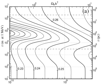
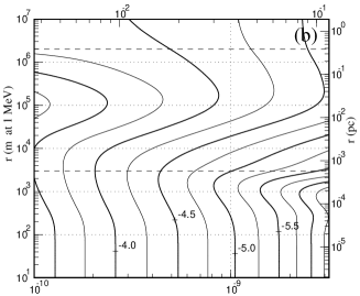
Figure 1.: The ⁴He, D, and ⁷Li yields from small-scale inhomogeneous nucleosynthesis runs with a centrally condensed geometry, with density contrast $R=800$ and high-density volume fraction $f_{v}=0.125$. The contours of (a) $Y_{p}$, (b) $\log_{10}$D/H, and (c) $\log_{10}{}^{7}$Li are plotted as a function of the average baryon-to-photon ratio $\eta$ and the distance scale $r$ of the inhomogeneity. The two horizontal dashed lines denote the horizon scale $\ell_{H}$ at the QCD (upper) and EW (lower) phase transitions. From Kainulainen et al. (1999).

2.2. Regions of Antimatter

A less-studied variant of IBBN is one where $\eta$ is allowed to have negative values, i.e., there are antimatter regions. This is possible in some baryogenesis scenarios (Dolgov 1996). Antimatter in cosmology has been reviewed by Steigman (1976). If the distance scale of antimatter regions is small, antimatter and matter will mix and annihilate in the early universe, and the presence of matter today implies that there was initially more matter than antimatter. If the distance scale is large, so that antimatter regions will survive till present, observational constraints require either the amount of antimatter to be very small, or the distance scale to be very large, comparable to the present horizon or larger (Cohen, De Rújula, & Glashow 1998), so that the case of large regions is not of interest for BBN.

The smaller the antimatter regions are, the earlier they annihilate. Rehm & Jedamzik (1998) considered annihilation immediately before nucleosynthesis. Kurki-Suonio & Sihvola (1999) extended these results to larger distance scales where annihilation occurs during or after nucleosynthesis (see Figure 2). So far the focus has been on obtaining upper limits to the amount of antimatter at various scales in the early universe, but clearly there is also potential for obtaining acceptable abundances with nonstandard values of $\eta$, although probably only with fine-tuned model parameters.

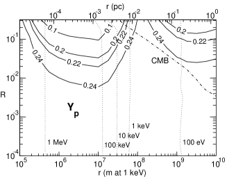
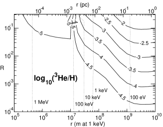
Figure 2.: The (a) ⁴He and (b) ³He yields as a function of the antimatter/matter ratio $R$ and the antimatter domain radius $r$. The distance scales are given both at $T=1$ keV (in meters) and today (in parsecs). We plot contours of $Y_{p}$ and (the logarithm of) the number ratio ³He/H. The dotted lines show contours of the “median annihilation temperature”, i.e., the temperature of the universe when 50% of the antimatter has annihilated. Typically the annihilation is complete at a temperature lower than this by about a factor of 3. The dot-dashed line gives the upper limit to $R$ from CMB spectrum distortion. This plot is for $\eta_{10}=6$. From Kurki-Suonio & Sihvola (1999).

3. Neutrinos and Big Bang Nucleosynthesis

Neutrinos affect BBN in two ways, through the energy density effect and the $\nu_{e}$ effect. The most significant effect is on $Y_{p}$ in both cases.

The energy density in neutrinos affects the expansion rate of the universe. The simplest way to increase the energy density of the early universe from the standard model is to have additional particle species (sterile neutrinos or other hypothetical particles). The custom is to parametrize this by an “effective number of neutrino species”. The standard case is $N_{\nu}=3$. We now know that there are only three “active” neutrino species, so any additional species must be “sterile” neutrinos or other very weakly interacting particles. A higher energy density means faster expansion. This leads to $n/p$ freezeout at a higher temperature, leaving more neutrons, and resulting in a higher ⁴He yield. The D yield is also increased, so an increased energy density is disfavored by BBN, and one gets an upper limit, e.g., $N_{\nu}<3.2$ (Burles et al. 1999) or $N_{\nu}\mathrel{\hbox{\hbox to0.0pt{\hbox{\lower 4.0pt\hbox{$\sim$}}\hss}\hbox{$<$}}}4$ (Lisi, Sarkar, & Villante 1999), depending on what observational constraints one uses.

Electron neutrinos affect the weak $n\leftrightarrow p$ reactions directly. More $\nu_{e}$ leads to fewer neutrons and thus to less ⁴He (and everything else), whereas more $\bar{\nu}_{e}$ leads to more neutrons and more ⁴He.

3.1. Neutrino Degeneracy

In SBBN one assumes that the neutrino asymmetry (difference between the number of neutrinos and antineutrinos),

$$L_{\nu}\equiv\frac{n_{\nu}-n_{\bar{\nu}}}{n_{\gamma}}=0.069\biggl{(}\frac{T_{\nu}}{T}\biggr{)}^{3}\bigl{(}\pi^{2}\xi+\xi^{3}),$$ (2)

which is related to the neutrino chemical potential $\mu_{\nu}$, or the degeneracy parameter $\xi\equiv\mu_{\nu}/T$, is small, $\ll 1$. This seems natural, since the comparable baryon asymmetry $\eta$ is small. However, the neutrino background is unobservable, so we cannot rule out a large neutrino asymmetry. A larger asymmetry always means a larger neutrino energy density, raising $N_{\nu}$. To have a significant effect on BBN, we must have $|\xi|$, $|L_{\nu}|\mathrel{\hbox{\hbox to0.0pt{\hbox{\lower 4.0pt\hbox{$\sim$}}\hss}\hbox{$>$}}}0.1$. There is a separate contribution from each neutrino flavor. Thus there are three indepedent degeneracy parameters, $\xi_{e}$, $\xi_{\mu}$, and $\xi_{\tau}$. The energy density effect is the same for all three flavors, and depends only on $|\xi|$. The electron neutrino effect depends only on $\xi_{e}$, but is much stronger, and the direction of the effect depends on the sign.

There are two possible scenarios for affecting BBN. If $\xi_{e}$ is comparable in magnitude to $\xi_{\mu}$ and $\xi_{\tau}$, or larger, one can forget the other two in first approximation. One can then adjust $\xi_{e}$ to dial in the desired value of $Y_{p}$. The other elements are hardly affected. A less natural scenario is one where the asymmetries in the other two neutrino flavors are much larger, and the energy density and $\nu_{e}$ effects are balanced against each other to keep $Y_{p}$ in the acceptable range. This way one can have a significant effect on the other abundances and raise the acceptable range for $\eta$. This second scenario is constrained by structure formation, since the large neutrino energy density means that the matter/radiation equality and thus the beginning of structure formation occurs later. Kang & Steigman (1992) used a generous lower limit for matter/radiation equality, $z_{\rm eq}>10^{3}$ to widen the SBBN acceptable range from $\eta_{10}$ = 2.8–4.7 to $\eta_{10}$ = 2.8–19.

3.2. Inhomogeneous Neutrino Degeneracy

The different results from high-$z$ D/H measurements (Tytler, Fan, & Burles 1996; Webb et al. 1997) raised the question whether there might be a large-scale inhomogeneity in primordial abundances. This is very difficult to achieve, since the extreme isotropy of the CMB rules out any significant large-scale inhomogeneity in $\eta$ or the energy density. Dolgov & Pagel (1999) have come up with a way of getting around this constraint. In their model the asymmetries of the different neutrino flavors are inhomogeneous but balanced with each other so that they add up to a homogeneous total energy density. The inhomogeneous $\xi_{e}$ is then responsible for the inhomogeneous primordial abundances through the $\nu_{e}$ effect. They suggest that an Afflect-Dine type scenario of generation of leptonic charge asymmetry, respecting the symmetry between different lepton families, could be responsible for creating a domain structure, where the neutrino asymmetries would have the same three values but interchanged with respect to $e$, $\mu$ and $\tau$. To achieve a significant D/H inhomogeneity, a huge $Y_{p}$ inhomogeneity has to be allowed. But since there are no high-$z$ $Y_{p}$ determinations, this cannot be used to rule out their model. Table 2 shows an example of what kind of abundances we could have in such a domain structure. The first line would correspond to our local domain; from the other domains we would have only D/H observations.

Table 2.: Abundances of light elements for $\eta_{10}=5$ and nonzero values of all three chemical potentials. One example from Dolgov & Pagel (1999).

$\xi_{e}$	$\xi_{\mu}$	$\xi_{\tau}$	D/H	$Y_{p}$	7Li/H
0.1	$-1$	1	$3.8\times 10^{-5}$	0.23	$2.5\times 10^{-10}$
$-1$	0.1	1	$9.2\times 10^{-5}$	0.55	$4.5\times 10^{-10}$
1	$-1$	0.1	$2.8\times 10^{-5}$	0.08	$1.1\times 10^{-10}$

3.3. Decay of a Massive Tau Neutrino

If the rest mass of a neutrino species is much larger than 100 MeV, then it is becoming nonrelativistic before nucleosynthesis and its contribution to the energy density is different from the standard zero-mass case. The laboratory limits for the neutrino masses leave this as a possibility for $\nu_{\tau}$. Above the neutrino decoupling temperature, $T\sim 3$ MeV, a massive neutrino species contributes less energy density, because of neutrino-antineutrino annihilation, but after neutrino decoupling the annihilation ceases and the rest mass then contributes extra energy density. Neutrinos this heavy must decay to avoid contributing too much to the present energy density. The decay time and mode are of crucial importance to BBN. If the decay time is very short, then the contribution to $N_{\nu}$ will be less than one. The most interesting case is the one where $\nu_{\tau}$ decays into $\nu_{e}$ (and a scalar particle), since then the $\nu_{e}$ effect could cause a significant reduction in $Y_{p}$.

These calculations are difficult since the decisive effects occur near the neutrino decoupling temperature, so thermal equilibrium is not maintained and the neutrino spectra are distorted. The recent results by Hannestad (1998) and Dolgov et al. (1999) are in disagreement with each other. Hannestad gets the maximum reduction of $Y_{p}$, from the SBBN result $Y_{p}=0.239$ to $Y_{p}<0.20$, for $\nu_{\tau}$ mass $m_{\nu}$ = 0.2–0.5 MeV and lifetime $\tau<100$ s. According to Dolgov et al., the maximum reduction is less, to $Y_{p}\sim 0.21$, and occurs for larger masses, $m_{\nu}$ = 2–3 MeV, and requires a shorter lifetime $\tau<1$ s.

The most natural explanation of the SuperKamiokande (1998) result on atmospheric neutrinos is $\nu_{\mu}\rightarrow\nu_{\tau}$ oscillation. Then $\nu_{\tau}$ cannot be heavy and its mass will not affect BBN significantly. To allow the above scenario, the atmospheric neutrino oscillations would have to be into a sterile neutrino species, $\nu_{\mu}\rightarrow\nu_{s}$, instead (Kainulainen et al. 1999).

3.4. Neutrino Oscillations

Observations of solar neutrinos and atmospheric neutrinos (SuperKamiokande 1998) as well as the LSND (1998) accelerator experiment see different amounts of the different neutrino flavors than predicted by the Standard Model. This can be explained by neutrino oscillations. This is a quantum-mechanical phenomenon where the flavor $(\nu_{e},\nu_{\mu},\nu_{\tau})$ content of the neutrino varies periodically. This requires nonzero neutrino masses and the effect is determined by the difference in mass-squared, $\Delta m^{2}$, and the “mixing angle”.

All three (solar, atmospheric, and LSND) “neutrino problems” cannot be simultaneously explained by oscillations among three flavors, but require at least a fourth flavor, $\nu_{s}$, which must be “sterile”, i.e., much more weakly interacting than the three known “active” flavors, in order not to violate the limit $N_{\nu}\sim 3$ from $Z^{0}$ decay width (Particle Data Group 1998). A sterile neutrino would also be useful for supernova nucleosynthesis (Peltoniemi 1996; Caldwell, Fuller, & Qian 1999).

The LSND results are controversial, so the other viewpoint is to ignore them until they are confirmed by independent experiments, in which case the solar and atmospheric neutrino problems can be explained just with the three active neutrinos.

Oscillations among (light, non-degenerate, i.e., $\xi=0$) active neutrinos do not affect BBN, since they all have equal abundances. If the sterile neutrino exists, it would have thermally decoupled from the other neutrinos very early, much before BBN, so that its contribution to $N_{\nu}$ would be $\ll 1$. Active-sterile neutrino oscillations before BBN would then lead to production of $\nu_{s}$, increasing $N_{\nu}$ (Enqvist, Kainulainen, & Thomson 1992), which from the BBN point of view is undesirable. The situation is more complicated, however. The oscillation depends on the background temperature, and at a certain temperature there is a resonance. This resonance temperature depends on the neutrino energy, so as the temperature falls, the resonance sweeps through the neutrino spectrum. If there is a small pre-existing asymmetry (this will be the case, since thermal fluctuations suffice), the rates of neutrino and antineutrino oscillation will be different. Resonant active–sterile neutrino oscillations will then lead to a growth of the neutrino asymmetry by a large factor (Barbieri & Dolgov 1991; Foot & Volkas 1995; Shi 1996; Enqvist, Kainulainen, & Sorri 1999; Di Bari & Foot 2000). This may generate a large enough electron neutrino asymmetry to affect BBN (Bell, Foot, & Volkas 1998; Kirilova & Chizhov 1998; Shi, Fuller, & Abazajian 1999).

Depending on the oscillation parameters, the asymmetry may either just grow or oscillate between positive and negative values, so that the final sign of the asymmetry becomes unpredictable. To calculate the effect on BBN is complicated, since the resulting distortion of the $\nu_{e}$ spectrum is also important for BBN, and the process happens near the neutrino decoupling temperature. There are two schemes to generate a large $\nu_{e}$ asymmetry, either directly via $\nu_{e}\leftrightarrow\nu_{s}$ oscillations or indirectly via $\nu_{\mu(\tau)}\leftrightarrow\nu_{s}$ and $\nu_{\mu(\tau)}\leftrightarrow\nu_{e}$ oscillations.

This scenario is under active study and there is much controversy among the different research groups. In Fig. 3 we show results obtained by Shi et al. (1999). The maximal effect on $Y_{p}$ seems to be at the $\pm 0.01$ level.

Figure 3.: The impact on the primordial ⁴He abundance $Y$ if an asymmetry in $\nu_{e}\bar{\nu}_{e}$ is generated by a resonant $\nu_{e}\leftrightarrow\nu_{s}$ mixing (left) or by the indirect neutrino mixing scheme (right), as a function of $\Delta m^{2}$. The baryon-to-photon ratio is set to $\eta=5.1\times 10^{-10}$. From Shi et al. (1999).

4. Conclusions

At present, no NSBBN scenario appears as convincing as SBBN, which is the simplest of all. Often the real world has turned out to be more complicated in the end than first assumed, but for the early universe a simple picture has been very successful. However, it is healthy to keep in mind the possibility that SBBN might not be the full story, and that any discrepancies between observations and SBBN might actually be telling us something important about the early universe or particle physics.

Acknowledgments.

I thank K. Kainulainen, A. Kalliomäki, J. Peltoniemi, and A. Sorri for advice on neutrino physics.

References

Applegate, J. H., Hogan, C. J., & Scherrer, R. J. 1987, Phys.Rev.D 35, 1151

Barbieri, R. & Dolgov, A. 1991, Nucl.Phys.B 237, 742

Bell, N. F., Foot, R., & Volkas, R. R. 1998, Phys.Rev.D 58, 105010

Burbidge, G., & Hoyle, F. 1998, ApJ 509, L1

Burles, S., Nollett, K. M., Truran, J. W., & Turner, M. S. 1999, Phys.Rev.Lett 82, 4176

Caldwell, D. O., Fuller, G. M., & Qian, Y.-Z. 1999, astro-ph/9910175

Cohen, A. G., De Rújula, A., & Glashow, S. L. 1998, ApJ 495, 539

Di Bari, P. & Foot, R. 2000, Phys.Rev.D, to be published, hep-ph/9912215

Dimopoulos, S., Esmailzadeh, R., Hall, L. J., & Starkman, G. D. 1988, ApJ 330, 545

Dolgov, A. D. 1996, in Proceedings of the International Workshop on Baryon Instability, Oak Ridge, March 1996, hep-ph/9605280

Dolgov, A. D., Hansen, S. H., Pastor, S., & Semikoz, D. V. 1999, Nucl.Phys.B 548, 385

Dolgov, A. D., & Pagel, B. E. J. 1999, New Astron 4, 223

Enqvist, K., Kainulainen, K., & Thomson, M. 1992, Nucl.Phys.B 373, 498

Enqvist, K., Kainulainen, K., & Sorri. A. 1999, Phys.Lett.B 464, 199

Foot, R. & Volkas, R. R. 1995, Phys.Rev.Lett 75, 4350

Hannestad, S. 1998, Phys.Rev.D 57, 2213

Hata, N., Scherrer, R. J., Steigman, G., Thomas, D., Walker, T. P., Bludman, S., & Langacker, P. 1995, Phys.Rev.Lett 75, 3977

Kainulainen, K., Kurki-Suonio, H., & Sihvola, E. 1999, Phys.Rev.D 59, 083505

Kang, H.-S., & Steigman, G. 1992, Nucl.Phys.B 372, 494

Kirilova, D. P. & Chizhov, M. V. 1998, Phys.Rev.D 58, 073004

Kurki-Suonio, H., & Sihvola, E. 1999, astro-ph/9912473

Leonard, R. E., & Scherrer, R. J. 1996, ApJ 463, 420

Lisi, E., Sarkar, S., & Villante, F. L 1999, Phys.Rev.D 59, 123520

LSND Collaboration (Athanassopoulos, C., et al.) 1998, Phys.Rev.Lett 81, 1774; Phys.Rev.C 58, 2489

Malaney, R. A., & Mathews, G. J. 1993, Phys.Rep 229, 145

Particle Data Group (Caso, C., et al.) 1998, Eur.J.Phys.C 3, 1

Peltoniemi, J. 1996, in Proceedings of the 3rd Tallinn Symposium on Neutrino Physics, ed. I. Ots, J. Lõhmus, P. Helde & L. Palgi, hep-ph/9511323

Rehm, J. B., & Jedamzik, K. 1998, Phys.Rev.Lett 81, 3307

Sarkar, S. 1996, Rep.Prog.Phys 59, 1493

Shi, X. 1996, Phys.Rev.D 54, 2753

Shi, X., Fuller, G. M., & Abazajian, K. 1999, Phys.Rev.D 60, 063002

Steigman, G. 1976, ARA&A 14, 339

Super-Kamiokande Collaboration (Fukuda, Y., et al.) 1998, Phys.Rev.Lett 81, 1562

Tytler, D., Fan, X. M., & Burles, S. 1996, Nature 381, 207

Webb, J. K., Carswell, R. F., Lanzetta, K. M., Ferlet, R., Lemoine, M., Vidal-Madjar, A., & Bowen, D. V. 1997, Nature 388, 250