Abstract

We present an overview of observational progress in the study of extragalactic globular cluster systems. Globular clusters turn out to be excellent tracers not only for the star-formation histories in galaxies, but also for kinematics at large galactocentric radii. Their properties can be used to efficiently constrain galaxy formation and evolution. After a brief introduction of the current methods and futures perspectives, we summarize the knowledge gained in various areas of galaxy research through the study of globular clusters. In particular, we address the star-formation histories of early-type galaxies; globular cluster population in late-type galaxies and their link to early-type galaxies; star and cluster formation during mergers and violent interactions; and the kinematics at large radii in early-type galaxies. The different points are reviewed within the context of galaxy formation and evolution.

Finally, we revisit the globular cluster luminosity function as a distance indicator. Despite its low popularity in the literature, we demonstrate that it ranks among one of the most precise distance indicators to early-type galaxies, provided that it is applied properly.

1 Preamble

This brief review on extragalactic globular cluster systems is derived from a lecture given for the award of the Ludwig-Bierman-Preis of the Astronomische Gesellschaft in Göttingen during September 1999. The Oral version aimed at introducing, mostly from an observer’s point of view, this field of research and at emphasizing its tight links to galaxy formation and evolution.

The scope of this written follow-up is not to give a complete review on globular cluster systems but to present recent discoveries, including examples, and to set them into the context of galaxy formation and evolution. The choice of examples and the emphasis of certain ideas will necessarily be subjective, and we apologize at this point for any missing references.

Excellent recent reviews can be found in the form of two books: “Globular Cluster Systems” by Ashman & Zepf (1998), as well as “Globular Cluster Systems” by Harris (2000). These include a full description of the globular clusters in the Local group (not discussed here), as well as an extensive list of references, including to older reviews.

The plan of the article is the following. In section 2, we give an introduction and the motivation for studying globular cluster systems with the aim of understanding galaxies. Section 3 presents current and future methods of observations, and the rational behind them. This section reviews recent progress in optical and near-infrared photometry and multi-object, low-resolution spectroscopy. It can be skipped by readers interested in results rather than methods. In Section 4 we present in turn the status of our knowledge on globular cluster systems in ellipticals, spirals and mergers. What are the properties of the systems? How are the galaxy types linked? And do mergers produce real ‘globular’ clusters? In section 5, we discuss sub-populations of globular clusters and their possible origin. The most popular scenarios to explain the presence of globular cluster sub-populations around galaxies are listed. The pros and cons, as well as the expectations of each scenario are discussed. We present, in section 6, some results from the study of globular cluster system kinematics. Finally, in section 7, we revisit the globular cluster luminosity function as a distance indicator. Under which conditions can it be used, and how should it be applied to minimize any systematic errors? It is compared to other distance indicators and shown to do very well. Some conclusions and an outlook are given in section 8.

2 Motivation

As a reminder, globular clusters are tyically composed of $10^{4}$ to $10^{6}$ stars clustered within a few parsecs. They are old, although young globular-cluster-like objects are seen in mergers, and their metallicity can vary between [Fe/H]$\simeq-2.5$ dex and [Fe/H]$>0.5$ dex. We refer to a globular cluster system as the totallity of globular clusters surrounding a galaxy.

2.1 Why study globular cluster systems?

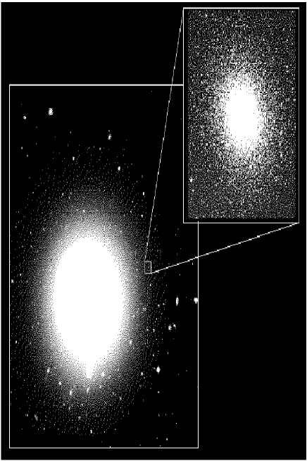
Figure 1: The figures shows a montage of what we are observing. The galaxy NGC 1399 of the Fornax galaxy cluster is shown on the left. It is located at a distance of $\sim 18$ Mpc from the Milky Way. Many of the point source surrounding it are globular clusters. If we could resolve these clusters into stars (which we cannot), we would see clusters similar to the Galactic clusters M 15, shown on the right.

The two fundamental questions in galaxy formation and evolution are: 1) When and how did the galaxies assemble? and 2) When and how did the galaxies form their stars? A third question could be whether, and to what extend, the two first points are linked.

Generally speaking, in order to answer these questions from an observational point of view, one can follow two paths. The first would be to observe the galaxies at high redshift, right at the epoch of their assembly and/or star formation. We will consider this to be the “hard way”. These observations are extremely challenging for many reasons (shifted restframe wavelength, faint magnitudes, small angular scales, etc…). Nevertheless, they are pursued by a number of groups through the observations of absorption line systems along the line of sights of quasars, or the detection of high-redshift (e.g. Lyman break) galaxies, etc… (see e.g. Combes, Mamon, & Charmandaris 1999, Bunker & van Breugel 1999, Mazure, Le Fevre, & Le Brun 1999 for recent proceedings on the rapidly evolving subject).

The second path is to wait until a galaxy reaches very low redshift and try to extract information about its past. This would be the “lazy way”. This is partly done by the study of the diffuse stellar populations at 0 redshift and the comparison of its properties at low redshift. Such studies on fundamental relations (fundamental plane, Mg-$\sigma$, Dn-$\sigma$) tend to be consistent with the stellar populations evolving purely passively and having formed at high redshifts ($z>2$). Alternatively, one can study merging events among galaxies at low- to intermediate-redshift (e.g. van Dokkum et al. 1999) in order to understand the assembly of galaxies.

How do globular clusters fit into these picture? Globular cluster studies could be classified as the “very lazy way”, since they reach out to at most redshifts of $z=0.03$. However, globular clusters are among the oldest objects in the universe, i.e. they witnessed most, if not all, of the history of their host galaxy. The goal of the globular cluster system studies is therefore to extract the memory of the system. Photometry and spectroscopy are used to derive their ages and chemical abundances which are used to understand the epoch(s) of star formation in the galaxy. Kinematic information obtained from the globular clusters (especially at large galactocentric radii) can be used to help understanding the assembly mechanism of the galaxies.

2.2 Advantages of using globular clusters

Figure 1 illustrates extragalactic globular cluster studies. We show the galaxy NGC 1399 surrounded by a number of point sources. If these point sources could be resolved, they would look like one of the Galactic globular clusters (here shown as M 15). However, even with diffraction limited imaging from space, we cannot resolve clusters at distances of 10 to 100 Mpc into single stars, and have to study their integrated properties. The study of a globular cluster system is therefore equivalent to studying the integrated properties of a large number of globular clusters surrounding a galaxy, in order to derive their individual properties and compare them, as well as the properties of the system as a whole, with the properties of the host galaxy.

The purely practical advantages of observing objects at $z=0$ is the possibility to study the objects in great detail. Very low $z$ observations are justified if the gain in details outbalances the fact that at high $z$ one is seeing events closer to the time at which they actually happened. One example that demonstrates that the gain is significant in the case of extragalactic globular clusters, is the discovery of several sub-populations of clusters around a large number of early-type galaxies. The presence of two or more distinct star-formation epochs/mechanisms in at least a large number if not all giant galaxies was not discovered by any other type of observations.

The old age of globular clusters is often advanced as argument for their study, since they witnessed the entire past of the galaxy including the earliest epochs. If this would be the whole truth, globular clusters would not be suited to study the recent star formation epochs. Nor would they present a real advantage over stars, which can be old too. What are the advantages of observing globular clusters as tracers of the star-formation / stellar populations instead of studying directly the diffuse stellar population of the host galaxies?

Globular clusters trace star formation

A number of arguments support the fact that globular clusters indeed trace the star formation in galaxies. However, we know that some star formation can occur without forming globular clusters. One example is the Large Magellanic Cloud which, at some epochs, produced stars but no clusters (e.g. Geha et al. 1998). On the other hand, we know that major star formation episodes induce the formation of a large number of star clusters. For example, the violent star formation in interacting galaxies is accompanied by the formation of massive young star clusters (e.g. Schweizer 1997). Also, the final number of globular clusters in a galaxy is roughly proportional to the galaxy luminosity, i.e. number of stars (see Harris 1991). This hints at a close link between star and cluster formation. Additional support for such a link comes from the close relation between the number of young star clusters in spirals and their current star formation rate (Larsen & Richtler 1999).

In summary, globular clusters are not perfect tracers for star formation, as they will not form during every single little (i.e. low rate) star formation event. But they will trace the major (violent) epochs of star formation, which is our goal.

From a practical point of view

Globular clusters exist around all luminous ($M_{V}>17$) galaxies observed to date. Their number, that scales with the mass of the galaxy, typically lies around a few hundreds to a few thousands.

Furthermore, globular clusters can be observed out to $\sim$ 100 Mpc. This is not as far as the diffuse light can be observed, but far enough to include many thousands of galaxies of all types and in all varieties of environments.

The study of globular clusters is therefore not restricted to a specific type or environment of galaxies: unbiased samples can be constructed. From this point of view, diffuse stellar light and globular clusters are equally appropriate.

The advantages of globular clusters over the diffuse stellar population

Globular clusters present a significant advantage when trying to determine the star formation history of a galaxy: they are far simpler structures. A globular cluster can be characterized by a single age and single metallicity, while the diffuse stellar population of a galaxy needs to be modeled by an unknown mix of ages and of metallicities. Studying a globular cluster system returns a large number of discrete age/metallicity data points. These can be grouped to determine the mean ages and chemical abundances of the main sub-populations present in the galaxy.

Along the same line, and as shown above, globular clusters form proportionally to the number of stars. That is, the number of globular clusters in a given population reflects the importance of the star formation episode at its origin. Counting globular cluster in different sub-populations indicates right away the relative importance of the different star formation events. In contrast, the different populations in the diffuse stellar light appear luminosity weighted: a small (in terms of mass) but recent star formation event can outshine a much more important but older event that has faded.

The bonus

As for stellar populations, kinematical informations can be derived from the spectra originally aimed at determining ages and metallicities. Globular clusters have the advantage that they can be traced out to galactocentric distances unreachable with the diffuse stellar light. The dynamical information of the clusters can be used to study the assembly of the host galaxy. In Section 6, we will come back to this point.

The bottom line is that globular clusters are good tracers for the star formation history of their host galaxies, and eventually allow some insight into their assembly too. They present a number of advantages over the study of stellar populations, and complement observations at high redshift. Their study allows new insight into galaxy formation and evolution.

3 Current and future observational methods

This section is intended to give a feeling for the observational methods used to study globular cluster systems. It addresses the problems still encountered in imaging and spectroscopy, as well as the improvements to be expected with future instruments.

To set the stage: we are trying to analyze the light of objects with typical half-light radii of 1 to 5 pc, at distances of 10 to 100 Mpc (i.e. half-light radii of 0.01${}^{{}^{\prime\prime}}$ to 0.1${}^{{}^{\prime\prime}}$ ), and absolute magnitudes ranging from $M_{V}\sim-10$ to $-4$ (i.e. $V>20$). The galaxies in the nearest galaxy clusters (Virgo, Fornax) have globular cluster luminosity functions that peak in magnitude around $V\sim 24$, and globular clusters have typical half-light radii of $\sim$ 0.05${}^{{}^{\prime\prime}}$ .

We intend to study both the properties of the individual clusters, as well as the ones of the whole cluster system. For the individual globular clusters, our goal is to derive their ages, chemical abundances, sizes and eventually masses. This requires spectral information (the crudest being just a color) and high angular resolution. For the whole system, our goal is to determine the total numbers, the globular cluster luminosity function, the spatial distributions (extent or density profile, ellipticity), and any radial dependencies of the cluster properties (e.g. metallicity gradients). These properties should also be measured for individual sub-populations, if they are present. The requirements for the systems are therefore deep, wide-field imaging, and the ability to distinguish potential sub-populations from each other.

3.1 Optical photometry

Globular clusters outside the Local Group were, for a long time, exclusively studied with optical photometry. Optical, ground-based photometry (reaching $V>24$ in a field $>$ 5${}^{{}^{\prime}}$$\times$ 5${}^{{}^{\prime}}$ ) turns out to be sufficient to determine most morphological properties of the systems (see Sect. 4). The depth allows to reasonably sample the luminosity function, and a field of several arcminutes a side usually covers the vast majority of the system.

Problems with optical photometry arise when trying to determine ages and metallicities. It is well known that broad-band optical colors are degenerate in age and metallicity (e.g. Worthey 1994). A younger age is compensated by a higher metallicity in most broad-band, optical colors. To some extent the problem is solved by the fact that most globular clusters are older than several Gyr, and colors do not depend significantly on age in that range. This, of course, means that deriving ages from optical colors is hopeless, except for young clusters as seen e.g. in mergers.

For old clusters, the goal is to find a color that is as sensitive to metallicity as possible. The widely used $V-I$ color is the least sensitive color to metallicity. $B-V$ and $B-I$ do better in the Johnson-Cousins system (e.g. Couture et al. 1991 for one of the first comparisons), but the mini break-through came with the use of Washington filters (e.g. Geisler & Forte 1990). These allowed the discovery of the first multi-modal globular cluster color distributions around galaxies (Zepf & Ashman 1993). However, the common use of the Johnson system, combined with large errors in the photometry at faint magnitudes, do still not allow a clean separation of individual globular clusters into sub-populations around most galaxies.

Another problem with ground-based imaging is that its resolution is by far insufficient to resolve globular clusters. This prohibits the unambiguous identification of globular clusters from foreground stars and background galaxies. In most cases the over-density of globular clusters around the host galaxy is sufficient to derive the general properties of the system. Control fields should be used (although often left out because of the lack of observing time), and statistical background subtraction performed. The individual identification of globular clusters became possible with WFPC2 on HST. Globular clusters appear barely extended in WFPC2 images, which allows on the one hand to reliably separate them from foreground stars and background galaxies, and on the other hand to systematically study for the first time globular cluster sizes outside the Local group (Kundu & Whitmore 1998, Puzia et al. 1999, Kundu et al. 1999). The disadvantage of WFPC2 observations is that the vast majority was carried out in $V-I$, the least performant system in terms of metallicity sensitivity. Furthermore, the WFPC2 has a small field of view which biases all the analysis towards the center of the galaxies, making it very hard to derive the global properties of a system without large extrapolations or multiple pointings.

In summary, ground-based photometry returns the general properties of the systems, and eventually of the sub-systems when high quality photometry is obtained. It suffers from confusion when identifying individual clusters, and is limited in age/metallicity determinations. Space photometry is currently as bad in deriving ages/metallicities, but allows to determine sizes of individual clusters. The current small fields, however, restrict the studies of whole systems.

Future progress is expected with the many wide-field imagers coming online, provided that deep enough photometry is obtained (errors $<0.05$ mag at $V=24$). These will provide a large number of targets for spectroscopic follow-up. In space, the ACS to be mounted on HST will superseed the WFPC2. The field of view remains modest, but the slightly higher resolution will support further size determinations, and the higher throughput will allow a more clever choice of filters, including $U$ and $B$.

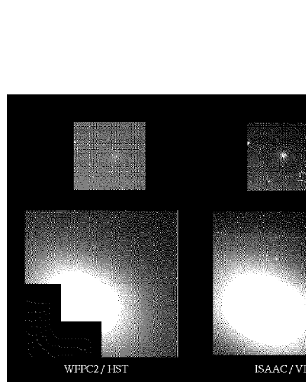
Figure 2: NGC 4365 observed in the V band with the WFPC2 on HST, and in the K band with ISAAC on the VLT. The field of views are similar; the resolution is $\sim 0.1"$ in the HST images, $\sim 0.4"$ in the K images; the depths are comparable. This illustrates that optical and near-infrared imaging are becoming more and more similar for purposes of studying globular cluster systems (images provided by T.H. Puzia).

3.2 Near-infrared photometry

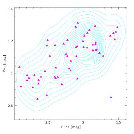
Figure 3: Globular cluster colors shown in the (V$-$I)–(V$-$K) plane. For this plot, data for NGC 3115 from ISAAC on the VLT and WFPC2 onboard HST were combined to allow a better separation of the two sub-populations (taken from Puzia et al. 2000, in preparation). Density contours show the color peaks for two main sub-populations.

Since the introduction of 1024$\times$1024 pixel arrays in the near infrared a couple of years ago, imaging at wavelength from 1.2$\mu$m to 2.5$\mu$m became competitive in terms of depths and field size with optical imaging (see Figure 2).

Historically, the first near-infrared measurements of extragalactic globular clusters were carried out in M31 (Frogel, Persson & Cohen 1980) and the Large Magellanic Cloud (Persson et al. 1983). Why extend the wavelength range to the near infrared? For old globular clusters, $V-K$ is a measure of the temperature of the red giant branch that is directly dependent on metallicity but hardly on age. $V-K$ is even more sensitive to metallicity than the Washington $C-T_{1}$ index. The combination of optical and near-infrared colors is therefore superior to optical imaging alone, both for deriving metallicities, and for a clean separation of cluster sub-populations (see Figure 3). It is also used to detect potential sub-populations were optical colors failed to reveal any.

In young populations, $V-K$ is most sensitive to the asymptotic giant branch which dominates the light of populations that are 0.2 to 1 Gyr old. The combination of optical and near infrared colors can be used to derive ages (and metallicities) of these populations (e.g. Maraston, Kissler-Patig, & Brodie 2000).

The disadvantages of complementing optical with near-infrared colors is the need for a second instrument (usually a second observing run) in addition to the optical one. Near-infrared observations will continue fighting against the high sky background in addition to the background light of the galaxy which requires blank sky observations. Overall, obtaining near-infrared data is still very time consuming when compared to optical studies. For example, a deep $K$ image of a galaxy will require a full night of observations. Currently both depth and field size do not allow the near infrared to fully replace optical colors for the study of morphological properties or the globular cluster luminosity function. But this might happen in the future whth the NGST.

The immediate future looks bright, with a number of “wide-field” imagers being available, such as ISAAC on the VLT, SOFI on the 3.5m NTT, the Omega systems on the 3.5m Calar Alto, etc.. and 2k $\times$ 2k infrared arrays coming soon. The ideal future instrument would have a dichroic which would allow to observe simultaneously in the near-infrared and the optical.

Figure 4: Three representative spectra of globular clusters are shown, ranging from blue, over red, to very red color. While the H$\beta$ gets slightly weaker from the blue to the red object, the metal lines (Mg, Fe, Na) become much stronger (taken from Kissler-Patig et al. 1998a).

3.3 Multi-object spectroscopy

Spectroscopy is the only way to unambiguously associate a globular cluster with its host galaxy by matching their radial velocities. Also, it is the most precise way to determine the metallicity of single objects, and the only way to determine individual ages. Obviously, it is also the only way to get radial velocities. Ideally, one would like a spectrum of each globular cluster identified from imaging.

In practice, good spectra are still hard to obtain. Early attempts with 4m-class telescopes succeeded in obtaining radial velocities, but mostly failed to determine reliable chemical abundances (see Sect. 6). With the arrival of 10m-class telescopes, it became feasible to obtain spectra with high enough signal-to-noise to derive chemical abundances (Kissler-Patig et al. 1998a, Cohen, Blakeslee & Ryzhov 1998). Such studies are still limited to relatively bright objects ($V<23$) and remain time consuming ($\sim$ 3h integration time for low-resolution spectroscopy). Figure 4 shows a few examples of globular clusters in NGC 1399. High-resolution spectroscopy in order to measure internal velocity dispersions of individual clusters is still out of reach for old clusters, and was only carried out for two nearby super star clusters (Ho & Fillipenko 1996a,b), in addition to several clusters within the Local Group. Even low-resolution spectroscopy is currently still limited to follow-ups on photometric studies, targeting a number of selected, representative clusters, rather than building up own spectroscopic samples.

Current problems are the low signal-to-noise, even with 10m-telescopes, that prohibit very accurate age or metallicity determinations for individual clusters. The multiplexity of the existing instruments (FORS1 & 2 on the VLT, LRIS on Keck) is low and only allows to spectroscopy a limited number of selected targets. Finally, the absorption indices that are being measured on the spectra in order to determine the various element abundances are not optimally defined. These indices lie in the region 3800Å to 6000Å and were designed for spectra with 8Å to 9Å resolution. They often include a number of absorption lines in the bandpass (or pseudo-continuum) other than the element to be measured. This introduces an additional dependence e.g. of the Balmer indices on metallicity, etc… Using a slightly higher resolution might help defining better indices.

The immediate future of spectroscopy are instruments such as VIMOS on the VLT or DEIMOS on Keck that will allow a multiplexity of 100 to 150. These will allow to increase the exposure times and slightly the spectral resolution to solve a number of the problems mentioned above. These will also allow to obtain several hundred radial velocities of globular clusters around a given galaxy in a single night, improving significantly the potential of kinematical studies (see Sect. 6).

4 Globular clusters in various galaxy types, and what we learned from them

In this section, we present some properties of globular cluster systems and of young clusters in ellipticals, spirals and mergers. In the last section we mentioned what are the properties measured in globular cluster systems: The metallicity distribution can be obtained from photometry (colors) or spectroscopy (absorption line indices). The luminosity function of the clusters is computed from the measured magnitudes folded with any incompleteness or contamination function. The total number of clusters (and eventually number of metal-poor and metal-rich clusters) is obtained by extrapolating the observed counts over the luminosity function and eventually applying any geometrical completeness for the regions that are not covered. For the latter, one uses also knowledge about the spatial distribution (position angle, ellipticity) and radial density profile of the globular cluster system. For young star clusters, the color distribution no longer reflects the metallicity distribution, but a mix of ages and metallicities. More complex comparisons with population synthesis models and/or spectroscopy are needed to disentangle the two quantities. Of interest for young clusters are also the mass distribution (derived from the luminosity function) that helps to understand how many of the newly formed clusters will indeed evolve into massive “globular” clusters.

4.1 Globular clusters in early-type galaxies

Early-type galaxies have the best studied globular cluster systems. Spirals have the two systems studied in most details (i.e. the Milky Way and M31) due to our biased location in space, but a far larger sample now exists for early-type galaxies.

Despite looking remarkably similar in many respects (e.g. globular cluster luminosity function), globular cluster systems in early-type galaxies also show a large scatter in a number of properties. For example, the number of globular clusters normalized to the galaxy light (specific frequency, see Harris & van den Bergh 1981) appears to scatter by a factor of several, mainly driven by the very high specific frequencies of central giant ellipticals (and recently also observed in faint dwarf galaxies, see Durrel et al. 1996, Miller et al. 1998). Furthermore, the radial density profiles are very extended for large galaxies, while following the galaxy light in the case of intermediate ellipticals (e.g. Kissler-Patig 1997a).

In the early 90’s, Zepf & Ashman (1993) discovered the presence of globular cluster sub-populations in several early-type galaxies. We will come back to the origin of the sub-populations in Sect. 5. Here, we will discuss the implications of sub-populations on our understanding of the globular cluster system properties.

Figure 5: Left panel: The angular distribution of halo and bulge globular clusters around NGC 1380 in 30 degree sectors, after a point symmetry around the center of the galaxy. Note that the blue objects are spherically distributed, while the red objects have an elliptical distribution that peaks at the position angle of the diffuse stellar light. Right panel: Surface density profiles of red and blue globular clusters around NGC 1380, plotted once against the radius in arcseconds (upper panel) and once against the semi-major axis (lower panel). Note how the blue objects have a much flatter density profile than the red ones, which are concentrated towards the center and follow a similar density profile as the stellar light. Both plots are taken from Kissler-Patig et al. (1997).

Until the early 90’s, properties were derived for the whole globular cluster system. Since then, it became clear that many properties need to take into account the existence of (at least two) different sub-populations, in order to be explained. Probably the first work to show this most clearly was the presentation of the properties of blue and red clusters in NGC 4472 by Geisler et al. (1996). Taking into account the existence and different spatial distribution of blue and red clusters, they explained two properties of whole systems at once. First, the color gradient observed in several systems could be explained by a varying ratio of blue to red clusters with radius (without any gradient in the individual sub-populations). Second, the mean color of the systems was previously thought to be systematically bluer than the diffuse galaxy light. It turns out that the color of the red sub-population matches the color of the galaxy, while it is the presence of the blue “halo” population that makes the color of the whole globular cluster system appear bluish.

It has not yet been demonstrated that the scatter in the specific frequency and in the slopes of the radial density profiles also originate from different mixes of blue to red sub-populations, but this could be the case. The few studies that investigated separately the morphological properties of blue and red clusters (Geisler et al. 1996, Kissler-Patig et al. 1997, Lee et al. 1998, Kundu & Whitmore 1998) found the metal-poor (blue) population to be more spherically distributed and extended than the metal-rich population that has a steeper density profile, tends to be more flattened and appears to follow the diffuse stellar light of the galaxy in ellipticity and position angle (cf. Fig. 5). Thus, a larger fraction of blue clusters in a galaxy would mimic a flatter density profile of the whole globular cluster system.

Furthermore, the specific frequency of the blue clusters (when related to the blue light) appears to be very high ($>30$ see Harris 2000). This, by the way, could be explained if the latter came from small fragments similar to the dwarf ellipticals observed today, that also show high specific frequency values (although not as high, but in the range 10 to 20). Thus, an overabundance of blue clusters would imply a high specific frequency. Incidentally, the shallow density profiles are found in the galaxies with the highest specific frequencies (see Kissler-Patig 1997a). We can therefore speculate that the properties of the entire globular cluster systems of these massive (often central) giant ellipticals can be explained by a large overabundance of metal-poor globular clusters originating from small fragments. The scatter in the globular cluster system properties among ellipticals could then (at least partly) be explained by a varying fraction of metal-poor “halo” and metal-rich “bulge” globular clusters.

Observationally, this could be verified by determining the number ratios of metal-rich and metal-poor globular clusters in a sample of galaxies showing different globular cluster radial density profiles and specific frequencies. The number of studies investigating the properties of metal-poor and metal-rich populations needs to increase in order to confirm the general properties of these two groups. We end with a word of caution: the existence of such sub-populations has been observed in only $\sim 50$% of all early-type galaxies studied (e.g. Gebhardt & Kissler-Patig 1999), and still remains to be demonstrated in all cases. Furthermore, the exact formation process of these sub-populations is still unclear (see Sect. 5).

4.2 Globular clusters in late-type galaxies

The study of globular cluster systems of late-type spirals started with the work of Shapley (1918) on the Milky Way system. Despite a head-start of nearly 40 years compared to studies in early-type galaxies, the number of studied systems in spirals lags far behind the one in ellipticals. This is mainly due to the observational difficulties: globular clusters in spirals are difficult to identify on the inhomogeneous background of disks. Furthermore, internal extinction in the spiral galaxies make detection and completeness estimations difficult, and photometry further suffers from confusion by reddened HII regions, open clusters or star forming regions.

The best studied cases (Milky Way and M31) show sub-populations (e.g. Morgan 1959, Kinman 1959, Zinn 1985; Ashman & Bird 1993, Barmby et al. 1999) associated in our Galaxy with the halo and the bulge/thick disk (Minniti 1995, Côté 1999). Beyond the local group, spectroscopy is needed to separate potential sub-populations. Both abundances and kinematics are needed, while colors suffer too much from reddening to serve as useful metallicity tracers. Spectroscopic studies have been rare in the past, but are now becoming feasible (see Sect. 3.3 and 4.1). For example, a recent study of M81 allowed to identify a potential thick disk population beside halo and bulge populations (see Schroder et al. 2000 and references therein).

Some of the open questions are whether all spirals host halo and bulge clusters, and whether one or both populations are related to the metal-poor and metal-rich populations in early-type galaxies. The number of globular clusters as traced by the specific frequency appears roughly constant in spirals of all types independently of the presence of a bulge and/or thick disk (e.g. Kissler-Patig et al. 1999a). This would mean that spirals are dominated by metal-poor populations, with their globular cluster systems only marginally affected by the presence of a bulge/thick disk. If metal-poor globular clusters indeed formed in pre-galactic fragments, then one would expect the metal-poor populations in spirals and ellipticals to be the same. We know that the globular cluster luminosity functions are extremely similar, but the metallicity distributions and other properties remain to be derived and compared (see Burgarella et al. 2000 for a first attempt). Finally, a good understanding of the globular cluster systems in spirals will also help predicting the resulting globular cluster system of a spiral–spiral merger. Predictions can then be compared to the properties of systems of elliptical galaxies in order to constrain this mode of galaxy formation.

4.3 Star clusters in mergers and violent interactions

After some speculations and predictions that massive star clusters could/should form in mergers (Harris 1981, Schweizer 1987), these were finally discovered in the early 90’s (Lutz 1991, Holtzman et al. 1992). Since then a number of studies focussed on the detection and properties of these massive young star clusters (see Schweizer 1997, and reviews cited in Sect. 1 for an overview).

The most intense debate around these young clusters focussed on whether or not their properties were compatible with a formation of early-type galaxies through spiral–spiral mergers. It was noticed early on (Harris 1981, van den Bergh 1982) that ellipticals appeared to host more clusters than spirals, and thus that mergers would have to produce a large number of globular clusters. Moreover, the specific frequency of ellipticals appeared higher than in spirals, i.e. mergers were supposed to form globular clusters extremely efficiently. In a second stage, a number of studies investigated whether or not these newly formed clusters would resemble globular clusters, and/or would survive as bound clusters at all.

The above questions are still open, except maybe for the last one. The young clusters studied to date show luminosities, sizes, and masses (when they can be measured) that are compatible with them being bound stellar clusters and able to survive the next several Gyr (see Schweizer 1997 for a summary of the studies and extensive references). Whether they will have the exact same properties as old globular clusters in our Milky Way is still controversial. First spectroscopic measurements found the young clusters in NGC 7252 compatible with a normal initial mass function (IMF) (Schweizer & Seitzer 1998), while in NGC 1275 the young clusters show anomalies and potentially have a flatter IMF (Brodie et al. 1998) which would compromise their evolution into old globular clusters, as we know them from the Galaxy.

The mass distribution of these young cluster was first found to be a power-law (e.g. Meurer 1995), as opposed to a log-normal distribution for old globular clusters. This result is likely to suffer from uncertainties in the conversion of luminosities into masses, when neglecting the significant age spread among the young clusters (see Fritze-von Alvensleben 1999). However, deeper data seem to rule out the possibility that the initial mass distribution has already the same shape as the one observed for old clusters (see Whitmore et al. 1999, Zepf et al. 1999). But the slope of the mass distributions could be affected during the evolution of the system by dynamical destruction at the low-mass end. Finally, Whitmore et al. (1999) recently found a break in the mass function of the young clusters of the Antennae galaxies, similar to the characteristic mass of the old clusters further supporting similar mass functions for young and old cluster populations (see also Sect. 7). Overall, the young clusters might or might not resemble old Galactic globular clusters, but some will survive as massive star clusters and could mimic a population of metal-rich globular clusters.

The most interesting point remains the number of clusters produced in mergers. Obviously, this will depend on the gas content (‘fuel’) that is provided by the merger (e.g. Kissler-Patig, et al. 1998b). Most gas-rich mergers form a large number of star clusters, but few of the latter have masses that would actually allow them to evolve into massive globular clusters as we observe them in distant ellipticals. Harris (2000) reviews comprehensively this issue and other problems related with a scenario in which all metal-rich globular clusters of ellipticals would have formed in mergers. The main problem with such a scenario is that the high specific frequency of ellipticals should be due to metal-rich clusters, which is usually not the case. Potential other problems, depending on the exact enrichment history, are that large ellipticals would be build up by a series of mergers that should probably produce an even broader metallicity distribution than observed; and that radial metallicity gradients might be expected to be steeper in high specific frequency ellipticals.

In summary, mergers are the best laboratories to study younger stellar populations and the formation of young stellar cluster, but how important they are in the building of globular cluster systems (and galaxies) remains uncertain. However, a good understanding of these clusters is crucial for the understanding of globular cluster systems in early-type galaxies, since merger events must have played a role at some stage.

5 Globular cluster sub-populations and their origin

In this section we come back to the presence of multiple sub-population of globular clusters around a number of giant galaxies. We will briefly review the different scenarios present in the literature that could explain the properties of such composite systems and discuss their pros and cons.

Sub-populations of globular clusters were first identified in the Milky Way (Morgan 1959, Kinman 1959, Zinn 1985), and associated with the halo (in the case of the metal-poor population) and the “disk” (in the case of the metal-rich population. The “disk” clusters are now better associated with the bulge (e.g. Minniti 1995, Côté 1999). The presence of multiple component populations in other giant galaxies was first detected by Zepf & Ashman (1993). Obviously the multiple sub-populations get associated with several distinct epochs or mechanisms of star/cluster formation.

The simple scenario of a disk–disk merger explaining the presence of two populations of globular clusters (Ashman & Zepf 1992) found a strong support in the community for 5-6 years, partly because of a lack of alternatives. It was backed up by the discovery of newly formed, young star clusters in interacting galaxies (Lutz et al. 1991, Holtzman et al. 1992). Only recently, other scenarios explaining the presence of at least two distinct populations were presented and discussed.

5.1 The different scenarios for sub-populations

We will make a (somewhat artificial) separation in four scenarios and briefly outline them and their predictions.

The merger scenario

The fact that mergers could produce new globular clusters was mentioned in the literature early after Toomre (1977) proposed that ellipticals could form out of the merging of two spirals (see Harris 1981 and Schweizer 1987). But the first crude predictions of the spiral-spiral merger scenario go back to Ashman & Zepf (1992). They predicted two populations of globular clusters in the resulting galaxy: one old, metal-poor population from the progenitor spirals and one newly formed, young, metal-rich population. The metal-poor population would be more extended and would have been transfered some of the orbital angular momentum by the merger. The metal-rich globular clusters would be more concentrated towards the center and probably on more radial orbits.

In situ scenarios

In situ scenarios see all globular clusters forming within the entity that will become the final galaxy. In this scenario, globular clusters form in the collapse of the galaxy, which happens in two distinct phases (see Forbes et al. 1997, Harris et al. 1998, Harris et al. 1999). The first burst produces metal-poor globular clusters and stars (similar to Searle & Zinn 1978) and provokes its own end e.g. by ionizing the gas or expelling it (e.g. Harris et al. 1998). The second collapse happens shortly later (1-2 Gyr) and is at the origin of the metal-rich component. Both populations are linked with the initial galaxy.

Accretion scenarios

Accretion scenarios were reconsidered in detail to explain the presence of the large populations of metal-poor globular clusters around early-type galaxies. In these scenarios, the metal-rich clusters belong to the seed galaxy, while the metal-poor clusters are accreted from or with dwarf galaxies (e.g. Richtler 1994). Côté et al. (1998) showed in extensive simulations that the color distributions could be reproduced. Hilker (1998) and Hilker et al. (1999) proposed the accretion of stellar as well as gas-rich dwarfs that would form new globular when accreted. In such scenarios, the metal-poor clusters would not be related to the final galaxies but rather have properties compatible with that of globular clusters in dwarf galaxies. Furthermore, this scenario is the only one that could easily explain metal-poor cluster that are younger than metal-rich ones. In a slightly differently scenario, Kissler-Patig et al. (1999b) mentioned the possibility that central giant ellipticals could have accreted both metal-poor and metal-rich clusters from surrounding medium-sized galaxies.

Pre-galactic scenarios

Pre-galactic scenarios were proposed long ago by Peebles & Dicke (1968), when the Jeans mass in the early universe was similar to globular cluster masses. Meanwhile, it was reconsidered in the frame of globular cluster systems (Kissler-Patig 1997b, Kissler-Patig et al. 1998b, Burgarella et al. 2000). The metal-poor globular clusters would have formed in fragments before the assembly of the galaxy, later-on building up the galaxy halos and feeding with gas the formation of the bulge. In that scenario too, the metal-poor globular clusters do not have properties dependent from the final galaxy, while the metal-rich clusters do. Also, metal-poor clusters are older than metal-rich clusters.

Overall, the scenarios are discussed in the literature as different but do not differ by much. The first scenario explains the presence of the metal-rich population, as opposed to the last two that deal with the metal-poor population. These three scenarios are mutually not exclusive. Only in situ models connect the metal-rich and metal-poor components. For the metal-rich clusters, the question resumes to whether they formed during the collapse of the bulge/spheroid, or whether they formed in a violent interaction. Although an early, gas-rich merger event at the origin of the bulge/spheroid would qualify for both scenarios. In the case of metal-poor clusters, the difference between the last three scenarios is mostly semantics. They differ slightly on when the clusters formed, and models two and four might expect differences in whether or not the properties of the clusters are related to the final galaxy. But the bottom line is that the boarder-line between the scenarios is not very clear. Explaining the building up of globular cluster systems is probably a matter of finding the right mix of the above mechanisms, and this for every given galaxy.

5.2 Pros and cons of the scenarios

The predictions of the different scenarios are fairly fuzzy, and no scenario makes clear, unique predictions. Nevertheless, we can present the pros and cons to outline potential problems with any of them.

The merger scenario

Pros: we know that new star cluster form in mergers (e.g. above mentioned reviews, and see Schweizer 1997), and will populate the metal-rich sub-population of the resulting galaxy. Note also, that the merger scenario is the only one that predicted bimodal color distributions rather then explaining them after fact.

Cons: we do not know i) if all early-type galaxies formed in mergers, ii) if the star clusters formed in mergers will indeed evolve into globular clusters (e.g. Brodie et al. 1998), iii) if all mergers produce a large number of clusters (which depends on the gas content). Furthermore, we would then expect the metal-rich populations to be significantly younger in many galaxies (according e.g. to the merger histories predicted by hierarchical clustering models). There are still problems in explaining the specific frequencies and the right mix of blue and red clusters in early-type galaxies in the frame of the merger scenario (e.g. Forbes et al. 1997).

In situ scenarios

Pros: Searle & Zinn (1978) list the evidences for our Milky Way halo globular clusters to have formed in fragments building up the halo. The massive stars in such a population would quickly create a hold of the star/cluster formation for a Gyr or two.

Cons: if a correlation between metal-poor clusters and galaxy is expected, the scenario would be ruled out. A clear age sequence from metal-poor to metal-rich clusters is predicted but not yet verified. This scenarios is not in line with hierarchical clustering models for the formation of galaxies (Kauffmann et al. 1993, Cole et al. 1994), should the latter turn out to be the right model for galaxy formation.

Accretion scenarios

Pros: dwarf galaxies are seen in great numbers around giant galaxies, and hierarchical clustering scenarios predict even more at early epochs. Dwarf galaxies do get accreted (e.g. Sagittarius in our Galaxy). We observe “free-floating” populations around central cluster galaxies (e.g. Hilker et al. 1999) and the color distributions of globular cluster systems can be reproduced (Côté et al. 1998).

Cons: we are missing detailed dynamical simulations of galaxy groups and clusters to test whether the predicted large number of dwarf galaxies gets indeed accreted (and when). We do not know whether the (dwarf) galaxy luminosity function was indeed as steep as required at early times to explain the large accretion rates needed. Also, the model does not provide a physical explanation for the metal-rich populations.

Pre-galactic scenarios

Pros: similar to the above, we observe a “free-floating”, spatially extended populations of globular clusters around central galaxies. The properties of the metal-poor populations do not seem to correlate with the properties of their host galaxies (Burgarella et al. 2000). The metal-poor globular cluster are observed to be very old (e.g. Ortolani et al. 1995 for our Galaxy; Kissler-Patig et al. 1998a, Cohen et al. 1998, Puzia et al. 1999 for analogies in extragalactic systems).

Cons: galaxies and galaxy halos might not have formed by the agglomeration of independent fragments. No physical model exists, except a broad compatibility with hierarchical clustering models (see also Burgarella et al. 2000).

Some pros and cons are listed only under one scenario but apply obviously to others. It should be noted that these pros and cons apply to “normal” globular cluster systems. It has been noted that several galaxies host very curious mixes of metal-poor and metal-rich clusters (Gebhardt & Kissler-Patig 1999, Harris et al. 2000) that pose challenges to all scenarios. Fine difference will require a much more detailed abundance analysis of the individual clusters in sub-populations, as well as their dynamical properties and (at least relative) ages for the different globular cluster populations. These might allow to identify a unique prediction supporting the one or the other formation mode, or constrain the importance of each formation mechanism.

6 Kinematics of globular clusters

Figure 6: Velocity dispersion as a function of radius for various components around NGC 1399, see Kissler-Patig et al. (1998a) for details. The two solid lines are fits to the velocity data of the globular clusters and of the Fornax galaxies. The dashed line shows the X–ray temperature converted to a velocity dispersion, the triangles are stellar measurements.

Figure 7: Kinematics of red (thin line) and blue (thick line) globular clusters in M87. Projected velocity dispersion, and projected rotational velocity as functions of radius for a fixed position angle of 120^∘. Dotted lines mark the 68% confidence bands. Taken from Kissler-Patig & Gebhardt 1998.

In this section, we briefly discuss recent results from kinematical studies of extragalactic globular clusters. The required measurements were discussed in Sect. 3. Kinematics can be used both to understand the formation of the globular cluster systems, as well as to derive dynamics of galaxies at large radii.

6.1 Globular cluster system formation

Globular cluster system kinematics are used since a long time to constrain their formation. In the Milky Way, kinematics support the association of the various clusters with the halo and the bulge (see Harris 2000 and references therein). In M31, similar results were derived (Huchra et al. 1991, Barmby et al. 1999). In M81, the situation appears very similar again (Schroder et al. 2000). Beyond the Local group, radial velocities for globular clusters are somewhat harder to obtain. Nevertheless, studies of globular cluster kinematics in elliptical galaxies started over a decade ago (Mould et al. 1987, 1990, Huchra & Brodie 1987, Harris 1988, Grillmair et al. 1994).

Figure 6 illustrates one example where the kinematics of globular clusters allowed to gain some insight into the globular cluster system formation (from Kissler-Patig et al. 1999b). The figure shows the velocity dispersion as a function of radius around NGC 1399, the central giant elliptical in Fornax. The velocity dispersion of the globular clusters increases with radius, rising from a value not unlike that for the outermost stellar measurements at 100${}^{{}^{\prime\prime}}$, to values almost twice as high at $\sim$ 300${}^{{}^{\prime\prime}}$. The outer velocity dispersion measurements are in good agreement with the temperature of the X-ray gas and the velocity dispersion of galaxies in the Fornax cluster. Thus, a large fraction of the globular clusters which we associate with NGC 1399 could rather be attributed to the whole of the Fornax cluster. By association, this would be true for the stars in the cD envelope too. This picture strongly favors the accretion or pre-galactic scenarios for the formation of the metal-poor clusters in this galaxy.

As another example, Fig. 7 shows the velocity dispersion and rotational velocity for the metal-poor and metal-rich globular clusters around M87, the central giant elliptical in Virgo. There is some evidence that the rotation is confined to the metal–poor globular clusters. If, as assumed, the last merger was mainly dissipationless (and did not form a significant amount of metal-rich clusters), this kinematic difference between the two sub–populations could reflect the situation in the progenitor galaxies of M87. These would then be compatible (see Hernquist & Bolte 1992) with a formation in a gas-rich merger event (see Ashman & Zepf 1992).

Generally, the data seem to support the view that the metal-poor globular clusters form a hot system with some rotation, or tangentially biased orbits. The metal-rich globular clusters have a lower velocity dispersion in comparison, and exhibit only weak rotation, if at all (Cohen & Ryzhov 1997, Kissler-Patig et al. 1999b, Sharples et al. 1999, Kissler-Patig & Gebhardt 1999, Cohen 2000). The interpretation of these results in the frame of the different formation scenarios presented in Sect. 5 is unclear, since no scenario makes clear and unique predictions for the kinematics of the clusters. Furthermore, some events unrelated to the formation of the globular clusters can alter the dynamics: e.g. a late dissipationless mergers of two ellipticals could convey angular momentum to both metal-rich and metal-poor clusters, bluring kinematical signatures present in the past. Detailed dynamical simulations of globular cluster accretion and galaxy mergers are necessary in order to compare the data with scenario predictions. But clearly, kinematics can help understanding differences in the metal-poor and metal-rich components, exploring intra-cluster globular clusters, and studying the formation of globular cluster systems as a whole.

6.2 Galaxy dynamics

Kinematical studies of globular clusters can also be used to study galaxy dynamics. The globular clusters do only represent discrete probes in the gravitational potential of the galaxy, as opposed to the diffuse stellar light that can be used as a continuous probe with radius, but globular clusters have the advantage (such as planetary nebulae) to extend further out. Globular clusters can be measured out to several effective radii, probing the dark halo and dynamics at large radii.

The velocity dispersion around NGC 1399, presented above, is one example. Another example was presented by Cohen & Ryzhov (1997) who derived from the velocity dispersion of the globular clusters in M87 a mass of $3\times 10^{12}M_{\odot}$ at 44kpc and a mass-to-light ratio $>30$, strongly supporting the presence of a massive dark halo around this galaxy. With the same data, Kissler-Patig & Gebhardt (1998) derived a spin for M87 of $\lambda\sim 0.2$, at the very high end of what is predicted by cosmological N-body simulations. The authors suggested as most likely explanation for the data a major (dissipationless) merger as the last major event in the building of M87.

These examples illustrate what can be learned about the galaxy formation history from kinematical studies of globular cluster system. In the future, instruments such as VIMOS and DEIMOS will allow to get many hundreds velocities in a single night for a given galaxy. These data will allow to constrain even more strongly galaxy dynamics at large radii.

7 Globular clusters as distance indicators

In this section, we will review the globular cluster luminosity function (GCLF) as a distance indicator. The method is currently “unfashionable” in the literature mainly because some previous results seem to be in contradiction with other distance indicators (e.g. Ferrarese et al. 1999). We will try to shade some light on the discrepancies, and show that, if the proper corrections are applied, the GCLF competes well with other extragalactic distance indicators.

7.1 The globular cluster luminosity function

A nice overview of the method is given in Harris (2000), including some historical remarks and a detailed description of the method. A further review on the GCLF method was written by Whitmore (1997), who addressed in particular the errors accompanying the method. We will only briefly summarize the method here.

The basics of the method are to measure in a given filter (most often $V$) the apparent magnitudes of a large number of globular clusters in the system. The so constructed magnitude distribution, or luminosity function, peaks at a characteristic (turn-over) magnitude. The absolute value for this characteristic magnitude is derived from local or secondary distance calibrators, allowing to derive a distance modulus from the observed turn-over magnitude. Figure 8 shows a typical globular cluster luminosity function with its clear peak (taken from Della Valle et al. 1998).

Figure 8: Typical GCLF, observed in the $V$ band in the galaxy NGC 1380 (Della Valle et al. 1998). Over-plotted are two fits (a Gaussian and a student t₅ function). The dotted lines show the 50% completeness limit in the $V$ filter and in the filter combination ($B,V,R$) that was used to select the globular clusters. The apparent peak magnitude can be derived and the distance computed using the absolute magnitude obtained from local or secondary calibrators.

The justification of the method is mainly empirical. Apparent turn-overs for galaxies at the same distance (e.g. in the same galaxy cluster) can be compared and a scatter around 0.15 mag is then obtained, without correcting for any external error. Similarly, a number of well observed apparent turn-over magnitudes can be transformed into absolute ones using distances from other distance indicators (Cepheids where possible, or a mean of Cepheids, surface brightness fluctuations, planetary luminosity function, …) and a similar small scatter is found (see Harris 2000 for a recent compilation). Taking into account the errors in the photometry, the fitting of the GCLF, the assumed distances, etc… this hints at an internal dispersion of the turn-over magnitude of $<0.1$, making it a good standard candle. From a theoretical point of view, this constancy of the turn-over magnitude translates into a “universal” characteristic mass in the globular cluster mass distributions in all galaxies. Whether this is a relict of a characteristic mass in the mass function of the molecular clouds at the origin of the globular clusters, or whether it was implemented during the formation process of the globular clusters is still unclear.

The absolute turn-over magnitude lies around $V_{TO}\sim-7.5$, and the determination of the visual turn-over is only accurate if the peak of the GCLF is reached by the observations. From an observational point of view, this means that the data must reach e.g. $V\sim 25$ to determine distances in the Fornax or Virgo galaxy clusters (D$\sim 20$ Mpc), and that with HST or 10m-class telescopes reaching typically $V\sim 28$, the method could be applied as far out as 120 Mpc (including the Coma galaxy cluster).

The observational advantages of this method over others are that globular clusters are brighter than other standard candles (except for supernovae), and do not vary, i.e. no repeated observations are necessary. Further, they are usually measured at large radii or in the halo of (mostly elliptical) galaxies where reddening is not a concern.

7.2 General problems

A large number of distance determinations from the GCLF were only by-products of globular cluster system studies, and often suffered from purely practical problems of data taken for different purposes.

First, a good estimation of the background contamination is necessary to clean the globular cluster luminosity function from the luminosity function of background galaxies which tends to mimic a fainter turn-over magnitude. Next, the finding incompleteness for the globular clusters needs to be determined, in particular as a function of radius since the photon noise is changing dramatically with galactocentric radius. Proper reddening corrections need to be applied and might differ whether one uses the “classical” reddening maps of Burstein & Heiles (1984) or the newer maps from Schlegel et al. (1998). When necessary, proper aperture correction for slightly extended clusters on WFPC2/HST images has to be made (e.g. Puzia et al. 1999). Finally, several different ways of fitting the GCLF are used: from fitting a histogram, over more sophisticated maximum-likelihood fits taking into account background contamination and incompleteness. The functions fitted vary from Gaussians to Student (t₅) functions, with or without their dispersion as a free parameter in addition to the peak value.

In addition to these, errors in the absolute calibration will be added (see below). Furthermore, dependences on galaxy type and environment were claimed, although the former is probably due to the mean metallicity of globular clusters differing in early- and late-type galaxies, while the latter was never demonstrated with a reliable set of data.

All the above details can introduce errors in the analysis that might sum up to several tenths of a magnitude. The fact that distance determinations using the GCLF are often a by-product of studies aiming at understanding globular cluster or galaxy formation and evolution, did not help in constructing a very homogeneous sample in the past. The result is a very inhomogeneous database (e.g. Ferrarese et al. 1999) dominated by large random scatter introduced in the analysis, as well as systematic errors introduced by the choice of calibration and the complex nature of globular cluster systems (see below). Nevertheless, most of these problems were recognized and are overcome by better methods and data in the recent GCLF distance determinations.

7.3 The classical way: using all globular clusters of a system

Harris (2000, see also Kavelaars et al. 2000) outline what we will call the classical way of measuring distances with the GCLF. This method implies that the GCLF is measured from all globular clusters in a system. In addition, it uses the GCLF as a “secondary” distance indicator, basing its calibration on distances derived by Cepheids an other distance indicators. The method compares the peak of the observed GCLF with the peak of a compilation of GCLFs from mostly Virgo and Fornax ellipticals, adopting from the literature a distance to these calibrators. This allowed, among others, Harris’ group to determine a distance to Coma ellipticals and to construct the first Hubble diagram from GCLFs in order to derive a value for H₀ (Harris 2000, Kavelaars et al. 2000).

In practice, an accurate GCLF turn-over is determined (see above) and calibrated without any further corrections using M${}_{V}(TO)=-7.33\pm 0.04$ (Harris 2000) or M${}_{V}(TO)=-7.26\pm 0.06$ using Virgo alone (Kavelaars et al. 2000).

The advantages of this approach are the following. Using all globular clusters (instead of a limited sub-population) often avoids problems with small number statistics. This is also the idea behind using Virgo GCLFs instead of the spars Milky Way GCLF as calibrators. The Virgo GCLFs, derived from giant elliptical galaxies rich in globular clusters, are well sampled and do not suffer from small number statistics. Further, since most newly derived GCLFs come from cluster ellipticals, one might be more confident to calibrate these using Virgo (i.e. cluster) ellipticals, in order to avoid any potential dependence on galaxy type and/or environment.

However, the method has a number of caveats. The main one is that giant ellipticals are known to have globular cluster sub-populations with different ages and metallicities. This automatically implies that the different sub-populations around a given galaxy will have different turn-over magnitudes. By using the whole globular cluster systems, one is using a mix of turn-over magnitudes. One could in principal try to correct e.g. for a mean metallicity (as proposed by Ashman, Conti & Zepf 1995), but this correction depends on the population synthesis model adopted (see Puzia et al. 1999) and implies that the mix of metal-poor to metal-rich globular clusters is known. This mix does not only vary from galaxy to galaxy (e.g. Gebhardt & Kissler-Patig 1999), but also varies with galactocentric radius (e.g. Geisler et al. 1996, Kissler-Patig et al. 1997). It results in a displacement of the turn-over peak and the broadening of the observed GCLF of the whole system. The Virgo ellipticals are therefore only valid calibrators for other giant ellipticals with a similar ratio of metal-poor to metal-rich globular clusters and for which the observations cover similar radii. This is potentially a problem when comparing ground-based (wide-field) studies with HST studies focusing on the inner regions of a galaxy. Or when comparing nearby galaxies where the center is well sampled to very distant galaxies for which mostly halo globulars are observed. In the worse case, ignoring the presence of different sub-populations and comparing very different galaxies in this respect, can introduce errors a several tenths of magnitudes.

Another caveat of the classical way, is that relative distances to Virgo can be derived, but absolute magnitudes (and e.g. values of H₀) will still dependent on other methods such as Cepheids, surface brightness fluctuations (SBF), Planetary Nebulae luminosity functions (PNLF), and tip of red-giant branches (TRGB), i.e. the method will never overcome these other methods in accuracy and carry along any of their potential systematic errors.

7.4 The alternative way: using metal-poor globular clusters only

As an alternative to the classical way, one can focus on the metal-poor clusters only. The idea is to isolate the metal-poor globular clusters of a system and to determine their GCLF. As a calibrator, one can use the GCLF of the metal-poor globular clusters in the Milky Way, which avoids any assumption on the distance of the LMC and will be independent of any other extragalactic distance indicator. For the Milky Way GCLF, the idea is to re-derive an absolute distance to each individual cluster, resulting in individual absolute magnitudes and allowing to derive an absolute luminosity function. Individual distances to the clusters are derived using the known apparent magnitudes of their horizontal branches and a relation between the absolute magnitude of the horizontal branch and the metallicity (e.g. Gratton et al. 1997). The latter is based on HIPPARCOS distances to sub-dwarfs fitted to the lower main sequence of chosen clusters. This methods follows a completely different path than methods based at some stage on Cepheids. In particular, the method is completely independently from the distance to the LMC.

In practice, an accurate GCLF turn-over (see above) for the metal-poor clusters in the target galaxy is derived and calibrated, without any further corrections, using M${}_{V}(TO)=-7.62\pm 0.06$ derived from the metal-poor clusters of the Milky Way (see Della Valle et al. 1998, Drenkhahn & Richtler 1999; note that the error is statistical only and does not include any potential systematic error associated with the distance to Galatic globular clusters, currently under debate).

The advantages of this method are the following. This method takes into account the known sub-structures of globular cluster systems. Using the metal-poor globular clusters is motivated by several facts. First, they appear to have a true universal origin (see Burgarella et al. 2000), and their properties seem to be relatively independent of galaxy type, environment, size and metallicity. Thus, to first order they can be used in all galaxies without applying any corrections. In addition, the Milky Way is justified as calibrator even for GCLFs derived from elliptical galaxies. Further, they appear to be “halo” objects, i.e. little affected by destruction processes that might have shaped the GCLF in the inner few kpc of large galaxies, or that affect objects on radial orbits. They will certainly form a much more homogeneous populations than the total globular cluster system (see previous sections). Using the Milky Way as calibrator allows this method to be completely independent on other distance indicators and to check independently derived distances and value of H₀.

The method is not free from disadvantages. First, selecting metal-poor globular clusters requires better data than are currently used in most GCLF studies, implying more complicated and time-consuming observations. Second, even with excellent data a perfect separation of metal-poor and metal-rich clusters will not be possible and the sample will be somewhat contaminated by metal-rich clusters. Worse, the sample size will be roughly halved (for a typical ratio of blue to red clusters around one). This might mean that in some galaxies less than hundred clusters will be available to construct the luminosity function, inducing error $>0.1$ on the peak determination due to sample size alone. Finally, the same concerns applies as for the whole sample: how universal is the GCLF peak of metal-poor globular clusters? This remains to be checked, but since variations of the order of $<0.1$ seem to be the rule for whole samples, there is no reason to expect a much larger scatter for metal-poor clusters alone.

7.5 A few examples, comparisons, and the value of H₀ from the GCLF method

Two examples of distance determinations from metal-poor clusters were given in Della Valle et al. (1998), and Puzia et al. (1999).

The first study derived a distance modulus for NGC 1380 in the Fornax cluster of $(m-M)=31.35\pm 0.09$ (not including a potential systematic error of up to 0.2). In this case, the GCLF of the metal-poor and the metal-rich clusters peaked at the same value, i.e. the higher metallicity was compensated by a younger age (few Gyr) of the red globular cluster population, so that it would not make a difference whether one uses the metal-poor clusters alone or the whole system. As a comparison, values derived from Cepheids and a mean of Cepheids/SBF/PNLF to Fornax are $(m-M)=31.54\pm 0.14$ (Ferrarese et al. 1999) and $(m-M)=31.30\pm 0.04$ (from Kavelaars et al. 2000).

In the case of NGC 4472 in the Virgo galaxy cluster, Puzia et al. (1999) derived turn-overs from the metal-poor and metal-rich clusters of $23.67\pm 0.09$ and $24.13\pm 0.11$ respectively. Using the metal-poor clusters alone, their derived distance is then $(m-M)=30.99\pm 0.11$. This compares with the Cepheid distance to Virgo from 6 galaxies of $(m-M)=31.01\pm 0.07$ and to the mean of Cepheids/SBF/TRGB/PNLF of $(m-M)=30.99\pm 0.04$ (from Kavelaars et al. 2000). Both cases show clearly the excellent agreement of the GCLF method with other popular methods, despite the completely different and independent calibrators used. The accuracy of the GCLF method will always be limited by the sample size and lies around $\sim 0.1$.

A nice example of the “classical way” is the recent determination of the distance to Coma. At the distance of $\sim 100$ Mpc the separation of metal-poor and metal-rich globular clusters is barely feasible anymore, and using the full globular cluster systems is necessary. Kavelaars et al. (2000) derived turn-over values of M${}_{V}(TO)=27.82\pm 0.13$ and M${}_{V}(TO)=27.72\pm 0.20$ for the two galaxies NGC 4874 and IC 4051 in Coma, respectively. Using Virgo ellipticals as calibrators and assuming a distance to Virgo of $(m-M)=30.99\pm 0.04$, they derive a distance to Coma of $102\pm 6$ Mpc. Adding several turn-over values for distant galaxies (taken from Lauer et al. 1998), they construct a Hubble diagram for the GCLF technique and derive a Hubble constant of H${}_{0}=69\pm 9$ km s^-1 Mpc^-1. This example demonstrates the reach in distance of the method.

7.6 The Future of the method

In summary, we think that the method is mature now and that most errors in the analysis can be avoided, as well as good choices for the calibration made. In the future, with HST and 10m-class telescope data, a number of determinations in the 100 Mpc range will emerge, and eventually, using metal-poor globular clusters only, this will give us a grasp on the distance scale completely independent from distances based at some stage on the LMC distance or Cepheids.

8 Conclusions

All the previous section should have made clear that globular clusters can be used for a very wide variety of studies. They can constrain the star formation history of galaxies, in particular on the two or more distinct epochs of star formation in early-type galaxies. They can help explaining the building up of spiral galaxies, and the star formation in violent interactions. They can be useful to study galaxy dynamics at large galactocentric radii. And finally, they provide an accurate distance indicator, independent of Cepheids and the distance to the LMC. This makes the study of globular cluster systems one of the most versatile fields in astronomy.

Extragalactic globular cluster research experienced a boom in the early 90s with the first generation of reliable CCDs, and the first imaging from space. We can expect a continuation of the improvement of optical imaging, but more important, the field will benefit from the advancement in near-infrared imaging, and most of all, of the upcoming multi-object spectrographs on 10m telescopes. The next little revolution in this subject will come with the determination of hundreds of globular cluster abundances around a large number of galaxies. The next 5 years will be an exiting time.

Acknowledgments

First of all, I would like to thank the Astronomische Gesellschaft for awarding me the Ludwig-Bierman Price. I feel extremely honored and proud. For his constant support, I would like to thank Tom Richtler, who introduced me to the fascinating subject of globular clusters. For the most recent years, I would like to thank Jean Brodie for her collaboration and for giving me the first opportunity to use a 10m telescope to satisfy my curiosity. I am grateful to my current collaborators Thomas Puzia, Claudia Maraston, Daniel Thomas, Denis Burgarella, Veronique Buat, Sandra Chapelon, Michael Hilker, Dante Minniti, Paul Goudfrooij, Linda Schroder and many others, for helping me to keep up the flame. As usual, I would be lost without Karl Gebhardt’s codes and sharp ideas. I am grateful to Klaas de Boer and Simona Zaggia for comments on various points. And last but not least, I am very thankful to Steve Zepf for a critical reading of the manuscript.

References

Ashman K.M., & Bird C.M. 1993, AJ 106, 2281

Ashman K.M., Conti A., Zepf S.E. 1995, AJ, 110, 1164

Ashman K.M., & Zepf S.E. 1998, “Globular Cluster Systems”, Cambridge University Press

Barmby P., Huchra J.P., Brodie J.P. et al. 2000, AJ in press

Brodie J.P., Schroder L.L., Huchra J.P. et al. 1998, AJ 116, 691

Bunker A.J., van Breugel W.J.M. 1999, “The Hy-Redshift Universe: Galaxy Formation and Evolution at High Redshift ”, ASP Conf. Ser.

Burgarella D., Kissler-Patig M., & Buat V. 2000, A&A submitted

Burstein D., & Heiles C. 1984, ApJS 54, 33

Della Valle M., Kissler-Patig M., Danziger J., & Storm J. 1998, MNRAS 299, 267

Durrel P.R., Harris W.E., Geisler D., & Pudritz R.E. 1996, AJ 112, 972

Cohen J.G. 2000, AJ in press

Cohen J.G., & Ryzhov A. 1997, ApJ 486, 230

Cohen J.G., Blakeslee J.P., & Ryzhov A. 1998 ApJ, 496, 808

Cole S., Aragón-Salamanca A., Frenk C.S., et al. 1994, MNRAS 271, 781

Combes F., Mamon G.A., & Charmandaris V. 1999, “Dynamics of Galaxies: from the Early Universe to the Present” ASP Conf. Ser., Vol.197

Couture J., Harris W.E., & Allwright J.W.B. 1991, ApJ 372, 97

Côté P., Marzke R.O., & West M.J. 1998, ApJ 501, 554

Côté P. 1999, AJ 118, 406

Drenkhahn G., & Richtler T. 1999, A&A 349, 877

Ferrarese L., Ford H.C., Huchra J.P., et al. 1999, ApJS in press

Forbes D.A., Brodie J.P., & Grillmair C.J. 1997, AJ 113, 1652

Fritze-von Alvensleben U. 1999, A&A 342, L25

Frogel J.A., Persson S.E. & Cohen J.G. 1980, ApJ 240, 785

Gebhardt K., & Kissler-Patig M. 1999, AJ 118, 1526

Geha M.C., Holtzman J.A., Mould J.R., et al. 1998, AJ 115, 1045

Geisler D., & Forte J.C. 1990, ApJ 350, L5

Geisler D., Lee M. G.,& Kim E. 1996, AJ 111, 1529

Gratton R.G., Fusi Pecci F., Carretta E., et al. 1997, ApJ 491, 749

Grillmair C.J., Freeman K.C., Bicknell G.V., et al. 1994, ApJ 422, L9

Harris G.L.H., Harris W.E., & Poole G.B. 1999, AJ 117, 855

Harris H.C. 1988, in “Globular Cluster Systems in Galaxies”, IAU Symp.126, eds. J.E.Grindlay & A.G.D.Philip, Dodrecht:Kluwer, p.205

Harris W.E. 1981, ApJ 251, 497

Harris W.E. 1991, ARA&A 29, 543

Harris W.E. 2000, “Globular Cluster Systems”, Lectures for the 1998 Saas-Fee Advanced School on Star Clusters, Springer

Harris W.E, & van den Bergh S. 1981, AJ 86, 1627

Harris W.E., Harris G.L.H., & McLaughlin D.E. 1998, AJ 115, 1801

Harris W.E., Kavelaars J.J., Hanes D.A., et al. 2000, ApJ 533, in press

Hernquist, L. & Bolte, M. 1992, in “The Globular Cluster Galaxy Connection”, ASP Conf. Ser., Vol. 48, eds. G.Smith, J.P.Brodie, p.788

Hilker M. 1998, PhD thesis, Sternwarte Bonn

Hilker M., Infante P., & Richtler T. 1999, A&AS 138, 55

Ho L.C., & Filipenko A.V. 1996a, ApJ 466, L83

Ho L.C., & Filipenko A.V. 1996b, ApJ 472, 600

Holtzman J.A., Faber S.M., Shaya E.J., et al. 1992, AJ 103, 691

Huchra J.P., & Brodie J.P. 1987, AJ 93, 779

Huchra J.P., Kent S.M., & Brodie J.P. 1991, ApJ 370, 495

Kauffmann G., White S.D.M., & Guiderdoni B. 1993, MNRAS 264, 201

Kavelaars J.J., Harris W.E., Hanes D.A., et al. 2000, ApJ in press

Kinman T.D. 1959, MNRAS 119, 538

Kissler-Patig M. 1997a, A&A 319, 83

Kissler-Patig M. 1997b, PhD thesis, Sternwarte Bonn

Kissler-Patig M., Richtler T., Storm J., Della Valle M 1997, A&A 327, 503

Kissler-Patig M., & Gebhardt K. 1998, AJ 116, 2237

Kissler-Patig M., Brodie J.P., Schroder L.L., et al. 1998a, AJ 115, 105

Kissler-Patig M., Forbes D.A., Minniti D. 1998b, MNRAS 298, 1123

Kissler-Patig M., Ashman K.M., Zepf S.E., & Freeman K.C. 1999a, AJ 118, 197

Kissler-Patig M., Grillmair C.J., Meylan G., et al. 1999b, AJ 117, 1206

Maraston C., Kissler-Patig M., & Brodie J.P. 2000, in preparation

Kundu A., & Whitmore B.C. 1998, AJ 116, 2841

Kundu A., Whitmore B.C., Sparks W.B, et al. 1999, ApJ 513, 733

Larsen S.S., & Richtler T. 1999, A&A 345, 59

Lauer T.R., Tonry J.R., Postman M., et al. 1998, ApJ 499, 577

Lee M.G., Kim E., & Geisler D. 1998, AJ 115, 947

Lutz D., A&A 245, 31

Mazure A., Le Fevre O., & Lebrun V. 1999, "Clustering at High Redshift", Les Rencontres Internationales de l’IGRAP, ASP Conf. Ser.

Meurer G.R. 1995, Nature 375, 742

Miller B.W., Lotz J.M., Ferguson H.C. et al. 1998, ApJ 508, L133

Minniti D. 1995, AJ 109, 1663

Morgan W.W. 1959, AJ 64, 432

Mould J.R., Oke J.B., & Nemec J.M. 1987, AJ 93, 53

Mould J.R., Oke J.B., De Zeeuw P.T., & Nemec J.M. 1990, AJ 99, 1823

Ortolani S., Renzini A., Gilmozzi R., et al. 1995, Nature 377, 701

Peebles P.J.E., & Dicke R.H. 1968, ApJ 154, 891

Persson S.E., Aaronson M., Cohen J.G. et al. 1983, ApJ 266, 105

Puzia T.H., Kissler-Patig M., Brodie J.P., & Huchra J.P. 1999, AJ in press

Richtler T. 1994, Reviews in Modern Astronomy, Vol. 8, ed.G.Klare, p.163

Schlegel D.J., Finkbeiner D.P., & Davis M. 1998, ApJ 500, 525

Schweizer F. 1987, in “Nearly normal galaxies” ed.S.M.Faber, New York:Springer, p.18

Schweizer F. 1997, in “The nature of elliptical galaxies”, ASP Conf. Ser., Vol. 116, eds.M.Arnaboldi, G.S.Da Costa, P.Saha, p.447

Schweizer F., & Seitzer P. 1998, AJ 116, 2206

Schroder L.L., Brodie J.P., Kissler-Patig M., et al. 2000, AJ submitted

Searle L., & Zinn R. 1978, ApJ 225, 357

Shapley H. 1918, ApJ 48, 154

Sharples R.M., Zepf S.E., Bridges T.J., et al. 1998, AJ 115, 2337

Toomre A., 1977, in “The Evolution of Galaxies and Stellar Populations”, eds. B.M.Tinsley & R.B.Larson, New Haven:Yale University Observatory, p.401

van den Bergh S. 1982, PASP 94, 459

van Dokkum P.G., Franx M., Fabricant D., et al. 1999, ApJ 520, L95

Whitmore B.C. 1997, Whitmore, B.C. 1997, in “The Extragalactic Distance Scale”, Symp. Ser., Vol. 10 STScI, Cambridge University Press, p.254

Whitmore B.C., Zhang Q., Leitherer C., et al. 1999, AJ 118, 1551

Worthey G. 1994, ApJS 95, 107

Zepf S.E., & Ashman K.E. 1993, MNRAS 264, 611

Zepf S.E., Ashman K.E., English, J. et al. 1999, AJ 118, 752

Zinn R. 1985, ApJ 293, 424