ISO observations of the BL Lac object PKS 2155–304.

Abstract

The BL Lacertae object PKS 2155–304 was observed by the Infrared Space Observatory in May and June 1996, during a multiwavelength campaign. These are the first observations in the mid– and far–infrared bands since IRAS. In the observing period, the source showed no detectable time variability at 4.0, 14.3, 60 and 90 $\mu$m. The spectrum from 2.8 to 100 $\mu$m is well fitted by a single power law with energy spectral index $\alpha=0.4$, intermediate between the flatter radio spectrum and the steeper simultaneous optical spectrum. The overall infrared to X–ray spectral energy distribution can be well explained by optically thin synchrotron emission, with negligible contributions from thermal sources. We also show that the host galaxy flux is negligible in this spectral range.

1 Introduction

BL Lacertae objects are characterized by an intense and variable non–thermal continuum, that extends from the radio to the gamma–ray band. This is commonly attributed to synchrotron and inverse Compton radiation from a relativistic jet pointing toward the observer (see Ulrich et al. (1997) for a review). In a $\nu F_{\nu}$ representation, their overall spectrum has two broad peaks, one at low energies (IR–X) due to synchrotron radiation and one at higher energies (X–$\gamma$), plausibly due to inverse Compton scattering.

PKS 2155–304 is one of the brightest BL Lacs from the optical to the X–ray band with the synchrotron peak in the UV- soft X–ray range, corresponding to the definition of High frequency peak BL Lac objects (HBL) (Padovani & Giommi (1995)), which have the synchrotron peak at the highest frequencies, low luminosity and a small ratio between the $\gamma$–ray and the synchrotron peak luminosities. The gamma-ray spectrum is flat ($\alpha_{\gamma}\simeq 0.7$ in the 0.1-10 GeV energy range), indicating that the Compton peak is beyond $\sim 10$ GeV. Recently it has been detected in the TeV band (Chadwick et al. Chadwick (1999)). Due to these characteristics, PKS 2155–304 has been the target of numerous multiwavelength campaigns (e.g. Edelson et al.Edelson (1995) for November 1991, Urry et al. Urry97 (1997) for May 1994). The study of the simultaneous behavior of the source at different frequencies is important in order to understand the emission mechanisms and to constrain the physical properties of the emitting region.

In 1996 May–June, an intense multiwavelength monitoring was carried out involving optical telescopes, UV, X–ray and $\gamma$–ray satellites. Thanks to the Infrared Space Observatory (ISO), for the first time we had infrared simultaneous observations. These are the first observations of this object in the mid– and far– infrared since IRAS. PKS 2155–304 was detected by IRAS in 1983 at 12, 25, 60 microns with a flux of about 100 mJy in all three bands (Impey & Neugebauer ImpeyNeugebauer (1988)). In this object the IR emission is at frequencies lower than the synchrotron peak, and the spectral shape in this band can reveal if there are relevant thermal contributions (e.g. by the host galaxy or by a dusty torus around the nucleus) or if the emission can be entirely attributed to synchrotron radiation.

Here we present the ISO observations of PKS 2155–304, carried out during the campaign in 1996 May–June, covering a wavelength range from 2.8 to 200 $\mu$m. This is complemented by some simultaneous BVR observations from the Dutch 0.9 m ESO telescope. Results from ISO observations of 1996 November and 1997 May are also reported.

The paper is organized as follows: a brief description of the ISO instruments and of the observations are given in section 2 and the results are reported in section 3. In section 4 we present the optical data and in section 5 we compare our results with the theoretical models. PKS 2155–304 is a weak IR source for ISO. Therefore considerable care was taken in data reduction and background subtraction. Details are given in Appendix A.

2 ISO observations

PKS 2155–304 was observed with ISO between 1996 May 7 and June 8. Two additional observations were performed on 1996 November 23 and 1997 May 15.

The ISO satellite (Kessler et al. (1996)) is equipped with a 60 cm Ritchey–Chrétien telescope and has four scientific instruments on board. For the PKS 2155–304 observations both the camera ISOCAM and the photometer ISOPHOT were used.

The 32x32 pixel imaging camera ISOCAM (Césarsky et al. (1996)) has two detectors: an InSb CID (Charge Injection Device) for short wavelengths (SW detector; 2.5 – 5.5 $\mu$m) and a Si:Ga photoconductor array for longer wavelengths (LW detector; 4 – 17 $\mu$m). It is equipped with a set of 21 broad–band filters and a circular variable filter with a higher spectral resolution. The spatial resolution ranges from 1.5″ to 12″ per pixel.

The photometer ISOPHOT (Lemke et al. (1996)) has three subsystems: a photo–polarimeter (PHT–P) (3 – 120 $\mu$m), which has 3 detectors, sensitive at different wavelengths, 14 broad-band filters and different apertures, from 5″ to 180″; an imaging photometric camera (PHT–C) (50 – 240 $\mu$m), with a 3x3 and a 2x2 pixel detectors, a field of view of 43.5″x43.5″ and 89.4″x89.4″ per pixel, respectively, and 11 broad–band filters; two low–resolution grating spectrometers (PHT–S) (2.5 – 5 $\mu$m and 6 – 12 $\mu$m).

In order to determine the variability characteristics in the infrared band, 15 identical observations were performed in the period between 1996 May 7 and June 8, at 4.0, 14.3, 60, 90 and 170 $\mu$m (see Tab. 1 for the filter characteristics). From May 13 to May 27 ISO observed PKS 2155–304 almost each day. The observing modes (AOTs, Astronomical Observation Templates) were CAM01 (ISOCAM Observer’s Manual (1994)), in single pointing mode, and PHT22 (ISOPHOT Observer’s Manual (1994)), in rectangular chopped mode (see Appendix A.2).

Table 1: Characteristics of the filters used with ISOCAM and ISOPHOT.

filter	ref. $\lambda$ ($\mu$m)		range ($\mu$m)		$\lambda/\Delta\lambda$
SW4	2	.8	2.50–	3.05	5
SW2	3	.3	3.20–	3.40	17
SW6	3	.7	3.45–	4.00	7
SW5	4	.0	3.00–	5.50	2
SW11	4	.26	4.16–	4.37	20
SW10	4	.6	4.53–	4.88	13
LW4	6	.0	5.50–	6.50	6
LW6	7	.7	7.00–	8.50	5
LW7	9	.6	8.50–	10.7	4
LW8	11	.3	10.7–	12.0	9
LW3	14	.3	12.0–	18.0	3
LW9	14	.9	14.0–	16.0	9
P2_25	25		19.2–	28.4	2.5
C1_60	60		49–	63	2.5
C1_70	80		55–	105	2.5
C1_90	90		69–	121	1.9
C1_100	100		82–	125	2.4
C2_160	170		129–	219	2
C2_180	180		150–	211	2.6
C2_200	200		171–	238	3

On 1996 May 27 the source was observed in a large wavelength range (from 2.8 to 200 $\mu$m) with 17 different filters in order to determine the infrared spectrum. The same AOTs as before were used, except the observation with the P2_25 filter, for which the PHT03, still in rectangular chopped mode, was used.

On 1997 May 15 two 3x3 raster scans, centered on PKS 2155–304 (R.A. 21h 58m 52s, Dec –30°  13′  32″) were performed with the photometric camera PHT–C, at 60 $\mu$m and at 180 $\mu$m; the distance between two adjacent raster positions was 180″, in order to have an almost complete sky coverage of an area of 9′ side. This mapping was performed to search for any structure in the cirrus clouds; a non flat background could compromise a reliable photometry of the source. In this observation the AOT PHT22 was used in staring mode.

The ISOPHOT observation of 1996 May 25 failed because of problems during the instrument activation.

The complete log of the observations is shown in Tabs. 2 and 3.

Table 2: ISOCAM observation log.

obs. time		filter	$\lambda$	pfov	frames	obs. time		filter	$\lambda$	pfov	frames
yy/mm/dd	mjd–50000		$\mu$m	″	#	yy/mm/dd	mjd–50000		$\mu$m	″	#
96/05/07	210.9703	SW5	4.0	6.0	59	96/05/25	228.9254	SW5	4.0	6.0	59
96/05/07	210.9715	LW3	14.3	6.0	41	96/05/25	228.9266	LW3	14.3	6.0	41
96/05/13	216.9549	SW5	4.0	6.0	59	96/05/26	229.9227	SW5	4.0	6.0	59
96/05/13	216.9564	LW3	14.3	6.0	41	96/05/26	229.9240	LW3	14.3	6.0	41
96/05/15	218.9896	SW5	4.0	6.0	59	96/05/27	230.9207	SW4	2.8	3.0	159
96/05/15	218.9909	LW3	14.3	6.0	41	96/05/27	230.9243	SW2	3.3	6.0	110
96/05/16	219.9621	SW5	4.0	6.0	59	96/05/27	230.9270	SW6	3.7	6.0	111
96/05/16	219.9634	LW3	14.3	6.0	40	96/05/27	230.9299	SW11	4.26	6.0	162
96/05/18	221.0461	SW5	4.0	6.0	59	96/05/27	230.9337	SW10	4.6	6.0	162
96/05/18	221.0473	LW3	14.3	6.0	42	96/05/27	230.9376	LW4	6.0	3.0	59
96/05/18	221.9426	SW5	4.0	6.0	59	96/05/27	230.9391	LW6	7.7	3.0	87
96/05/18	221.9438	LW3	14.3	6.0	41	96/05/27	230.9413	LW7	9.6	3.0	87
96/05/19	222.9401	SW5	4.0	6.0	59	96/05/27	230.9435	LW8	11.3	3.0	87
96/05/19	222.9414	LW3	14.3	6.0	41	96/05/27	230.9462	LW9	14.9	3.0	114
96/05/21	224.0848	SW5	4.0	6.0	59	96/06/04	238.0014	SW5	4.0	6.0	59
96/05/21	224.0897	LW3	14.3	6.0	41	96/06/04	238.0026	LW3	14.3	6.0	41
96/05/21	224.9352	SW5	4.0	6.0	59	96/06/08	242.8894	SW5	4.0	6.0	59
96/05/21	224.9365	LW3	14.3	6.0	41	96/06/08	242.8906	LW3	14.3	6.0	40
96/05/23	226.0251	SW5	4.0	6.0	60	96/11/23	410.4845	SW5	4.0	6.0	59
96/05/23	226.0263	LW3	14.3	6.0	40	96/11/23	410.4857	LW3	14.3	6.0	40
96/05/24	227.9279	SW5	4.0	6.0	59	97/05/15	583.4535	SW5	4.0	6.0	59
96/05/24	227.9291	LW3	14.3	6.0	41	97/05/15	583.4548	LW3	14.3	6.0	41
Note. The integration time of each frame is 2.1 s; the gain is 2.

Table 3: ISOPHOT observation log.

obs. time		filter	$\lambda$	pfov	$t_{int}$	$t_{tot}$	obs. time		filter	$\lambda$	pfov	$t_{int}$	$t_{tot}$
yy/mm/dd	mjd–50000		$\mu$m	″	s	s	yy/mm/dd	mjd–50000		$\mu$m	″	s	s
96/05/07	210.9736	C2_160	170	89.4	4	128	96/05/23	226.0347	C1_90	90	43.5	1	64
96/05/07	210.9778	C1_60	60	43.5	2	256	96/05/24	227.9313	C2_160	170	89.4	4	128
96/05/07	210.9798	C1_90	90	43.5	1	64	96/05/24	227.9355	C1_60	60	43.5	2	256
96/05/13	216.9585	C2_160	170	89.4	4	128	96/05/24	227.9375	C1_90	90	43.5	1	64
96/05/13	216.9627	C1_60	60	43.5	2	256	96/05/26	229.9261	C2_160	170	89.4	4	128
96/05/13	216.9648	C1_90	90	43.5	1	64	96/05/26	229.9303	C1_60	60	43.5	2	256
96/05/15	218.9930	C2_160	170	89.4	4	128	96/05/26	229.9323	C1_90	90	43.5	1	64
96/05/15	218.9972	C1_60	60	43.5	2	256	96/05/27	230.9556	P2_25	25	52.0	8	1024
96/05/15	218.9992	C1_90	90	43.5	1	64	96/05/27	230.9691	C2_200	200	89.4	16	1024
96/05/16	219.9655	C2_160	170	89.4	4	128	96/05/27	230.9767	C2_160	170	89.4	4	256
96/05/16	219.9697	C1_60	60	43.5	2	256	96/05/27	230.9809	C1_100	100	43.5	2	128
96/05/16	219.9718	C1_90	90	43.5	1	64	96/05/27	230.9832	C1_70	80	43.5	2	256
96/05/18	221.0495	C2_160	170	89.4	4	128	96/05/27	230.9878	C1_60	60	43.5	2	512
96/05/18	221.0536	C1_60	60	43.5	2	256	96/05/27	230.9918	C1_90	90	43.5	1	128
96/05/18	221.0557	C1_90	90	43.5	1	64	96/06/04	238.0047	C2_160	170	89.4	4	128
96/05/18	221.9460	C2_160	170	89.4	4	128	96/06/04	238.0089	C1_60	60	43.5	2	256
96/05/18	221.9502	C1_60	60	43.5	2	256	96/06/04	238.0109	C1_90	90	43.5	1	64
96/05/18	221.9522	C1_90	90	43.5	1	64	96/06/08	242.8927	C2_160	170	89.4	4	128
96/05/19	222.9435	C2_160	170	89.4	4	128	96/06/08	242.8969	C1_60	60	43.5	2	256
96/05/19	222.9477	C1_60	60	43.5	2	256	96/06/08	242.9024	C1_90	90	43.5	1	64
96/05/19	222.9498	C1_90	90	43.5	1	64	96/11/23	410.4878	C2_160	170	89.4	4	128
96/05/21	224.0918	C2_160	170	89.4	4	128	96/11/23	410.4920	C1_60	60	43.5	2	256
96/05/21	224.0960	C1_60	60	43.5	2	256	96/11/23	410.4940	C1_90	90	43.5	1	64
96/05/21	224.0981	C1_90	90	43.5	1	64	97/05/15	583.4569	C2_160	170	89.4	4	128
96/05/21	224.9386	C2_160	170	89.4	4	128	97/05/15	583.4611	C1_60	60	43.5	2	256
96/05/21	224.9428	C1_60	60	43.5	2	256	97/05/15	583.4631	C1_90	90	43.5	1	64
96/05/21	224.9448	C1_90	90	43.5	1	64	97/05/15	583.4741	C1_60	60	43.5	2	1260
96/05/23	226.0291	C2_160	170	89.4	4	128	97/05/15	583.4920	C1_180	180	89.4	4	1260
96/05/23	226.0326	C1_60	60	43.5	2	256
Note. The two last observations are 3 x 3 raster scans.

3 ISO results

3.1 The light curves

The data and the corresponding light curves at 4.0 (SW5 filter), 14.3 (LW3), 60 (C1_60) and 90 $\mu$m (C1_90) are reported in Tabs. 4 and 5 and shown in Figs. 1 and 2. The discussion on the data analysis and error evaluation is given in Appendix A. At 170 $\mu$m (C2_160), the source is not detected: the three sigma upper limit at this wavelength is 1235 mJy (see Fig. 3).

Table 4: ISOCAM light curves.

SW5 filter (4.0 $\mu$m)
obs. time		flux		flux${}_{AAR}^{(a)}$
yy/mm/dd	mjd–50000	mJy		mJy
96/05/05	210.9703	32	.1 (b)	35.4 $\pm$ 1.5
96/05/13	216.9549	57	.2 $\pm$ 6.1	51.8 $\pm$ 1.9
96/05/15	218.9896	50	.6 $\pm$ 5.4	54.1 $\pm$ 1.9
96/05/16	219.9621	52	.5 $\pm$ 5.7	49.8 $\pm$ 2.0
96/05/18	221.0461	57	.3 $\pm$ 6.0	56.7 $\pm$ 1.7
96/05/18	221.9426	53	.8 $\pm$ 5.7	48.9 $\pm$ 1.8
96/05/19	222.9401	51	.1 $\pm$ 5.5	47.0 $\pm$ 1.9
96/05/21	224.0848	53	.2 $\pm$ 5.6	55.3 $\pm$ 1.8
96/05/21	224.9352	24	.5 (b)	21.4 $\pm$ 1.5
96/05/23	226.0251	55	.7 $\pm$ 5.8	58.5 $\pm$ 1.7
96/05/24	227.9279	59	.4 $\pm$ 6.2	60.2 $\pm$ 1.9
96/05/25	228.9254	44	.1 (b)	47.8 $\pm$ 2.0
96/05/26	229.9227	61	.0 $\pm$ 6.4	58.4 $\pm$ 2.0
96/06/04	238.0014	49	.5 $\pm$ 5.5	39.4 $\pm$ 1.9
96/06/08	242.8894	62	.8 $\pm$ 6.6	60.1 $\pm$ 2.0
96/11/23	410.4845	72	.0 $\pm$ 7.5	75.4 $\pm$ 2.1
97/05/15	583.4535	50	.9 $\pm$ 5.4	43.4 $\pm$ 1.6
LW3 filter (14.3 $\mu$m)
obs. time		flux		flux${}_{AAR}^{(a)}$
yy/mm/dd	mjd–50000	mJy		mJy
96/05/05	210.9715	84	.3 $\pm$ 10.9	66.8 $\pm$ 5.5
96/05/13	216.9564	93	.2 $\pm$ 11.8	100.3 $\pm$ 7.8
96/05/15	218.9909	86	.5 $\pm$ 10.4	77.5 $\pm$ 5.2
96/05/16	219.9634	93	.1 $\pm$ 11.5	80.6 $\pm$ 5.9
96/05/18	221.0473	78	.6 $\pm$ 9.4	90.0 $\pm$ 6.0
96/05/18	221.9438	94	.7 $\pm$ 11.4	91.8 $\pm$ 6.2
96/05/19	222.9414	90	.1 $\pm$ 10.8	80.7 $\pm$ 5.3
96/05/21	224.0897	87	.0 $\pm$ 10.6	89.8 $\pm$ 6.2
96/05/21	224.9365	94	.5 $\pm$ 11.8	88.1 $\pm$ 6.6
96/05/23	226.0263	84	.5 $\pm$ 10.1	78.4 $\pm$ 5.2
96/05/24	227.9291	100	.0 $\pm$ 11.9	96.1 $\pm$ 6.2
96/05/25	228.9266	102	.8 $\pm$ 12.4	100.8 $\pm$ 6.8
96/05/26	229.9240	97	.0 $\pm$ 11.6	86.2 $\pm$ 5.7
96/06/04	238.0026	92	.0 $\pm$ 10.8	82.2 $\pm$ 5.0
96/06/08	242.8906	104	.0 $\pm$ 12.1	99.5 $\pm$ 6.0
96/11/23	410.4857	117	.5 $\pm$ 14.6	125.1 $\pm$ 9.3
97/05/15	583.4548	95	.8 $\pm$ 11.3	91.5 $\pm$ 5.8
(a) the automatic analysis results (OLP v7.0) are
used to compute the photometric error (see text)
(b) 1$\sigma$ lower limits

Table 5: ISOPHOT light curves.

C1_60 filter (60 $\mu$m)
obs. time		flux		$\sigma_{var}^{(a)}$
yy/mm/dd	mjd–50000	mJy		mJy
96/05/07	210.9778	430 $\pm$	113	94
96/05/13	216.9627	297 $\pm$	77	64
96/05/15	218.9972	169 $\pm$	66	61
96/05/16	219.9697	581 $\pm$	154	129
96/05/18	221.0536	387 $\pm$	102	86
96/05/18	221.9502	409 $\pm$	215	206
96/05/19	222.9477	404 $\pm$	130	115
96/05/21	224.0960	422 $\pm$	103	83
96/05/21	224.9428	215 $\pm$	80	72
96/05/23	226.0326	519 $\pm$	123	96
96/05/24	227.9355	421 $\pm$	99	78
96/05/26	229.9303	303 $\pm$	91	76
96/05/27	230.9878	286 $\pm$	72	57
96/06/04	238.0089	370 $\pm$	93	75
96/06/08	242.8969	224 $\pm$	71	63
96/11/23	410.4920	315 $\pm$	79	64
97/05/15	583.4611	281 $\pm$	71	59
C1_90 filter (90 $\mu$m)
obs. time		flux		$\sigma_{var}^{(a)}$
yy/mm/dd	mjd–50000	mJy		mJy
96/05/07	210.9798	252 $\pm$	102	95
96/05/13	216.9648	342 $\pm$	147	139
96/05/15	218.9992	284 $\pm$	131	124
96/05/16	219.9718	311 $\pm$	159	153
96/05/18	221.0557	192 $\pm$	100	97
96/05/18	221.9522	552 $\pm$	259	245
96/05/19	222.9498	171 $\pm$	102	99
96/05/21	224.0981	273 $\pm$	106	98
96/05/21	224.9448	235 $\pm$	111	105
96/05/23	226.0347	440 $\pm$	200	189
96/05/24	227.9375	299 $\pm$	120	112
96/05/26	229.9323	210 $\pm$	112	106
96/05/27	230.9030	214 $\pm$	83	76
96/06/04	238.0109	262 $\pm$	102	94
96/06/08	242.9024	318 $\pm$	139	131
96/11/23	410.4940	232 $\pm$	129	125
97/05/15	583.4631	267 $\pm$	124	118
(a) error without the responsivity uncertainty

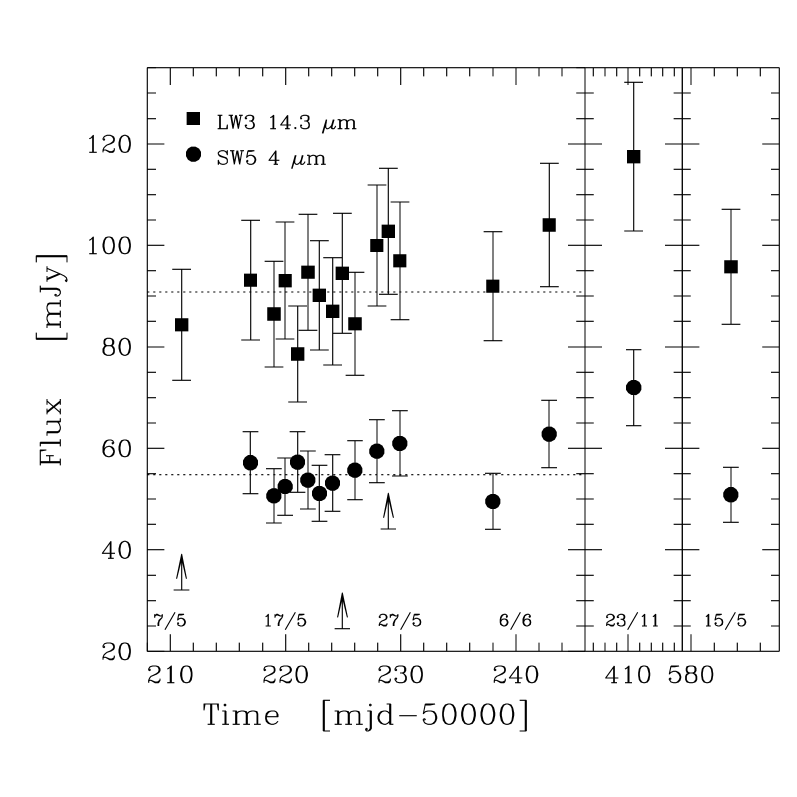
Figure 1: ISOCAM light curves of PKS 2155–304. The dotted curves represent the fitted constant of the best sampled period, from 1996 May 13 to May 27. The upward arrows are the lower limits in the SW5 curve.

Figure 2: ISOPHOT light curves of PKS 2155–304. The dotted curves represent the fitted constant curves of the best sampled period, from 1996 May 13 to May 27.

When the purpose is to verify whether the flux is variable, the contribution of the pixel responsitivity to the absolute error can be neglected and a smaller uncertainty can be associated to the relative flux values of the light curves. However, this can be done only for the two light curves of the photometer (see Tab. 5), due to the way the photometric error was determined.

The relative errors on the flux are, in any case, quite large, about 10 – 12% for the camera observations and from 20 to more than 50% for the photometer (see Appendix A). Within these uncertainties the light curves show no evidence of variability. To quantify this statement, we fitted the light curves with a constant term and the reduced chi–square values were computed in order to test the goodness of the fits. We first fitted the values of the best sampled period, from 1996 May 13 to May 27. The results are $54.8\pm 1.8$ mJy at 4.0 $\mu$m, $90.8\pm 3.2$ mJy at 14.3 $\mu$m, $315\pm 27$ mJy at 60 $\mu$m and $250\pm 34$ mJy at 90 $\mu$m. To fit the data at 4.0 $\mu$m the lower limits were neglected. We then repeated the fits, taking the mean of the above–mentioned period and adding the other data, to look for possible longer–term variability. All the fits are acceptable within a confidence level of 95%. This means that PKS 2155–304 showed no evidence of variability at these wavelengths in the observed period.

However, the large uncertainty on the flux can hide smaller variations. We calculated the mean relative error and obtained 3 sigma limits for the lowest detectable variations of 32%, 36%, 76% and 132% at 4.0, 14.3, 60 and 90 $\mu$m, respectively.

3.2 The infrared spectrum

The infrared spectral shape of PKS 2155–304 was sampled, using 16 filters, from 2.8 to 170 $\mu$m. The photometer filter C2_200 was not considered reliable enough and its observation was discarded. The flux values are given in Tab. 6 and the spectrum is shown in Fig. 3, in a $\log{\nu}-\log{\nu F(\nu)}$ representation.

Table 6: Fluxes of the observation of 1996 May 27, plus the upper limit at 170 $\mu$m.

ISO spectrum
filter	$\lambda$		$\nu$	flux					flux${}_{AAR}^{(a)}$
	$\mu$m		Hz	mJy					mJy
SW4	2	.8	$1.07\times 10^{14}$	32	.5	$\pm$	7	.0	38.2 $\pm$	3.1
SW2	3	.3	$9.08\times 10^{13}$	13	.0	(b)			28.3 $\pm$	5.6
SW6	3	.7	$8.10\times 10^{13}$	49		$\pm$	10		42.1 $\pm$	2.4
SW11	4	.26	$7.04\times 10^{13}$	64	.7	$\pm$	9	.3	52.8 $\pm$	5.5
SW10	4	.6	$6.52\times 10^{13}$	66		$\pm$	14		57.1 $\pm$	3.9
LW4	6	.0	$5.00\times 10^{13}$	33	.4	(b)			57.1 $\pm$	2.8
LW6	7	.7	$3.89\times 10^{13}$	44	.7	(b)			61.5 $\pm$	2.6
LW7	9	.6	$3.12\times 10^{13}$	66	.7	(b)			80.6 $\pm$	2.4
LW8	11	.3	$2.65\times 10^{13}$	84		$\pm$	17		122.0 $\pm$	3.7
LW9	14	.9	$2.01\times 10^{13}$	80	.6	$\pm$	8	.6	83.0 $\pm$	3.1
P2_25	25		$1.20\times 10^{13}$	88		$\pm$	11
C1_60	60		$5.00\times 10^{12}$	286		$\pm$	72
C1_70	80		$3.75\times 10^{12}$	184		$\pm$	59
C1_90	90		$3.33\times 10^{12}$	213		$\pm$	83
C1_100	100		$3.00\times 10^{12}$	172		$\pm$	72
C2_160	170		$1.76\times 10^{12}$	1235		(c)
(a) the automatic analysis results (OLP v6.3.2) are used to
compute the photometric error (see text)
(b) 1$\sigma$ lower limit
(c) 3$\sigma$ upper limit

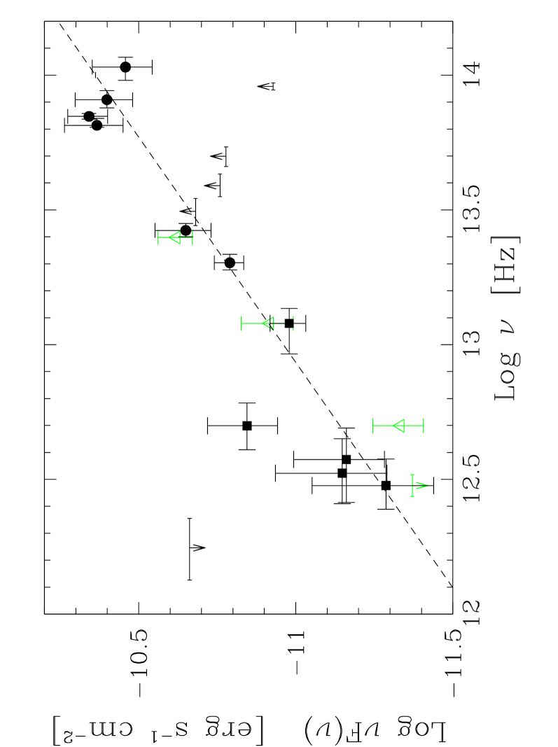
Figure 3: ISO spectrum. The dashed curve represents the power law fit. Circles are the ISOCAM data; squares are the ISOPHOT data. The horizontal bars indicate the filter width energy response. The upward arrows are the ISOCAM lower limits. The downward arrow at $\log{\nu}\sim 12.2$ is the ISOPHOT upper limit at 170 $\mu$m. Open triangles are the IRAS data (Impey & Neugebauer ImpeyNeugebauer (1988)) at 12, 25 and 60 $\mu$m; the IRAS upper limit at 100 $\mu$m is partially hidden.

In Fig. 3 it is also shown the result of a power law fit, that gives an energy spectral index of $\alpha=0.40\pm 0.06$. The lower and upper limits were not considered in the fit; the reduced chi–square is $\chi^{2}_{r}=1.31$, with 9 d.o.f., that gives a confidence level of 77.4%.

From each simultaneous pairs of flux values of the SW5 and LW3 light curves, we obtained the spectral indices between 4.0 and 14.3 $\mu$m as $\alpha_{i}=-\log(f_{SW5,i}/f_{LW3,i})/\log(\nu_{SW5}/\nu_{LW3})$. The mean value is $\alpha=0.403\pm 0.017$, which is fully consistent with the index derived using 11 filters on a larger IR band.

The fit with a constant term of the spectral indices $\alpha_{i}$ vs. time has a reduced chi–square of 0.26, with 13 d.o.f., which corresponds to a confidence level of less than 1%. This indicates that the source showed no spectral variability in the 4.0 – 14.3 $\mu$m range, during the observed period.

4 Optical observations

4.1 Observations and data reduction

The optical data were obtained using the Dutch 0.9 m ESO telescope at La Silla, Chile, between May 17 and 27 1996. The telescope was equipped with a TEK CCD 512x512 pixels detector and Bessel BVR filters were used for the observations. The pixel size is 27 $\mu$m and the projected pixel size in the plane of the sky is 0.442 arcsec, providing a field of view of 3^′.77 x 3^′.77.

The original frames were flat fielded and bias corrected using MIDAS package and photometry was performed using the Robin procedure, developed at the Torino Observatory, Italy, by L. Lanteri. This procedure fits the PSF with a circular gaussian and evaluates the background level by fitting it with a 1st order polynomial surface. The magnitude of the object and the error are derived by comparison with reference stars in the same field of view. The typical photometric error is $\sim 0.02$ mag in all bands.

4.2 Results

The light curves (Tab. 7 and Fig. 4) show an increase of luminosity of about 20% ($\sim 0.2$–$0.25$ mag), between the starting low level of May 17–18 and the maximum of May 24. The flux is then decreasing during the last two days. The behavior is very similar in all of the three filters.

Assuming that the optical spectrum is described by a power law, we calculated the mean spectral indices using the simultaneous pairs data of the light curves. The results are $\alpha_{RV}=0.62\pm 0.02$ and $\alpha_{VB}=0.60\pm 0.02$ and indicate that the optical spectrum is steeper than the IR one.

Table 7: RVB light curves.

obs. time		R	V	B
yy/mm/dd	mjd–50000	mag	mag	mag
96/05/17	220.4250	12.83	…	…
	220.4277	…	13.12	…
96/05/18	221.4298	…	…	13.45
	221.4354	…	13.12	…
96/05/23	226.4146	…	12.95	…
	226.4160	…	…	13.26
96/05/24	227.3625	12.62	…	…
	227.3660	…	12.90	…
	227.3688	…	…	13.21
96/05/26	229.4396	12.67	…	…
	229.4409	…	12.95	…
	229.4417	…	…	13.26
96/05/27	230.4194	12.78	…	…
	230.4202	…	13.06	…
	230.4215	…	…	13.38
Note: for all bands uncertainties are $\sim 0.02$ mag

Figure 4: Optical light curves of PKS 2155–304.

5 Discussion

5.1 IR flux and spectral variability

The ISO light curves of May–June 1996 show that the time variability of PKS 2155–304 in the mid– and far–infrared bands is very low or even absent. The flux has not varied significantly in 1996 November and in 1997 May, one year later, and is quite similar to the 1983 IRAS state (Impey & Neugebauer ImpeyNeugebauer (1988)) (Fig. 3), except at 60 $\mu$m, where the IRAS flux seems significantly lower. This agreement could support the idea that the infrared flux level of this source is rather stable. We have to wait for future satellite missions to test this statement.

The infrared spectrum from 2.8 to 100 $\mu$m is well fitted by a single power law. This is a typical signature of synchrotron radiation, that can explain the whole emission in this wavelength range, excluding important contributions of thermal sources.

The variability in the optical bands is small too, while the simultaneous RXTE light curve (Urry et al. Urry98 (1998), Sambruna et al. (1999)) shows, on the contrary, strong and fast variability at energies of 2–20 keV: the flux varied by a factor 2 on a timescale shorter than a day. This seems to be a common behavior in blazars, for which there is a more pronounced variability at frequencies above the synchrotron peak (Ulrich et al. (1997)).

5.2 Contribution of the host galaxy to the IR flux

The absence of variability could be also explained by the contribution, in the IR, of a steady component, such as the host galaxy. The host galaxy of PKS 2155–304 is a large elliptical which is well resolved in near infrared images (Kotilainen et al. (1998)), but the pixel field of view of the ISOCAM camera (3″or 6″) is too big to resolve it and its contribution is integrated in the flux of the active nucleus.

The magnitude of the host galaxy in the $H$ band is $m_{H}=12.4$ (Kotilainen et al. (1998)). The color of a typical elliptical at $z=0.11$ is $B-H$=4.6 (Buzzoni (1995)), from which we get $m_{B}=17.0$, which corresponds to a flux $f_{B}$ = 0.7 mJy. Mazzei & De Zotti (MazzeiDeZotti (1994)) calculated the flux ratio between the IRAS and the $B$ bands for a sample of 47 elliptical galaxies: their results are $\log{f_{12}/f_{B}}=0.01\pm 0.05$, $\log{f_{25}/f_{B}}=-0.70\pm 0.32$, $\log{f_{60}/f_{B}}=-0.22\pm 0.155$, $\log{f_{100}/f_{B}}=0.25\pm 0.10$. From these relations we can estimate the host galaxy fluxes in the far–IR at 12, 25, 60 and 100 $\mu$m: we have $f_{12}=0.7$ mJy, $f_{25}=0.1$ mJy, $f_{60}=0.4$ mJy, $f_{100}=1.2$ mJy. If we compare these values with those of Tab. 6, we see that they are less than 1% of the active nucleus flux, and much less than the uncertainties. We thus conclude that the contribution of the host galaxy to the ISO far–IR flux is negligible.

This fact can be also inferred from the spectral energy distribution (SED), built with the simultaneous data of May 1996 (Fig. 5), that shows that the ISO data lie on the interpolation between radio and optical spectra.

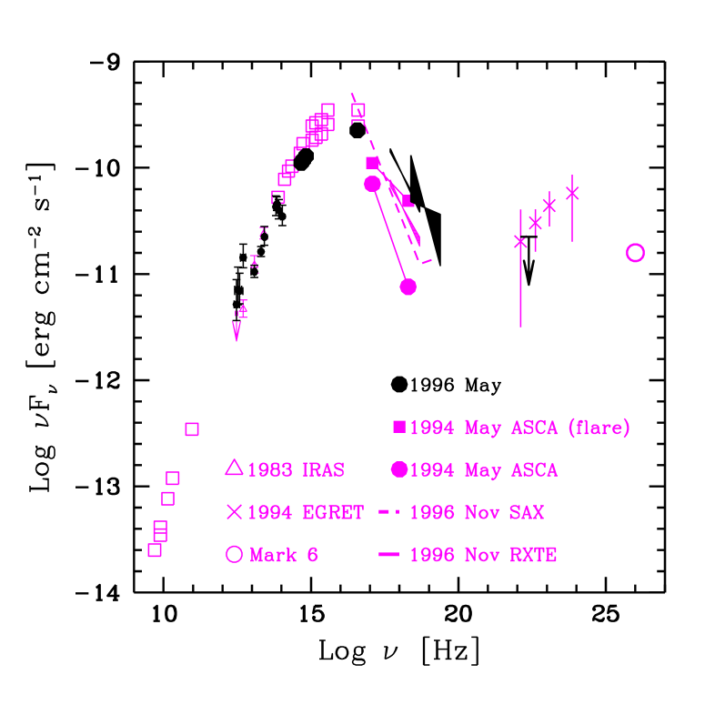
Figure 5: Spectral energy distribution of PKS 2155–304. The black data are the simultaneous data of 1996 May: circles are ISO and BVR fluxes (this paper, data of May 27), and EUVE flux (Marshall H.L., priv. comm.); the X–ray spectra are from RXTE (Urry et al. Urry98 (1998)); the $\gamma$–ray upper limit is from EGRET (Vestrand W.T., priv. comm.). Open grey boxes are data from the multiwavelength campaign of 1994 May (Pesce et al. Pesce (1997), Pian et al. Pian (1997), Urry et al. Urry97 (1997)). 1994 ASCA data are from Urry et al. (Urry97 (1997)), 1994 EGRET data are from Vestrand et al. (Vestrand (1995)), 1996 SAX spectrum is from Giommi et al. (Giommi (1998)), 1996 November RXTE spectrum is from Urry et al. (Urry98 (1998)), IRAS data are from Impey & Neugebauer (ImpeyNeugebauer (1988)), Mark 6 point is from Chadwick et al. (Chadwick (1999)).

5.3 Synchrotron self–absorption

The observed IR spectrum is rather flat, and one can wonder if this is due to a partially opaque emission, i.e. if we have, in the IR, the superposition of components with different self–absorption frequencies, as for the flat radio spectra.

To show that this is $not$ the case, we calculate the self–absorption frequency assuming that the IR radiation originates in the same compact region responsible for most of the emission, including the strongly variable X–ray flux. This is a conservative assumption, since the more compact is the region, the larger is the self–absorption frequency. In the case of an isotropic population of relativistic electrons with a power–law distribution $N(\gamma)=K\gamma^{-p}$, the self–absorption frequency is given by (e.g. Krolik 1999)

$$\nu_{t}={\delta\nu_{B}\over 1+z}\,\left[{3^{p\over 2}\pi\sqrt{3\pi}\over 4}\,{\Gamma({3p+22\over 12})\Gamma({3p+2\over 12})\Gamma({p+6\over 4})\over\Gamma({p+8\over 4})}\,{e\tau\over B\sigma_{T}}\right]^{\frac{2}{p+4}},$$

where $\Gamma$ is the gamma function, $\nu_{B}$ is the cyclotron frequency, $\delta$ is the beaming factor, $R$ is the size of the source, $\tau\equiv\sigma_{T}KR$, and $p$ is the slope of the electron distribution appropriate for those electrons radiating at the self–absorption energy. In the homogeneous synchrotron self–Compton model, the optical depth $\tau$ is approximately the ratio of the Compton and synchrotron flux at the same frequency. This ratio can be estimated from the SED (Fig. 5), where the Compton flux is obtained by extending at low frequencies the Compton spectrum with the same spectral index of the synchrotron curve. The upper limit for the $\gamma$–ray emission in 1996 May corresponds to an upper limit for the value of the optical depth of $\tau\lesssim 10^{-5}$. From the ISO spectrum, we have $p=2\alpha+1=1.8$. Although we cannot a priori determine the other two parameters, namely $B$ and $\delta$, a reasonable estimate can be derived through the broad band model fitting. In particular if we adopt the values derived by Tavecchio et al. (Tavecchio (1998)), $B=0.25$ G and $\delta\sim 30$, we get $\nu_{t}\lesssim 1.4\times 10^{11}$ Hz. For less extreme values of $\delta$, $\nu_{t}$ becomes smaller, while much larger values of the magnetic field (making $\nu_{t}$ to increase) are implausible, if the significant $\gamma$–ray emission is due to the self–Compton process, which requires the source not to be strongly magnetically dominated. The frequency of self–absorption is thus significantly lower then the IR frequencies, implying that the IR emission is completely thin.

5.4 Spectral energy distribution

In Fig. 5 we show the SED of PKS 2155–304 during our multiwavelength campaign, from the far IR to the $\gamma$–ray band. We also collected other, not simultaneous, data from the literature, especially in the X–ray band, to compare our overall spectrum with previous observations. As can be seen, our IR data fill a hole in the SED and, together with our optical results, contribute to a precise definition of the shape of the synchrotron peak. It is remarkable that although the X–ray state during our campaign was very high (one of the highest ever seen), the optical emission was not particularly bright. Also the upper limit in the $\gamma$–ray band testifies that the source was not bright in this band.

All this can be explained assuming that the X–ray flux is due to the steep tail of an electron population distributed in energy as a broken power law. The first part of this distribution is flat and steadier than the high energy, steeper part. In this case without changing significantly the bolometric luminosity large flux variations are possible above the synchrotron (and the Compton) peak. An electron distribution with these characteristics can be obtained by continuous injection and rapid cooling (see e.g. Ghisellini et al. (1998)). In fact, if the electrons are injected at a rate $Q(\gamma)\propto\gamma^{-s}$ between $\gamma_{1}$ and $\gamma_{2}$, the steady particle distribution will be $N(\gamma)\propto\gamma^{-(s+1)}$ above $\gamma_{1}$, and $\propto\gamma^{-2}$ below, until radiation losses dominate the particle escape or other cooling terms (e.g. adiabatic expansion). Electrons with energy $\gamma_{1}m_{e}c^{2}$ are the ones responsible for the emission at the synchrotron and Compton peaks (as long as the scattering process is in the Thomson limit). Since it is possible to change $s$ without changing the total injected power, large flux variations above the peak are compatible with only minor changes below. This model also predicts that the spectrum below the peak has a slope $\alpha=0.5$, which is not far from what we have observed in the far IR.

Appendix A Data reduction

A.1 ISOCAM

The observations were processed with CIA v2.0.

Each observation consisted in a sequence of frames, which had an elementary integration time of about 2 s. By this way the temporal behaviour of each pixel was known.

First, the dark current was subtracted from each raw frame, using the dark images present in the software library, flagging the bad pixels of SW and LW detectors.

The impact of charged particles (glitches) on the detectors create spikes in the pixel signal curve. To remove these spurious signals, we first used the Multiresolution Median Transform method (Starck et al. (1996)), then every frame was inspected to make sure that the number of suppressed noise signals was negligible and finally a manual deglitching operation was done to detect the glitches left and flag them. Some glitches caused a change in the pixel sensitivity: in this case we flagged the pixel in all readouts after the glitch.

The library dark images were not good enough to remove all the effects of the dark current: the signals in rows and columns showed a saw–teeth structure, that was eliminated using the Fast Fourier Transform technique (Starck & Pantin (1996)).

The response of the detector pixels to a change in the incident flux is not immediate and the signal reaches the stabilization after some time. This time interval depends on the initial and final flux values and on the number of readouts (ISOCAM Observer’s Manual (1994)). Therefore, the time sequence of a pixel signal shows, after a change in the incident flux, an upward or downward transient behaviour. At the beginning of every observation, after a certain number of frames, the signal should reach the stable value. As this ideal situation could not always been achieved, CIA provides different routines to overcome this problem and apply the transient correction. These routines use different models to fit the signal curves, in order to identify the stable value.

In the SW5 observations, the photons coming from PKS 2155–304 fell mainly in one or two pixels, whose signals showed an upward transient behaviour that never reached the stabilization. On the contrary, the background, being very low, was stabilized. No transient correction routines were able to adequately fit the source signals, either underestimating or overestimating the stable flux. Observing the signal curves, we noticed that the behaviour of the first part of the curves were far from the expected converging trends that are used in the models of the correction routines, while the remaining part of the curves seemed to be well described by a converging exponential trend. So, after having discarded the starting readouts, we fitted the signal with a simple exponential model $s_{fit}=s_{\infty}+c\cdot e^{-t/\tau}$, where the optimized parameters are $c$, $\tau$ and $s_{\infty}$, that represents the stable signal. We chose the fit which showed a reasonable result and optimized the determination coefficient $R^{2}=1-\frac{\sum_{i}(s_{i}-s_{fit})^{2}}{\sum_{i}(s_{i}-\bar{s})^{2}}$, where $s_{i}$ are the measured signals and $\bar{s}$ is the mean of the part we considered. In three cases, the results were not acceptable and we could define only lower limits, as the upward transients had not reached the stabilization.

For the transient correction of the LW3 observations, the model developed at the Institut d’Astrophysique Spatiale (IAS Model) (Abergel et al. (1996)) has been used. As the corrected curves attained stable values in the second half only, we did not use the first half of the frames.

In the spectral observation of May 27, the uninterrupted sequence of filters used created either upward or downward transients and the stabilization of the source signal was reached just in few cases. The five observations made with the SW channel were corrected using the same method as the SW5 ones, except for the SW11 filter, in which the stabilization was reached for all pixels. In this case, we just discarded the first half of the 162 frames. In the SW2 filter data, at the end of the observation, the source signal was so far from stabilization that we could define only a lower limit. The five observations made with the LW channel were corrected using the IAS model. As this model takes into account all the past illumination history, we fitted a unique curve that was built linking together all the LW filters data. This method worked fine for two filters only (LW8 and LW9), while for the other three filters again we defined lower limits.

We averaged all the frames neglecting the flagged signal values and then the images were flat fielded, using the library flat fields of CIA.

The total signal of the source was computed integrating the values of the signal in a box centered on the source and subtracting the normalized background obtained in a ring of 1 pixel width around the box. The boxes had dimension ranging from 3x3 to 7x7 pixels, depending on the filter and on the pixel field of view (pfov). The results were colour corrected and divided for the point spread function (PSF) fraction falling in the box. This fraction also depends on filters and pfov. To compute it, we extracted from the library, for each combination of filter and pfov, the nine PSF images centered more or less on the same pixels of PKS 2155–304. For calibration requirements, in each PSF image the centroid of the source was placed in a slightly different position inside the same pixel. As we do not know with enough accuracy the position of the centroid of PKS 2155–304 in the ISOCAM images, the nine PSF were averaged and the result was normalized. The PSF correction was calculated by summing the signal of the pixels in a box of the same dimension of that in which we extracted the source signal. For the LW detector, a further correction factor was applied to take into account the flux of the point–like source that falls outside the detector (Okumura (1997)). For the SW channel, we adopted for all filters the SW5 PSF, because, along with SW1, was the only one present in the calibration library, however the error we introduced can only be of a few percent.

Finally, the source signal was converted to flux density using the coefficients in Blommaert (Blommaert (1997)).

To compute the photometric error we divided the uncertainty sources in two parts: the first one took into account the dark current subtraction, deglitching, flat fielding operations and signal to flux conversion, while the second one considered the transient correction. The first group of error sources are derived from the Automatic Analysis Results (AAR; OLP v7.0 for the light curves data, OLP v6.3.2 for the spectrum data). The source flux values $f_{AAR}$ given by the AAR are not reliable because the transient correction is not performed, but the AAR absolute flux errors $\sigma_{AAR}$ are a good estimate of the first group of errors (the AAR fluxes are given in Tabs. 4 and 6). We assumed that the fluxes $f_{src}$ that we derived have the same relative error $\sigma_{rel}=\sigma_{AAR}/f_{AAR}$. Thus, for our fluxes this part of error is $\sigma_{f}=\sigma_{rel}\,f$, which accounts for all the uncertainties sources, but the transient correction. We estimated that the error due to the transient correction is of the order of 10%, which is the rounded maximum error on the stable signal $s_{\infty}$, obtaining a total error of $\sigma=\sqrt{\sigma^{2}_{f}+\sigma^{2}_{tr}}$. We assumed then a $\sigma_{tr}$ of 10% for all our measurements (20% for SW4 and SW10 filters).

A.2 ISOPHOT

The observations were done in rectangular chopped mode: the observed field of view switches alternately between the source and an 180″ distant off–source position. This is necessary in order to measure the background level. The chopping direction was along the satellite Z-axis, which was slowly rotating by about one degree per day. Thus, every time the background was sampled in different fields of the sky and a raster map was performed just to check the stability of the background all around the source. The standard deviation of the background flux measured in the central pixel of the C100 detector, in the eight off-source positions of the scan, is 37 mJy. This value is much less than the error of the source flux (see Tab. 5). This small background fluctuation would lead to a rise of the scatter of the source flux, in any case our results are compatible with absence of variability (see section 3).

Each observation of an astronomical target was immediately followed by a Fine Calibration Source (FCS) measurement, using internal calibrations sources. These measurements were made in order to determine the detector responsitivity, which is necessary to compute the target flux.

Each observation consisted in a series of integration ramps, each one made by the sequence of voltage readouts between two destructive readouts.

The observations were processed with PIA v7.0 (Gabriel et al. (1997)).

PIA separates the operations to be performed on the data in different levels: at each level PIA creates a data structure on which it operates. This data structure takes its name according to the properties of the data. The first part of the data analysis was common for all the observations, then the procedures changed according to the different characteristics of the observation (whether it was chopped or not or whether the detector was receiving photons from the astronomical target or from the FCS).

At the beginning, PIA automatically converted the digital data from telemetry in meaningful physical units and created the structure of data, called Edited Raw Data (ERD). At the ERD level, some starting readouts and the last readout of each ramp were discarded, because they are disturbed by the voltage resetting; we also manually discarded the part of the ramp before or after a glitch (that causes a sudden jump of the readout value) in the cases where most part of the ramp was unchanged and the glitch did not modify the detector responsitivity. A correction for the non–linear responsitivity of the detector was applied, using special calibration files. Then, each ramp was fitted by a 1st order polynomial model. A signal (in V s^-1) was obtained from the slope of every ramp: the slope is proportional to the incident power. At Signal per Ramp Data (SRD) level, the first half of the signals per chopper plateau were discarded, because of stabilization problems. As the signal value depends on the integration time, a correction factor was applied and the signal was normalized for an integration time of 1/4 s. The dark current was subtracted using the PIA calibration files, which take into account the satellite position in the orbit. An algorithm was applied to discover and discard the signals that were anomalously high, because of glitches; then, the signals of each chopper plateau were averaged. At Signal per Chopper Plateau (SCP) level, the responsitivity of each detector pixel was computed taking the median of the FCS2 signals of the calibration measurements; then, the vignetting correction was performed on the target observations. In the chopped measurements, the background, that was calculated at the off–source position, was subtracted to get the source signal.

As for the camera, the response of the photometer detectors has some delays after a change in the incident flux. This effect causes losses in the signal values measured in the chopped measurements, so a correction factor was applied. The signal was finally converted into power, using the responsitivity obtained from the FCS measurement.

In the observations performed with the 3x3 pixel C100 detector, only the central pixel was used to compute the source flux density, because, as the most of the Airy disk of a point-like source centered in the pixel lies in the same pixel (69% for C1_60 and 61% for C1_90), to use the outer pixels just adds more noise than signal. The source flux density is defined as $F_{\lambda}=P_{src}/(C1f_{psf})$, where $P_{src}$ is the incident power, $C1$ is a conversion factor of each filter (as given in the PIA calibration file pfluxconv.fits) and $f_{psf}$ is the fraction of PSF that falls on the pixel considered when the source is located in the centre (ISOPHOT Observer’s Manual (1994), Tabs. 2 and 4).

The absolute photometric error was computed by PIA, during the data reduction process, and took into account the uncertainty in the determination of the slope of the ramp and the errors associated to the other performed correction operations.

References

- Abergel et al. (1996) Abergel A., Désert F.X. & Aussel H., 1996, IAS model for ISOCAM LW transient correction, v1.0, November 1996, Technical Report
- (2) Blommaert J., 1997, ISOCAM Photometry Report, September 1997, Technical Report
- Buzzoni (1995) Buzzoni A., 1995, ApJS, 98, 69
- Césarsky et al. (1996) Césarsky C.J., Abergel A., Agnèse P., et al., 1996, A&A 315, L32
- (5) Chadwick P.M., Lyons K., McComb T.J.L., et al., 1999, ApJ 513, 161
- (6) Edelson R., Krolik J., Madejski G., et al., 1995, ApJ 438, 120
- Gabriel et al. (1997) Gabriel C., et al., 1997, The ISOPHOT Interactive Analysis PIA, a calibration and scientific analysis tool, in Proc. of the ADASS VI conference, ASP Conf.Ser., Vol.125, eds. G. Hunt & H.E. Payne, p108
- Ghisellini et al. (1998) Ghisellini G., Celotti A., Fossati G., Maraschi L. & Comastri A., 1998, MNRAS, 301, 451
- (9) Giommi P., Fiore F., Guainazzi M., et al., 1998, A&A 333, L5
- (10) Impey C.D. & Neugebauer G., 1988, AJ 95, 307
- ISOCAM Observer’s Manual (1994) ISOCAM Observer’s Manual, 1994, The ISOCAM Team and A. Heske, available at http://www.iso.vilspa.esa.es/manuals/iso_cam/
- ISOPHOT Observer’s Manual (1994) ISOPHOT Observer’s Manual, 1994, The ISOPHOT Consortium, eds. U. Klaas, H. Krüger, I. Heinrichsen, A. Heske and R. Laureijs, ESA
- Kotilainen et al. (1998) Kotilainen J.K., Falomo R. & Scarpa R., 1998, A&A 336, 479
- (14) Krolik J.H., 1999, in Active Galactic Nuclei: from the Central Black Hole to the Galactic Environments, Princeton Series in Astrophysics, Princeton University Press (New Jersey), p.279
- Kessler et al. (1996) Kessler M.F., Steinz J.A., Anderegg M.E., et al., 1996, A&A 315, L27
- Lemke et al. (1996) Lemke D., Klaas U., Abolins J., et al., 1996, A&A 315, L64
- (17) Mazzei P. & De Zotti G., 1994, ApJ 426, 97
- Okumura (1997) Okumura K., 1997, ISOCAM PSF Report, September 1997, Technical Report
- Padovani & Giommi (1995) Padovani P. & Giommi P., 1995, ApJ 444, 567
- (20) Pesce J.E., Urry C.M., Maraschi L., et al., 1997, ApJ 486, 770
- (21) Pian E., Urry C.M., Treves A., et al., 1997, ApJ 486, 784
- Sambruna et al. (1999) Sambruna et al., 1999, in preparation
- Starck & Pantin (1996) Starck J.L. & Pantin, E., 1996, Second Order Dark Correction, v1.0, March 1996, Technical Report, CEA Saclay
- Starck et al. (1996) Starck J.L., Claret A. & Siebenmorgen R., 1996, ISOCAM Data Calibration, v1.0, March 1996, C.E.A. Technical Report
- (25) Tavecchio F., Maraschi L. & Ghisellini G., 1998, ApJ 509, 608
- Ulrich et al. (1997) Ulrich M.–H., Maraschi L. & Urry C.M., 1997, ARA&A, 35, 445
- (27) Urry C.M., Treves A., Maraschi L., et al., 1997, ApJ 486, 799
- (28) Urry C.M., Sambruna R.M., Brinkmann W.P. & Marshall H., 1998, in: Scarsi L., Bradt H., Giommi P., Fiore F. (eds.) The Active X–Ray Sky. Nucl. Phys. B (Proc. Suppl.) 69, 419
- (29) Vestrand W.T., Stacy J.G. & Sreekumar P., 1995, ApJ 454, L93