The Distribution of Stellar Orbits in the Giant Elliptical Galaxy NGC 2320

Abstract

We present direct observational constraints on the orbital distribution of the stars in the giant elliptical NGC 2320. Long-slit spectra along multiple position angles are used to derive the stellar line–of–sight velocity distribution within one effective radius. In addition, the rotation curve and dispersion profile of an ionized gas disk are measured from the [OIII] emission lines. After correcting for the asymmetric drift, we derive the circular velocity of the gas, which provides an independent constraint on the gravitational potential.

To interpret the stellar motions, we build axisymmetric three–integral dynamical models based on an extension of the Schwarzschild orbit–superposition technique. We consider two families of gravitational potential, one in which the mass follows the light (i.e., no dark matter) and one with a logarithmic gravitational potential.

Using $\chi^{2}$–statistics, we compare our models to both the stellar and gas data to constrain the value of the V-band mass–to–light ratio $\Upsilon_{V}$. We find $\Upsilon_{V}=15.0\pm 0.6$ $h_{75}$ for the mass-follows-light models and $\Upsilon_{V}=17.0\pm 0.7$ $h_{75}$ for the logarithmic models. For the latter, $\Upsilon_{V}$ is defined within a sphere of $15^{\prime\prime}$ radius.

Models with radially constant $\Upsilon_{V}$ and logarithmic models with dark matter provide comparably good fits to the data and possess similar dynamical structure. Across the full range of $\Upsilon_{V}$ permitted by the observational constraints, the models are radially anisotropic in the equatorial plane over the radial range of our kinematical data ($1^{\prime\prime}\mathrel{\hbox to0.0pt{\lower 3.0pt\hbox{$\sim$}\hss}\raise 2.0pt\hbox{$<$}}r\mathrel{\hbox to0.0pt{\lower 3.0pt\hbox{$\sim$}\hss}\raise 2.0pt\hbox{$<$}}40^{\prime\prime}$). Along the true minor axis, they are more nearly isotropic. The best fitting model has $\sigma_{r}/\sigma_{\rm total}\simeq 0.7$, $\sigma_{\phi}/\sigma_{\rm total}\simeq 0.5-0.6$ and $\sigma_{\theta}/\sigma_{\rm total}\simeq 0.5$ in the equatorial plane.

1 Introduction

The orbital distribution of stars, often quantified by the (an)–isotropy of the local velocity dispersion, is a useful measure of the dynamical state of a galaxy. It provides constraints on galaxy formation and helps discriminating between N-body merger remnants. Furthermore, it has been a classic diagnostic to study the mass distribution of galaxies.

Anisotropy profiles can only be obtained from observations through a dynamical model, since only line–of–sight velocities can be measured for external galaxies. For a number of reasons the construction of such models is more difficult for elliptical galaxies than for spirals. Elliptical galaxies generally have no simple tracer population that could be used to derive the underlying gravitational potential (like HI disks in spirals). These systems are known to support a variety of orbital shapes that largely overlap each other. Furthermore different orbit distributions and gravitational potentials may result in very similar observable kinematics, known as the mass–anisotropy degeneracy. On the observational side, stellar velocity distributions in ellipticals usually have to be derived from absorption lines, which limits the maximal radius for kinematics.

This situation is improving on various fronts: fully anisotropic dynamical models can now be constructed and matched to observations (see e.g., Rix et al. 1997; Richstone et al. 1997; Gerhard et al. 1998; Cretton et al. 1999, hereafter C99; Gebhardt et al. 2000). The mass–anisotropy degeneracy can in principle be broken with the use of the full line–of–sight velocity distributions, also called Velocity Profiles (hereafter VPs) (see e.g., Dejonghe 1987; Gerhard 1993). Measurements of VPs at several position angles and extended radii further constrain the dynamical structure of the galaxy (see e.g., Carollo et al. 1995; Statler, Smecker–Hane & Cecil 1996).

As a consequence, information about the intrinsic dispersion profiles in elliptical galaxies is slowly emerging: spherical anisotropic models for NGC 2434 show $\sigma_{r}/\sigma_{\rm total}=0.7$, $\sigma_{\theta}/\sigma_{\rm total}=\sigma_{\phi}/\sigma_{\rm total}=0.5$. Matthias & Gerhard (1999) built axisymmetric 3–integral models of NGC 1600 (they did not need any DM inside 1 effective radius $\rm R_{eff}$, enclosing half of the light), deducing radial anisotropy in the outer parts ($\sigma_{\theta}/\sigma_{r}\simeq\sigma_{\phi}/\sigma_{r}\simeq 0.7$), and a more isotropic structure in the center. In their spherical models of NGC 6703, Gerhard et al. (1998) again found near isotropy in the center, and a mild radial anisotropy in the outer parts, as in NGC 1399 (Saglia et al. 1999). Dejonghe et al. (1996) inferred tangential anisotropy in NGC 4697, as in NGC 1700 (Statler et al. 1999) based on axisymmetric 3–integral models built with a quadratic programming technique, but no VPs were used in these two studies. Using fully general axisymmetric models, van der Marel et al. (1998) explored the orbital structure of the small rapidly rotating elliptical M32; using similar technique, Gebhardt et al. (2000; and in preparation) studied NGC 3379, NGC 3377, NGC 4473 and NGC 5845 and found that they were radially anisotropic in the range (0.1 - 1) $\rm R_{eff}$. Merritt & Oh (1987) derived a slight radial anisotropy $\sigma_{r}\simeq 1.2\sigma_{\phi}=1.2\sigma_{\theta}$ in the main body of M87, but they did not model the full VPs.

In this paper, we derive the anisotropy of the stellar orbits in the giant elliptical NGC 2320, combining constraints from the stellar VPs and from the gas rotation and dispersion curves. The simple kinematics of the gas (mainly circular rotation) allows an independent and straightforward measure of the total mass of the system. Cinzano & van der Marel (1994) constructed dynamical models for NGC 2974 and found that the velocities of the ionized gas disk were consistent with the potential derived from the stellar kinematics.

The paper is organized as follows. In Section 2, we present the photometric and kinematic data. We describe the mass and dynamical models in Section 3. The range of statistically acceptable models with their associate dynamical structure is derived in Section 4. Section 5 summarizes the results and discusses them in the context of cosmological simulations and mergers.

2 The data

2.1 Photometric data

NGC 2320 is a luminous elliptical galaxy with a heliocentric velocity of 5725 km/s, implying a distance of 76.3 $h_{75}$ Mpc. It has an apparent magnitude $m_{V}=11.9$ (NED), which translates to an absolute magnitude of ${\rm M}_{V}=-22.5$. A V-band image was obtained at the Steward Observatory $90^{\prime\prime}$ Telescope on March, 1996 with a 2k x 2k CCD and an exposure time of 600 seconds. The scale was 0.283 arcseconds per pixel. The image was calibrated using published aperture photometry available via the Hypercat catalogue (CRAL, Lyon), mostly consisting of data taken at the OHP (Prugniel & Heraudeau 1998). The effective radius $\rm R_{eff}$ is 29.5${}^{\prime\prime}$. Our photometric data is not good enough to detect a possible central luminosity cusp (the seeing was about 1${}^{\prime\prime}$) and no HST archive image exists. In this paper, however, we cannot concentrate on the core properties of NGC 2320, since we used a wide slit for the spectroscopic observations.

2.2 Stellar kinematic data

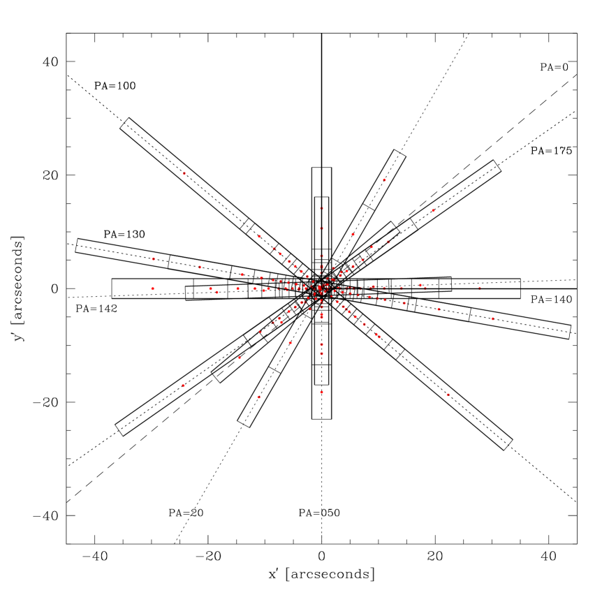
Figure 1: Position of all the slits used to constrain the dynamical models. The values of the various position angles are indicated (the major axis is PA=140 and the minor axis is PA=50). The effective radius $\rm R_{eff}$ is at $29.5^{\prime\prime}$.

NGC 2320 was observed during three different runs (February 96, February 98 and March 1998) at the Multi Mirror Telescope (MMT) and the 4 meter telescope at Kitt Peak. Table 1 summarizes the observations and Figure 1 illustrates all slit positions on the plane of the sky. All these various spectra are statistically independent constraints even if they have the same PAs, because they have a different radial extent (and binning) and, in some cases, have been obtained at a different telescope.

After standard reduction procedures with IRAF, the VPs were extracted from the absorption lines and quantified using the Gauss-Hermite decomposition (see e.g. Rix & White 1992, van der Marel & Franx 1993). With the same notation as in Cretton & van den Bosch (1999, hereafter CvdB99), we parameterize these velocity profiles (VPs) using Gauss-Hermite series with line strength $\gamma$, mean radial velocity $V$, and velocity dispersion $\sigma$ as free parameters. The anisotropy is reflected in the shape of the VPs (and hence in the values of the GH–moments $h_{i}$). Qualitatively, VPs more peaked than a Gaussian tend to originate from radial anisotropy and translate into greater $h_{4}$ values than their isotropic counterparts. Note that the VP shapes not only depend on the dynamical structure, but also on the gravitational potential, and can hence be used to break the mass–anisotropy degeneracy (Dejonghe 1987, Merritt 1993, Gerhard 1993, see also Figure 2 in Gerhard et al. 1998, Carollo et al. 1995). In total, we have 632 stellar kinematic constraints (158 data points $\times$ 4 GH–moments $h_{1,\ldots,4}$, see Table 1).

A careful look at the kinematic data (Figure 6) reveals some systematic uncertainties, e.g., the left/right assymetries. Also about half of the slits show a significantly higher ($\sim 40{\rm\,km\,s^{-1}}$) central dispersion value than for the remaining half. Given their formal errors ($\sim 10{\rm\,km\,s^{-1}}$), such large differences amongst various PAs can not be explained through statistical fluctuations and are probably due to the strong gradients inside the central pixel, since we use a wide slit. Therefore we decide to replace the formal error bars of the central velocity dispersions by the variance amongst the (central) dispersion values from different slit positions.

2.3 Kinematics of the ionized gas

After subtraction of the broadened stellar template, emission was found at 5007 [Å] and 4965 [Å], corresponding to the [OIII] lines of ionized gas (see e.g., Figure 2 of Rix et al. 1995). However, only the MMT data was of sufficient S/N to permit measurement of mean velocity and velocity dispersion.

Usually, gas is assumed to rotate in the equatorial plane of a galaxy on nearly closed orbits. However, this is only true if the velocity dispersion is negligible compared to the mean rotation velocity. In Figure 2, we show the mean line–of–sight velocity and dispersion of the gas on the MMT major axis: The velocity reaches 325 km/s (inside $20^{\prime\prime}$) and the dispersion decreases roughly exponentially from 220 km/s (center) to 100 km/s (at $15^{\prime\prime}$) and thus can not be neglected.

To derive the true circular velocity $v_{c}^{2}=R\;\partial\Phi_{\rm grav}/\partial R$ from the observed $v_{\rm gas}$ and $\sigma_{\rm gas}$, we proceed as follows (see e.g., Neistein et al. 1999). We first obtain the mean rotation velocity of the gas, $v_{\phi}(R)$, in the equatorial plane (i.e., the plane of the disk) by de-projecting the observed $v_{\rm gas}$. Along the major axis, we have $v_{\phi}(R)=v_{\rm gas}/{\rm sin}\,i$, where $i$ is the inclination of the galaxy (away from face–on). Similarly, we have $\sigma_{\phi}(R)=\sigma_{\rm gas}/{\rm sin}\,i$. Note that in nearly edge–on disks, this is only approximately true, since the line–of–sight integration through the disk will reduce $v_{\rm gas}$ relative to $v_{\phi}$. Neistein et al. (1999) estimated that this correction is less than 4% for inclinations $i<70^{\rm o}$.

We follow Binney & Tremaine (1987, eq. 4–33) to obtain the circular velocity of the cold gas disk:

$$v_{c}^{2}=\overline{v_{\phi}^{2}}+\sigma_{\phi}^{2}-\sigma_{R}^{2}-{R\over\rho}{\partial(\rho\sigma_{R}^{2})\over\partial R}-R{\partial(\overline{v_{R}v_{z}})\over\partial z},$$ (1)

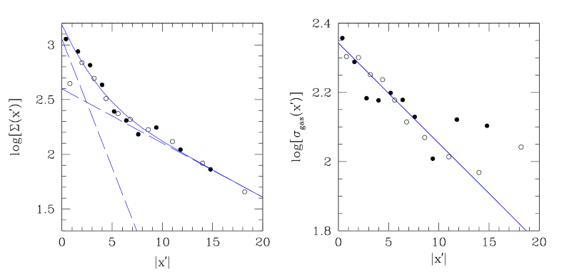
Figure 3: Surface density profile of the ionized gas disk (left) and dispersion profile (right) along the major axis. The dots are the measured quantities, the full line is the fit. On the left panel, the dashed lines are the individual exponentials. Both sides of the major axis are shown: full symbols correspond to the positive side and open symbols to the negative side of the major axis.

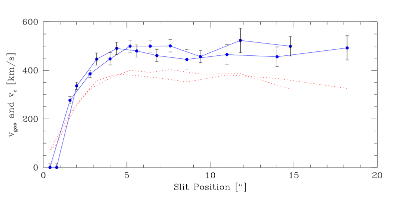
Figure 4: Circular velocity as a function of radius (full line) when the asymmetric correction has been applied. For comparison, we plotted also the observed gas velocity (dotted line). Both sides of the major axis have been folded to the positive side. Only points at radii larger than $3^{\prime\prime}$ should be taken seriously, since during the correction we have assumed a flat rotation curve.

where we assume that the final term can be neglected (i.e., the gas dynamics is close to isotropy). We fit the luminosity density of the gas as $\rho(R)=\rho_{1}\;{\rm exp}(-R/R_{1})+\rho_{2}\;{\rm exp}(-R/R_{2})$ as shown in the left panel of Figure 3. For a flat rotation curve, the epicycle approximation gives $\sigma_{R}^{2}(R)=2\sigma_{\phi}^{2}(R)$. Since the term $\sigma_{R}$ enters a derivative in eq. (1) we find it convenient to use an analytic expression instead of the (noisy) data points, so we fit an exponential to $\sigma_{\rm gas}(R)=\sigma_{0}\;{\rm exp}(-R/R_{0})=\sigma_{\phi}(R)\;{\rm sin}\,i$ (right panel in Figure 3). We can now evaluate the circular velocity (Figure 4). The error bars for $v_{c}(R)$ have been estimated from the left/right differences of the rotation curve.

3 The models

3.1 The mass model

As in CvdB99, we have used the Multi Gaussian Expansion (MGE) of Emsellem et al. (1994) to construct a mass model for NGC 2320. Briefly, in this formalism the surface brightness profile, the mass density distribution and the PSF are all described as a sum of Gaussian components. Free parameters include the center of each Gaussian, its position angle, flattening, central intensity, and size (i.e., standard deviation) along the major axis.

We find that the density profile of NGC 2320 can be well fitted with 5 Gaussian components (see Table 2), all with the same position angle and center. The mass density is expressed as

$$\rho(R,z)=\Upsilon\;\sum_{i=1}^{5}I_{i}\;{\rm exp}\Biggl{[}-{1\over 2\sigma_{i}^{2}}\biggl{(}R^{2}+{z^{2}\over q_{i}^{2}}\biggr{)}\Biggr{]},$$ (2)

where $\Upsilon$ is the mass–to–light ratio, $I_{i}$ is the central intensity (in ${\rm\,L_{\odot}}/{\rm arcsecond}^{3}$), $\sigma_{i}$ the standard deviation (in arcseconds) and $q_{i}$ the flattening of each Gaussian. The corresponding gravitational potential (and forces) are obtained by solving Poisson equation and can be written as one–dimensional quadratures (see CvdB99 for details). In this case, the mass distribution follows the light.

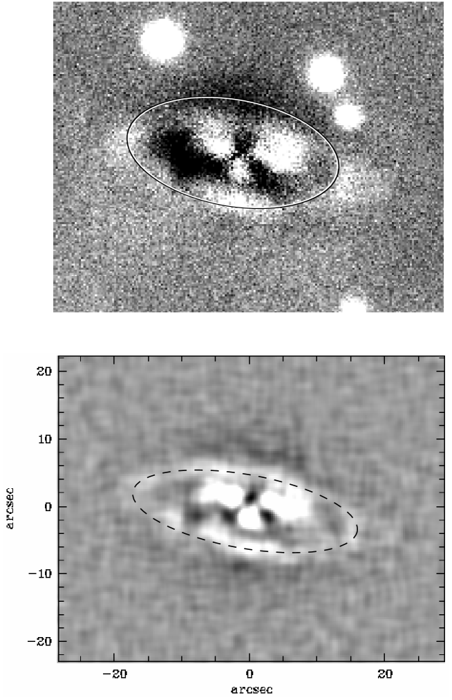
Figure 5: Ring–like structure once the MGE model has been subtracted from the image (top panel): an ellipse with an axis ratio of 0.5 is superposed (see text). The bottom panel shows an unsharp mask image with an ellipse of axis ratio of 0.32 (dashed line) that would translate into an inclination of $71^{\rm o}$. The big white dots outside the ring in the top panel are foreground stars.

When we subtract the MGE model from the image, a disky structure appears with a radial extent of $\sim 17^{\prime\prime}$. If we interpret this feature as a ring of young stars and dust (hence darker on the near side), we derive an axis ratio of 0.5 (top panel of Figure 5). After additional filtering (unsharp masking) a somewhat flatter ellipse of emission (with an axis ratio of 0.32 corresponding to an inclination of $71^{\rm o}$) appears (bottom panel of Figure 5). However, our main results are not strongly dependent on the precise choice of the inclination. For the remainder of this paper, we adopt an axis ratio of 0.5, which translates into an inclination $i=60^{\rm o}$. The apparent flattening of the galaxy (0.6–0.7) makes it unlikely to be much more inclined, since galaxies intrinsically as flat as E6 are very rare. Van den Bosch & Emsellem (1998) found a similar stellar ring in the nuclear region of NGC 4570.

We have explored another set of models in which the total gravitational potential and the luminous density are not related by Poisson equation: models with a logarithmic potential

$$\Phi_{\rm log}(R,z)={1\over 2}\,v_{0}^{2}\;{\rm ln}\Biggl{(}R_{c}^{2}+R^{2}+{z^{2}\over q_{\Phi}^{2}}\Biggr{)}.$$ (3)

We still use the MGE density law (equation 2) to describe the luminosity profile of NGC 2320. We have chosen the simple logarithmic potential (with flat circular velocity at large radii) to build a sequence of models with dark matter halos. We took $q_{\Phi}=0.83$ such that the flattening of the corresponding mass density profile is similar to that of the MGE models, $q_{\rho}\sim 0.5-0.6$. We adjust $R_{c}$ such as to match the inner parts of the circular velocity curve and we scale the various models with $v_{0}$. The quantity $R_{c}$ is probably an upper limit of the true core radius, since we did not fit deconvolved data. Nevertheless it is not likely to have a large influence on the main results of this paper.

In Rix et al. (1997), we used dark halo profiles suggested by cosmological N–body simulations (Navarro, Frenk, & White, 1996) and adiabatically contracted them to account for the luminous material. We found that the best fit dark halo profile was nearly indistinguishable from a simple logarithmic model over the radii probed by the kinematics of integrated light.

3.2 The dynamical models

We construct dynamical models based on the orbit superposition technique of Schwarzschild, described in detail in C99. Here, we limit ourselves to listing the specific parameters we used for NGC 2320: Starting with a ”trial potential”, $\Phi(R,z)$, we sample orbits on a grid in integral space, energy $E$, vertical component of the angular momentum $L_{z}$ and third integral $I_{3}$. We use 20 values of $E=1/2\;R_{c}\;\partial\Phi/\partial R+\Phi(R_{c},0)$, represented through the radius of the circular orbit $R_{c}(E)$. We space $R_{c}(E)$ logarithmically in $[0.1^{\prime\prime},300.0^{\prime\prime}]$, which encloses more than 99 % of mass for our MGE model. For each $E$, we adopt 14 values of $L_{z}$ in $[-L_{z,{\rm max}},+L_{z,{\rm max}}]$ and 7 values of $I_{3}$ per ($E,L_{z}$) were adopted as in CvdB99. We cannot assume that $I_{3}$ is defined for every value of ($E,L_{z}$), i.e., every orbit is regular. Instead we sample starting points on the zero–velocity curve (see C99); when the orbit is indeed regular, this starting point can truly be interpreted as a third integral, $I_{3}$.

The orbit library is constructed by numerical integration of each trajectory for a fixed amount of time, 200 periods of the circular orbit at that E, using a Runge–Kutta scheme. During integration, we store the fractional time spent by each orbit in a Cartesian data–cube of observables $(x^{\prime},y^{\prime},v_{\rm los})$, where $(x^{\prime},y^{\prime})$ are the projected coordinates on the sky and $v_{\rm los}$ is the line–of–sight velocity. This map is subsequently convolved with the PSF and binned to match the various slit apertures. Furthermore, we adopt logarithmic polar grids in the meridional plane $(R,z)$ and in the $(x^{\prime},y^{\prime})$ plane with the same $R_{c}$–radial range and sampling. Orbital occupation times are stored both on the intrinsic and projected grids to make sure the final orbit model reproduces (to a few percent accuracy) the MGE mass model. The lowest order velocity moments of each orbit are also stored on such a grid to analyze the dynamical structure of the resulting model (see C99 for details).

The mass on each orbit is determined from the non–negative superposition of all orbits that best reproduces the kinematic data within the errors and the projected and intrinsic MGE mass profile. Using the NNLS algorithm (Lawson & Hanson, 1974), smoothness in integral space is enforced through a regularization technique. It allows the derivation of smooth anisotropy profiles of a few selected models.

4 Results

4.1 Fits to the data

In Figure 6, we show the two best fit models to all the data, in the case where mass follows light (full line, see Section 3.1) and in the logarithmic potential case (dotted line). The first row displays the fit to the mass constraints (intrinsic and projected), normalized to unity. The second row shows the fit to the integrated surface density in the slit bins (also normalized to unity). The subsequent rows show the kinematic data and the fits of both models. Each column corresponds to a different position angle on the sky (see Table 1).

Both the MGE and the isothermal model fit the data comparatively well. The differences appear at large radii (e.g., in the velocity dispersions), where the circular velocities of the two models (i.e., the enclosed masses) start to diverge. Both models have problems fitting about half of the central dispersion points. This may be due to the absence of a density cusp (and/or central black hole) in our MGE model, but as mentioned earlier (see Section 2.2), there are systematic problems with the data in the center. Moreover, for some position angles, the observed dispersion seems to drop too fast compared to the models, whereas for other position angles, it is well fitted.

4.2 Goodness of fit

We wish to assess statistically which range of $\Upsilon_{V}$ provides an acceptable fit to the data. We can construct model sequences with different $\Upsilon_{V}$ by simply rescaling one orbit library. We then perform a NNLS fit for each new model and compute the $\chi^{2}$ ($\Upsilon_{V}$). In this way, we can study the stellar $\chi^{2}$ distribution, $\chi^{2}_{\rm stars}$, as a function of $\Upsilon_{V}$. A similar $\chi^{2}$ comparison is done with the gas data: After rescaling a model by $\Upsilon_{V}$, we ask by how much the new circular velocity (rescaled by $\sqrt{\Upsilon_{V}}$) differs from the one derived from the gas measurements (see Section 2.3), yielding a distribution $\chi^{2}_{\rm gas}$. These two distributions can be combined to get better constraints on $\Upsilon_{V}$. The combined probability distribution is ${\cal P}(\Upsilon_{V})\sim{\rm exp}[-\chi^{2}_{\rm comb}]={\rm exp}[-(\chi^{2}_{\rm stars}+\chi^{2}_{\rm gas})]$ (Press et al. 1992).

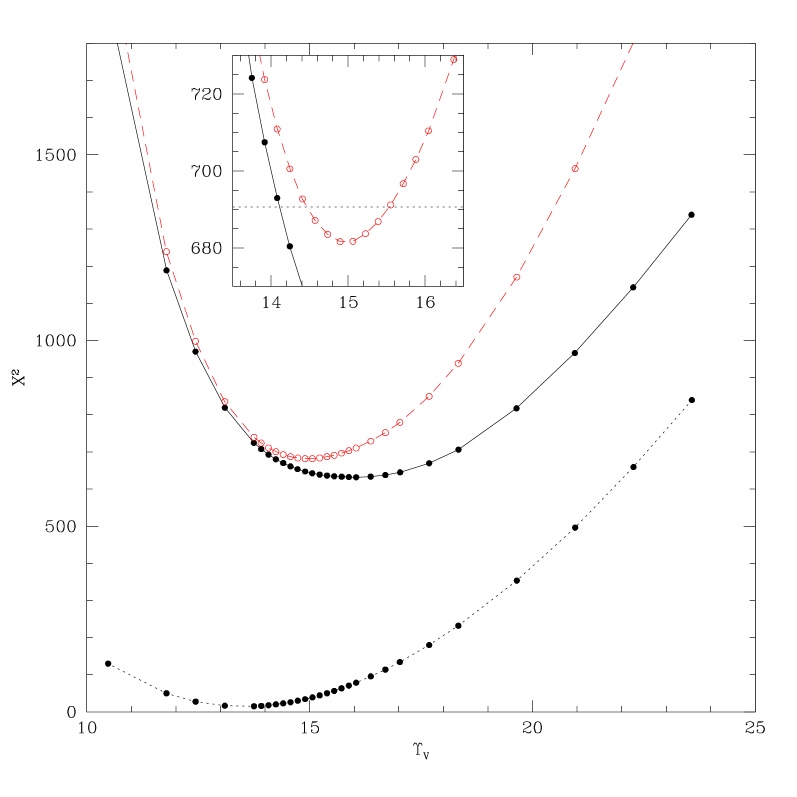
Figure 7: $\chi^{2}$ distributions for the models with spatially constant $\Upsilon_{V}$. The dotted line is $\chi^{2}_{\rm gas}$, the full line is $\chi^{2}_{\rm stars}$ and the dashed line (with open dots) corresponds to the combination of both type of constraints. The dots represent the actual model calculations. The inset shows in more details the region near the (combined) $\chi^{2}$ minimum. The horizontal dotted line has $\chi^{2}=\chi^{2}_{\rm min}+9$.

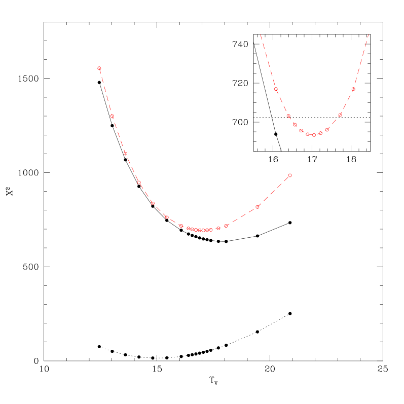
Figure 8: Same as Figure 7, but for the model with the logarithmic potential.

For an acceptable fit, one expects $\chi^{2}$ to be roughly equal to the number of data points ${\rm N_{data}}$ minus the number of degrees of freedom ${\rm N_{DOF}}$, which is not the case in the stellar fits because the statistical error bars do not reflect all uncertainties (see Section 2.2 and Figure 6). We show in Appendix A that the effective ${\rm N_{DOF}}$ is much smaller that ${\rm N_{data}}$. Following Kochanek (1994), we rescale the $\chi^{2}_{\rm stars}$ distribution such that $\chi^{2}_{\rm stars,\,min}=632$. Similarly, we consider the 15 gas data points with $|x^{\prime}|>3^{\prime\prime}$ for which the gas rotation curve is roughly flat and rescale the $\chi^{2}_{\rm gas}$ distribution, so that $\chi^{2}_{\rm gas,\,min}=15$. In Figure 7, we plot $\chi^{2}_{\rm gas}$, $\chi^{2}_{\rm stars}$, and the combined $\chi^{2}_{\rm comb}$ distribution as function of $\Upsilon_{V}$ for the models in which the mass follows the light. The minimum $\chi^{2}_{\rm min,\,comb}$ is attained for $\Upsilon_{V}=15.0\pm 0.6$, where the error bar corresponds to the formal 99.73 % confidence level or $3\,\sigma$ interval (i.e., the range of $\Upsilon_{V}$ for which $\chi^{2}_{\rm comb}=\chi^{2}_{\rm min}+9$). We perform the same exercise for the model with the logarithmic potential. In that case, $\Upsilon_{V}$ is defined as the mass enclosed within $15^{\prime\prime}$ divided by the total amount of light in the same volume, and we find $\Upsilon_{V}=17.0\pm 0.7$ at the same confidence level (Figure 8).

In order to compare with the sample of 37 bright ellipticals studied by van der Marel (1991), we first calculate the total absolute magnitude of NGC 2320 in B using his choice for $H_{0}$, and find ${\rm M_{B}}=-23\;h_{50}$. We then translate our value of $\Upsilon_{V}=15$ in the V–band into the R–band to place NGC 2320 on van der Marel’s Figure 6 (upper left panel). Using V–R of 0.77 (typical for K0 giants) we find $\Upsilon_{R}=8.0$. This value is 1.8 times higher than the prediction of his least–square fit relation at that absolute magnitude, making NGC 2320 a slight outlier. We have used data from larger radii than in van der Marel’s analysis and this could account for some of the discrepancy. Furthermore radially anisotropic models like ours tend to yield higher mass–to–light ratio than isotropic models (see Figure 6 of van der Marel & Franx, 1993); however, this would decrease $\Upsilon_{R}$ by only $\sim 20\%$ for NGC 2320.

4.3 Intrinsic velocity dispersions

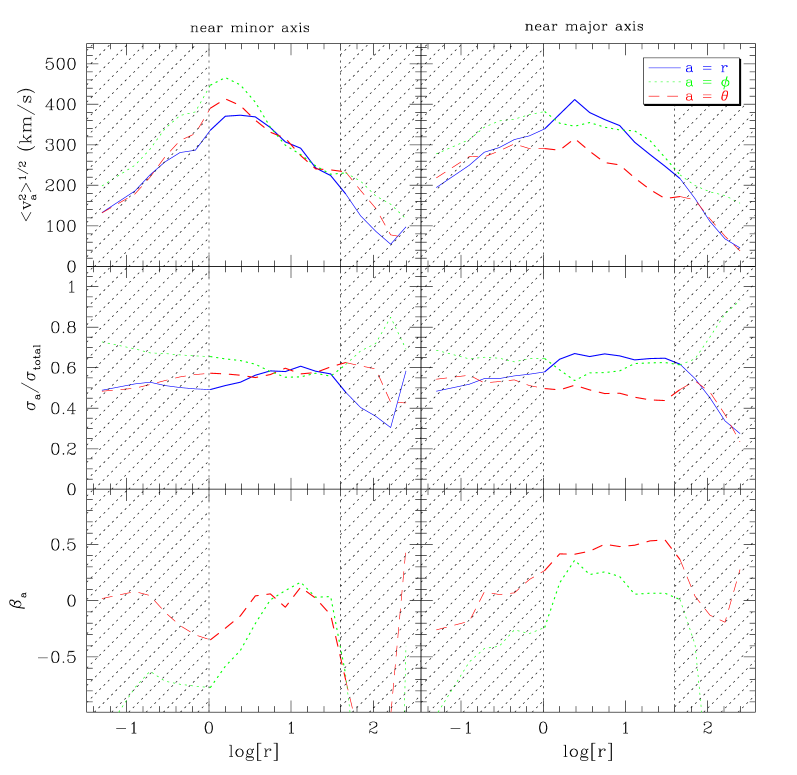
Figure 9: Anisotropy profiles of the model with $\Upsilon_{V}$ = 15. The first column is an average around the symmetry axis, and the second one around the equatorial plane. The first row shows the second moments in km/s, the second one the ratio of the dispersions to the total dispersion, and the last one shows the anisotropy parameter defined as $\beta_{a}=1-\sigma_{a}^{2}/\sigma_{r}^{2}$. The inset in the upper right panel explains the line convention.

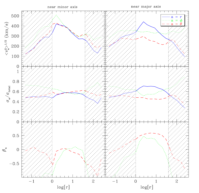
Figure 10: Same as Figure 9, but for the model with the logarithmic potential.

Using solutions with a statistically indistinguishable regularization (as defined in Section 5.5 of CvdB99), we compute second moments $\langle v_{R}^{2}\rangle^{1/2},\langle v_{\phi}^{2}\rangle^{1/2},\langle v_{\theta}^{2}\rangle^{1/2}$, ratio of dispersion profiles $\sigma_{R},\sigma_{\phi},\sigma_{\theta}$, and the anisotropy parameter $\beta$ (see e.g., Binney & Tremaine, 1987) along the major and minor axis for the best fit models. In Figure 9 we show these quantities for the best fit MGE model with $\Upsilon_{V}$ of 15. At a given radius the results are averaged over cells with different polar angles $\theta$: in the meridional plane, the first three angular sectors closest to the minor axis are averaged together (left column of Figure 9), as well as the remaining four closest to the major axis (right column). The first row displays the second moments as a function of radius. These moments are normalized by the total dispersion in the second row. In the last row, we plot the anisotropy parameter $\beta_{a}=1-\sigma_{a}^{2}/\sigma_{r}^{2}$ for $a=\phi$ (dotted line) or $a=\theta$ (dashed line). Positive $\beta$ corresponds to radial anisotropy. Figure 10 shows the same, but for the model with the logarithmic potential. For NGC 2320 the anisotropy exhibits similar general behavior for both types of models: they are dominated by radial anisotropy for most radii constrained by the data (between the shaded areas in Figures 9 and 10). On the major axis, $\beta_{\theta}\simeq 0.4-0.5$ and $\beta_{\phi}\simeq 0.0-0.3$, whereas $\beta_{\theta}\sim\beta_{\phi}\sim 0.0$ on the polar axis (except in the central $3^{\prime\prime}$).

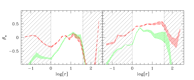
Figure 11: The anisotropy parameter as in Figure 9: the densely shaded region indicates the values of $\beta$ for models which lie in the formal 99.73 % confidence level region around the best fitting model (see Figure 7).

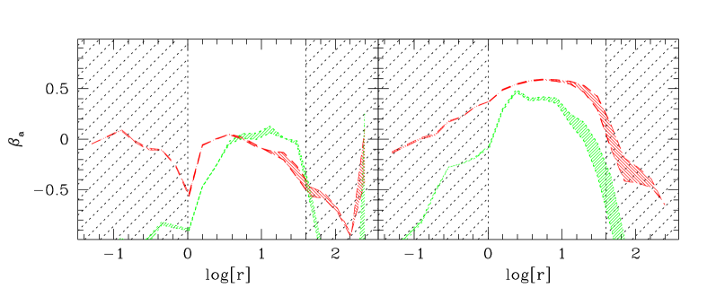
Figure 12: Same as Figure 11, but for the logarithmic potential mass model.

In Figure 11 and 12, we concentrate on the anisotropy parameter, $\beta$, to explore how much it varies among different statistically acceptable models. We compute the $\beta$–profiles of the two models that correspond to the 99.73 % confidence limit and shade the region in between them (Figure 11 and Figure 12), effectively estimating an error bar for $\beta$. All models in the 99.73 % confidence interval follow the same trend: they are radially anisotropic on the major axis and more nearly isotropic on the minor axis.

5 Conclusions and Discussion

We have constrained the orbital anisotropy of the stars in NGC 2320 by combining stellar VPs along multiple position angles with the kinematics of the ionized emission line gas. The nearly two–dimensional coverage of the galaxy by many long slit spectra tightly constrains the stellar dynamical model, while the gas kinematics provides constraint on the normalization of the gravitational potential, independent of stellar anisotropy issues.

The dynamical models are constructed following our extension of Schwarzschild’s orbit superposition technique described in C99. The best fitting model is dominated by radial anisotropy near the equatorial plane and is more isotropic on the polar axis. This conclusion is valid both for models in which the mass is proportional to the light and for models with a flat rotation curve at large radii (logarithmic potential). We find a best fit $\Upsilon_{V}$ of $15.0\pm 0.6$ for the radially constant $\Upsilon_{V}$ model and $\Upsilon_{V}(<15^{\prime\prime})=17.0\pm 0.7$ for the logarithmic one. We study the dispersion profiles of models for these intervals of $\Upsilon_{V}$ in order to determine the range of anisotropy among models that all fit the data. This range is small in general and all models in the $\Upsilon_{V}$ interval follow the same trend (i.e., radial anisotropy in the equatorial plane, isotropy near the symmetry axis). Radial anisotropy of the stellar objects has also been inferred from the modelling of some other objects (NGC 2434, NGC 1600, NGC 6703, NGC 1399, NGC 3377, NGC 3379, NGC 4473, NGC 5845 and M87).

It seems worth comparing to the dynamical structure of merger remnants produced by N–body simulations. Many merger simulations leading to the formation of an elliptical galaxy have concentrated on mergers of a pair of disk galaxies (Barnes 1992; Barnes & Hernquist 1996), of several disk galaxies (Barnes 1989; Weil & Hernquist 1996) or of small virialized clusters of spherical galaxies (Funato, Makino & Ebisuzaki 1993; Garijo, Athanassoula & Garcia–Gomez 1997). Dubinski (1998) carried out simulations embedded in a cosmological context and found that the anisotropy of the brightest cluster galaxy grows gently from $\beta=0.0$ near the center to $\beta=0.5$ at 3 $\rm R_{eff}$. Inside one $\rm R_{eff}$, his N–body model is mildly radially anisotropic ($\beta<0.3$). This is qualitatively consistent with our results for NGC 2320.

A comparison of NGC 2320 with Barnes’ results is more complicated: In his collisionless simulations, Barnes (1992) typically finds triaxial merger remnants with a large fraction of box orbits (see e.g., his figure 20). These box orbits do not exist in the axisymmetric case where only tube orbits are present. Therefore our axisymmetric models have no other choice than to put a lot of weight on low $L_{z}$ tubes to produce radial anisotropy. This is not the case for Barnes’ models: the box orbits (with $L_{z}=0$) are responsible for the radial anisotropy whereas his population of tube orbits seems fairly uniform in $L_{z}$ (see his Figures 20b, 21b and 22b).

Black holes, steep central density cusps and central gas concentrations can efficiently scatter stars on box orbits and destroy the triaxiality (see e.g., Gerhard & Binney 1985; Barnes & Hernquist 1996; Merritt & Quinlan 1998). In this scenario, the galaxy shape evolves towards axisymmetry, and its DF becomes closer to a $f(E,L_{z})$–form (Merritt 1999). Therefore, our anisotropic results for NGC 2320 argue against a scenario in which large amounts of gas flowed to the center during its formation. It would be interesting to investigate the existence of a central black hole and of a steep stellar cusp in NGC 2320, using higher resolution observations.

Appendix A Estimation of the number of degrees of freedom

For a good $\chi^{2}$ fit, one expects on average $\chi^{2}$ to be equal to $\chi^{2}_{\rm expected}={\rm N_{data}-N_{DOF}}$, where ${\rm N_{data}}$ is the number of data points and ${\rm N_{DOF}}$ is the number of degrees of freedom, if the errors are properly estimated and normally distributed. In our Schwarzschild models, we have many more weights that can be adjusted than we have data constraints. Yet, the projected properties of our orbits are not linearly independent and we have additional non–negativity, self–consistency and symmetry constraints; hence ${\rm N_{DOF}}$ is considerably smaller than the number of orbits. The key question is therefore how to determine the effective $\rm N_{DOF}$ for our orbit models ?

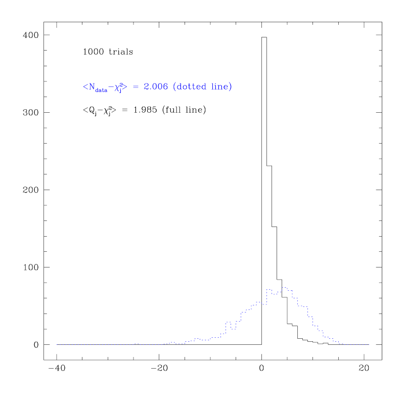
Figure 13: Histograms showing the broad distribution ${\rm N_{\rm data}-\chi^{2}_{j}}$ (dotted line) and the narrower distribution $Q_{j}-\chi^{2}_{j}$ (full line) for 1000 Monte–Carlo realizations. The effective $\rm N_{DOF}$ is the mean of these distributions. Here we show the case of a straight line, i.e., $\rm N_{DOF}=2$.

One can estimate $\rm N_{DOF}$ as $\langle{\rm N_{\rm data}}-\chi^{2}_{j}\rangle$, where this average is done over many Monte–Carlo realizations of the data and where $\chi^{2}_{j}$ of the $j$-realization is defined as $\sum_{i}^{\rm N_{data}}(y_{i}-y_{i,{\rm best-fit}})^{2}/\sigma_{i}^{2}$. Each of these realizations is generated according to a Gaussian distribution around each data point, with a variance equal to the corresponding error bar. The distribution ${\rm N_{data}}-\chi^{2}_{j}$ is broad, so its mean is not accurately defined for a modest number of realizations. Therefore we prefer to estimate $\rm N_{DOF}$ as the mean $\langle Q_{j}-\chi^{2}_{j}\rangle$, where $Q_{j}=\sum_{i}^{\rm N_{data}}(y_{i}-y_{i,{\rm true}})^{2}/\sigma_{i}^{2}$ for the $j^{th}$-realization. The $y_{i,{\rm true}}$ are the true underlying data points. In Figure 13, we illustrate the estimation of $\rm N_{DOF}$ with 20 fake data points drawn from and then fitted to a straight line function, i.e. $\rm N_{DOF}$=2. We generate 1000 data sets and show that the ${\rm N_{\rm data}}-\chi^{2}_{j}$ distribution is broader than $Q_{j}-\chi^{2}_{j}$.

We can apply the same procedure to the more complex case of our orbit model for NGC 2320. In the presence of the systematic deviations in the NGC 2320 data, we took the best–fitting model to the observational data as the true underlying distibution and generated 10 Monte–Carlo data sets normally distributed around it (according to the observed error bars). For each of these models, we performed a NNLS fit and computed $\langle Q_{j}-\chi^{2}_{j}\rangle$. We found $\rm N_{DOF}\simeq 25$, much smaller than ${\rm N_{\rm data}}$, which is 632 in this case. Therefore we have about 25 times more data constraints than effective degrees of freedom, implying a well–posed fitting problem.

References

Barnes, J. E. 1989, Nature, 338, 123

Barnes, J. E. 1992, ApJ, 393, 484

Barnes, J. E., & Hernquist, L. 1996, ApJ, 471, 115

Binney, J. J., & Tremaine S. D. 1987, Galactic Dynamics (Princeton: Princeton University Press)

Carollo, C. M., de Zeeuw, P. T., van der Marel, R. P., Danziger, I. J., & Qian, E. E. 1995, ApJ, 441, L25

Cinzano, P., van der Marel, R. P. 1994, MNRAS, 270, 325

Cretton, N., de Zeeuw, P. T., van der Marel, R. P., & Rix, H.-W. 1999, ApJS, 124, 383 (C99)

Cretton, N. & van den Bosch, F. C. 1999, ApJ, 514, 704 (CvdB99)

Dejonghe, H., de Bruyne, V., Vauterin, P., Zeilinger, W. W. 1996, A&A, 306, 363

Dejonghe, H. 1987, MNRAS, 224, 13

Dubinski, J. 1998, ApJ, 502, 141

Emsellem, E., Monnet, G., & Bacon, R. 1994, A&A, 285, 723

Funato, Y., Makino, J., & Ebisuzaki, T. 1993, PASJ, 45, 289

Garijo, A., Athanassoula, E., & Garcia–Gomez, C. 1997, A&A, 327, 930

Gebhardt, K., et al., 2000, AJ, in press (astro–ph/9912026)

Gerhard, O. E., Binney, J. J. 1985, MNRAS, 216, 467

Gerhard, O. E. 1993, MNRAS, 265, 213

Gerhard, O. E., Jeske, G., Saglia, R. P., Bender, R. 1998, MNRAS, 295, 197

Kochanek, C. S. 1994, ApJ, 436, 56

Lawson, C. L., & Hanson, R. J. 1974, Solving Least Squares Problems (Englewood Cliffs, New Jersey: Prentice–Hall)

Matthias, M., & Gerhard, O. E. 1999, MNRAS, 310, 879

Merritt, D. 1993, ApJ, 413, 79

Merritt, D., & Oh, S. P. 1997, AJ, 113, 1279

Merritt, D., & Quinlan, G. D. 1998, ApJ , 498, 625

Merritt, D. 1999, Comments on Modern Physics, Vol. 1, 39

Navarro, J., Frenk, C., & White, S. D. M. 1996, ApJ, 462, 563

Neistein, E., Maoz, D., Rix, H.-W., Tonry, J. L. 1999, AJ, 117, 2666

Prugniel, Ph., Heraudeau, Ph. 1998, AAS, 128, 299

Press, W. H., Teukolsky, S. A., Vetterling, W. T., & Flannery, B. P. 1992, Numerical Recipes (Cambridge: Cambridge University Press)

Richstone, D. O, et al. 1997, in The Nature of Elliptical Galaxies, Proceedings of the Second Stromlo Symposium, eds. Arnaboldi, M., da Costa, G., & Saha, P., p. 123

Rix, H.–W., & White, S. D. M. 1992, MNRAS, 254, 389

Rix, H.–W., Kennicutt, R. C., Braun, R., Walterbos, R. A. M. 1995, ApJ, 438, 155

Rix, H.-W., de Zeeuw, P. T., Cretton, N., van der Marel, R. P., & Carollo, C. M. 1997, ApJ, 488, 702

Saglia, R. P., Kronawitter, A., Gerhard, O. E., Bender, R. 1999, MNRAS, submitted, (astro–ph/9909446)

Statler, T. S., Smecker–Hane, T., Cecil, G. N. 1996, AJ, 111, 1512

Statler, T. S., Dejonghe, H., Smecker–Hane, T. 1999, AJ, 117, 126

van den Bosch, F. C., & Emsellem E. 1998, MNRAS, 298, 267

van der Marel, R. P. 1991, MNRAS, 253, 710

van der Marel, R. P., & Franx, M. 1993, ApJ, 407, 525

van der Marel, R. P., Cretton, N., de Zeeuw, P. T., & Rix, H. W. 1998, ApJ, 493, 613

Weil, M., Hernquist, L. 1996, ApJ, 460, 101

Figure 2: Mean line–of–sight velocity and dispersion of the gas along the major axis (MMT spectra). The central velocity gradient is affected by the wide slit ($3.5^{\prime\prime}$).

Figure 6: Kinematic data for all the slits and fits of the two best fit models: the full line is the model where the mass follows the light and the dotted line is the model with the logarithmic potential. The columns have been organized in increasing Position Angle order, starting from the MMT major axis. The top line shows the fit of the (normalized) mass constraints in the meridional plane and in the plane of the sky. In the fit of the meridional plane constraints, we exclude the cells closest to the symmetry axis. This explains the jagged appearance of the fit for these constraints.

Table 1: Summary of the kinematic observations.

$j$	name	telescope	slit width	date	radial extent	# of points	S/N
(1)	(2)	(3)	(4)	(5)	(6)	(7)	(8)
1	MMT-140	MMT	3.5	17 Feb 1996	37	23	25
2	MMT-50	MMT	3.5	17 Feb 1996	23	12	25
3	050	KPNO 4m	2.5	2 Mar 1998	17	8	12
4	100	KPNO 4m	2.5	27 Feb 1998	18	10	10
5	130	KPNO 4m	2.5	27 Feb 1998	27	11	12
6	142	KPNO 4m	2.5	2 Mar 1998	24	12	12
7	175	KPNO 4m	2.5	27 Feb 1998	19	10	10
8	b000	KPNO 4m	2.5	1 Mar 1998	24	9	15
9	b020	KPNO 4m	2.5	1 Mar 1998	27	10	15
10	b100	KPNO 4m	2.5	27 Feb 1998	45	18	10
11	b130	KPNO 4m	2.5	27 Feb 1998	44	19	10
12	b175	KPNO 4m	2.5	27 Feb 1998	43	16	10

Note. — Column (1) gives the number of the spectrum; column (2) its name (chosen after its position angle); column (3) the telescope where it was taken; column (4) the slit width (in arcseconds); column (5) the date of observation; column (6) the maximum radial extension (in arcseconds); column (7) the number of data points (after pixel binning) for the stellar data; column (8) the S/N for the stellar data.

Table 2: Parameters of MGE model for the luminous density profile.

$j$	$I_{j}$	$a_{j}$	$q_{j}$
(1)	(2)	(3)	(4)
1	287764585.49	0.820	0.544
2	18868477.1	3.000	0.443
3	1826940.9	8.585	0.419
4	219268.2	19.061	0.505
5	9359.8	56.370	0.676

Note. — Column (1) gives the index number of each Gaussian. Column (2) gives its central luminosity density (in ${\rm\,L_{\odot}}/{\rm arcsec}^{3}$); column (3) its standard deviation (which expresses the size of the Gaussian along the major axis) and column (4) its flattening. All Gaussians have the same position angle and the same center.