METRIC PERTURBATIONS AND INFLATIONARY PHASE TRANSITIONS

Abstract

We study the out of equilibrium dynamics of inflationary phase transitions and compute the resulting spectrum of metric perturbations relevant to observation. We show that simple single field models of inflation may produce an adiabatic perturbation spectrum with a blue spectral tilt and that the precise spectrum depends on initial conditions at the outset of inflation.

1 Field Evolution

We work in a spatially flat Friedmann-Robertson-Walker universe with scale factor $a(t)$ and take the inflaton to be a real scalar field with Lagrangian

$$L=\frac{1}{2}\nabla^{\mu}\Phi\nabla_{\mu}\Phi-\left[\frac{3\mu^{4}}{2\lambda}-\frac{1}{2}\mu^{2}\Phi^{2}+\frac{\lambda}{4!}\Phi^{4}\right]\;.$$ (1)

We break up the field $\Phi$ into its expectation value, defined within the closed time path formalism, [1] and fluctuations about that value:

$$\Phi(\vec{x},t)=\phi(t)+\psi(\vec{x},t)\;,\;\;\phi(t)\equiv\langle\Phi(\vec{x},t)\rangle\;.$$

By imposing a Hartree resummation, [2] we arrive at the following equations of motion for the inflaton: [3]

$$\ddot{\phi}+3\frac{\dot{a}}{a}\dot{\phi}-\mu^{2}\phi+\frac{\lambda}{6}\phi^{3}+\frac{\lambda}{2}\langle\psi^{2}\rangle\phi=0\;,$$ (2)

$$\left[\frac{d^{2}}{dt^{2}}+3\frac{\dot{a}}{a}\frac{d}{dt}+\frac{k^{2}}{a^{2}}-\mu^{2}+\frac{\lambda}{2}\langle\psi^{2}\rangle+\frac{\lambda}{2}\phi^{2}\right]f_{k}=0\;.$$ (3)

The fluctuation $\langle\psi^{2}\rangle$ is determined from the mode functions $f_{k}$:

$$\langle\psi^{2}\rangle=\int\frac{d^{3}k}{(2\pi)^{3}}|f_{k}|^{2}\;.$$ (4)

For $a(t_{0})=1$, the initial conditions on the mode functions are

$$f_{k}(t_{0})=\frac{1}{\sqrt{2\omega_{k}}}\;,\;\;\dot{f}_{k}(t_{0})=\left(-\dot{a}(t_{0})-i\omega_{k}\right)f_{k}(t_{0})\;,$$ (5)

with

$$\omega_{k}^{2}\equiv k^{2}-\mu^{2}+\frac{\lambda}{2}\langle\psi^{2}\rangle+\frac{\lambda}{2}\phi^{2}-\frac{R(t_{0})}{6}\;.$$

$R(t_{0})$ is the initial Ricci scalar. For small $k$, we modify $\omega_{k}$ either by means of a quench or by explicit deformation so that the frequecies are real. [4, 5]

The gravitational dynamics are determined by the semi-classical Einstein equation. [6] For a minimally coupled inflaton we have

$$\frac{\dot{a}^{2}}{a^{2}} = \frac{8\pi G_{N}}{3}\left[\frac{1}{2}\dot{\phi}^{2}+\frac{1}{2}\langle\dot{\psi}^{2}\rangle+\frac{1}{2a^{2}}\left\langle(\vec{\nabla}\psi)^{2}\right\rangle\right.$$ (6)

$$+ \left.\frac{3\mu^{4}}{2\lambda}-\frac{1}{2}\mu^{2}\left(\phi^{2}+\langle\psi^{2}\rangle\right)+\frac{\lambda}{24}\left(\phi^{4}+3\langle\psi^{2}\rangle^{2}+6\phi^{2}\langle\psi^{2}\rangle\right)\right]\;,$$

where $G_{N}$ is Newton’s gravitational constant, and

$$\langle\dot{\psi}^{2}(t)\rangle \equiv \int\frac{d^{3}k}{(2\pi)^{3}}|\dot{f}_{k}|^{2}\;,$$ (7)

$$\left\langle\left(\vec{\nabla}\psi(t)\right)^{2}\right\rangle \equiv \int\frac{d^{3}k}{(2\pi)^{3}}k^{2}|f_{k}|^{2}\;.$$ (8)

Each of these integrals is regulated using a cutoff with the divergences absorbed into a renormalization of the parameters of the theory. [4]

A typical field evolution is depicted in Fig. 1.

2 Metric Perturbations

Following the procedure of Mukhanov, Feldman and Brandenberger, [7] we arrive at the expression for the density contrast at mode re-entry:[8]

$$|\delta_{h}(k)| = \sqrt{\frac{2}{75\pi}}\frac{1}{M_{Pl}\left(\dot{\phi}^{2}+\langle\dot{\psi}^{2}\rangle\right)}\left[\frac{3\mu^{4}}{2\lambda}-\frac{1}{2}\mu^{2}\left(\phi^{2}+\langle\psi^{2}\rangle\right)\right.$$ (9)

$$\left.+\frac{\lambda}{24}\left(\phi^{4}+6\phi^{2}\langle\psi^{2}\rangle+3\langle\psi^{2}\rangle^{2}\right)\right]^{1/2}$$

$$\times \left[\mu^{4}\left(\phi^{2}+\langle\psi^{2}\rangle\right)-\frac{\lambda\mu^{2}}{3}\left(\phi^{4}+6\phi^{2}\langle\psi^{2}\rangle+3\langle\psi^{2}\rangle^{2}\right)\right.$$

$$\left.+\frac{\lambda^{2}}{36}\left(\phi^{6}+15\phi^{4}\langle\psi^{2}\rangle+45\phi^{2}\langle\psi^{2}\rangle^{2}+15\langle\psi^{2}\rangle^{3}\right)\right]^{1/2}\;.$$

The computation of the tilt parameter $n_{s}-1$ is straightforward, given (9):

$$n_{s}-1\equiv\left.\frac{d(\ln|\delta_{h}(k)|)}{d\ln(k)}\right|_{k=aH}\;.$$ (10)

As gravitational wave perturbations do not directly interact with the inflaton field, they may be related directly to the expansion rate. The amplitude of gravitational waves is simply: [7]

$$|\delta_{g}(k)|=\frac{2}{\sqrt{3\pi}}\frac{H}{M_{Pl}}\;,$$ (11)

All expressions are to be evaluated when the given scale $k$ first crosses the horizon, $k=aH$.

An example perturbation spectrum is shown in Fig. 2, while Fig. 3 shows the dependence of the spectrum on the initial state for a number of possible evolutions. Both of these figures show distinct regions characterized by a blue spectral tilt.

References

Figure 1: The mean field $\phi(t)/f$, the fluctuation $<\psi^{2}(t)>^{1/2}/f$, and the Hubble parameter $H(t)/\mu$ vs. $t$ with $\phi(t_{0})=0.4H_{0}/2\pi$, $\dot{\phi}(t_{0})=0$, $H_{0}=2\mu$, $\lambda/8\pi^{2}=10^{-16}$, and $f\equiv\mu\sqrt{6/\lambda}$.

Figure 2: The scalar amplitude $\delta_{h}$, the scalar tilt $n_{s}-1$, and the tensor amplitude $\delta_{g}$ as a function of the number of $e$-folds $N$ before the end of inflation that the scale first crosses the horizon. Parameters are as in Fig. 1.

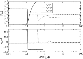
Figure 3: The scalar amplitude $\delta_{60}$ and tilt $n_{60}-1$ of the scale crossing the horizon $60$ $e$-folds before the inflation ends vs. $2\pi\phi(t_{0})/\mu$ with $\dot{\phi}(t_{0})=0$, $\lambda/8\pi^{2}=10^{-16}$ and several values of $H_{0}$.

References

[1] J. Schwinger, J. Math. Phys.2, 407 (1961);
L. V. Keldysh, Sov. Phys. JETP20, 1018 (1965).
[2] See, for example, A.L. Fetter and J.D. Walecka,
Quantum Theory of Many-Particle Systems, McGraw-Hill, New York (1971).
[3] D. Cormier, Non-Equilibrium Field Theory Dynamics
in Inflationary Cosmology, hep-ph/9804449 (1998).
[4] D. Boyanovsky, D. Cormier, H.J. de Vega, R. Holman and P. Kumar
Phys. Rev. D57, 2166 (1998).
[5] D. Boyanovsky, D. Cormier, H.J. de Vega and R. Holman,
Phys. Rev. D55, 3373 (1997).
[6] N.D. Birrell and P.C.W. Davies, Quantum
Fields in Curved Space, Cambridge Univ. Press, Cambridge, (1986).
[8] D. Cormier and R. Holman, Spinodal Decomposition
and Inflation: Dynamics and Metric Perturbations, hep-ph/9912483 (1999).