A multipole-Taylor expansion for the potential
of gravitational lens MG J0414+0534

Abstract

We employ a multipole-Taylor expansion to investigate how tightly the gravitational potential of the quadruple-image lens MG J0414+0534 is constrained by recent VLBI observations. These observations revealed that each of the four images of the background radio source contains four distinct components, thereby providing more numerous and more precise constraints on the lens potential than were previously available. We expand the two-dimensional lens potential using multipoles for the angular coordinate and a modified Taylor series for the radial coordinate. After discussing the physical significance of each term, we compute models of MG J0414+0534 using only VLBI positions as constraints. The best-fit model has both interior and exterior quadrupole moments as well as exterior $m=3$ and $m=4$ multipole moments. The deflector centroid in the models matches the optical galaxy position, and the quadrupoles are aligned with the optical isophotes. The radial distribution of mass could not be well constrained. We discuss the implications of these models for the deflector mass distribution and for the predicted time delays between lensed components.

1 Introduction

There are now about 40 observed examples of “strong” gravitational lensing, in which multiple images of a background object are produced by the gravitational potential of an intervening object (Kochanek et al. (1999)). Constructing models for the gravitational potential of the deflecting mass in these systems is of fundamental importance, in the first place to verify that the observed system is truly a gravitational lens. A crucial hurdle for every promising gravitational lens candidate is to have its image configuration reproduced, at least approximately, by a plausible model for the deflecting mass distribution. If this cannot be achieved, the lensing interpretation must be seriously doubted.

Once this and other tests for lensing are passed successfully, however, model construction moves beyond a plausibility check into a direct measurement of the mass distribution of the lens. Lensing makes a unique contribution because it is sensitive to all forms of mass (including dark matter), yet does not depend on any luminous tracers in the lens. Lens modeling is also a crucial step in the enterprise of determining cosmological parameters by measuring the time delays between the light curves of multiple images. A successful model will predict the values of these time delays in terms of parameters such as $H_{0}$, $\Omega_{m}$, and $\Omega_{\Lambda}$. These parameters can then be constrained by the time-delay measurements (Refsdal 1964, (1966); for recent examples see Haarsma et al. (1999), Lovell et al. (1998)). The appeal of this technique is that it does not make use of the usual chain of intermediate distance indicators and their associated uncertainties.

The determinations of mass distributions and cosmological parameters are both frustrated by the main challenge of lens modeling: it is a poorly-constrained inverse problem with unknown systematic errors. It is neither obvious which parameterized model for the gravitational potential should be chosen, nor how precisely the parameters are constrained by the data. The choice of parameterization for the gravitational potential is usually dictated by two factors: preconceptions about the mass distribution of galaxies (based on the distribution of luminous matter and/or velocity dispersions), and ease of computation. Some examples are singular isothermal spheres, elliptical density profiles, elliptical potential contours, and triaxial density profiles (see e.g. Schneider & Weiss (1991); Nair & Garrett (1997); Chae, Khersonksy & Turnshek (1998)). Added to these are terms representing external “shear” from the tidal forces of neighboring mass concentrations. Such models have all been used successfully to reproduce the image configurations of the known sample of lenses, at least qualitatively, which leads one to wonder how well the observations of strong lensing actually constrain the lens potential.

Kochanek (1991) was the first to investigate this question systematically. He attempted to model each of 12 different lenses using a set of 6 different parameterized potentials. The potentials he considered were point masses and singular isothermal spheres, added to shear terms with one of three radial dependencies. He found that the total mass in the region between the multiple images is well constrained, but the radial dependence of the potential is not. This was because the multiple images are typically located close to the “Einstein ring” of the lens, so the constraints on the potential are correspondingly limited to a small range in radius. Kochanek suggested (but did not carry out) a Taylor expansion, parameterized by the deviation from the ring radius, as a way to turn this fact to advantage.

The purpose of this paper is to elaborate upon this suggestion and apply it to a particular quadruple-image gravitational lens, MG J0414+0534. We expand the potential as a series of multipoles in angle, and as a modified Taylor series in radius. The resulting series has three advantages over traditional lens models. One, it is mathematically general, and therefore less subject to preconceptions about the galactic mass distribution (which, after all, is what is trying to be determined). Two, the degeneracies in the lens equation and the moments of the mass distribution have simple correspondences to individual terms of the series. Three, each successive term in the series is expected to contribute a smaller amount to the light deflection, so long as the radial parameter is small and the angular dependence of the potential is smooth. This allows the complexity of the model to be easily prescribed by the truncation of the series. However, although the first assumption (the smallness of the radial parameter) is empirically true for quadruple-image lenses, the second assumption (the angular smoothness of the potential) is open to question. Nevertheless, in the face of our ignorance of true galaxy structure, we employ a multipole expansion because of its simplicity and generality.

The disadvantage of a mathematically general expansion (rather than one that is motivated by astrophysical preconceptions) is that the number of parameters is large. In many cases, especially for the double-image lenses, the number of parameters would be comparable to or more than the number of observational constraints. This is probably why such an expansion has not been used previously. However, recent VLBI images of MG J0414+0534 provide a much larger body of constraints than were previously available (Trotter (1998)). Each of the four lensed images was found to contain four components, with clear correspondences between the components of different images. This provides 16 components whose positions are known with milliarcsecond precision, thereby creating a testbed for the multipole-Taylor expansion.

This paper will be organized as follows. The next section describes prior optical and radio observations of MG J0414+0534, in addition to the latest VLBI map. Section 3 presents the formalism for our series expansion, discusses the physical significance of each term, and identifies the terms that cannot be constrained due to degeneracies in the lens equation. Some previous models for MG J0414+0534 are discussed and compared to our technique. Section 4 explains the numerical methods we employed and presents the best-fit results. Finally, section 5 discusses the implications of these results for the mass distribution of the lens and the time delays between images.

2 Observations of MG J0414+0534

The radio source MG J0414+0534 was first identified by Hewitt et al. (1992) as a gravitational lens during a systematic search for lenses in the MIT-Green Bank 5 GHz radio catalog. In both optical and radio images it has four components, which have been called A1, A2, B, and C, in order of decreasing brightness. The radio components all have spectral index $\alpha=-0.80\pm 0.02$ (Katz, Moore & Hewitt (1997)), and the optical components are all exceedingly red. However, the A1/A2 radio flux ratio ($\sim 1.1$) and optical flux ratio ($\sim 2.5$) do not agree, even though gravitational light deflection is independent of wavelength. The discrepancy could be caused by a number of factors (Angonin-Willaime et al. (1994)), including dust (McLeod et al. (1998)) and microlensing (Witt, Mao & Schechter (1995)).

Schechter & Moore (1993) discovered the lensing galaxy in the $I$ band, along with a faint object $1\arcsec$ west of component B which they named object X. The optical/infrared spectrum of the lensed source resembles a very reddened quasar at $z_{s}=2.639\pm 0.002$ (Lawrence et al. (1995)). The redshift of the lensing galaxy is $z_{l}=0.9584\pm 0.0002$ (Tonry & Kochanek (1998)). The best presently published optical photometry (uncertainty $\approx 0.004$ mag) and astrometry (uncertainty $\approx 0.02\arcsec$) for this system were obtained with Hubble Space Telescope (HST) WFPC2/PC1 observations by Falco, Lehár & Shapiro (1997), who also detected a blue arc extending from A1 to A2 to B.

The deepest radio observations to date did not detect a fifth radio component in the system (Katz, Moore & Hewitt (1997)). Higher-resolution radio maps, using MERLIN (Garrett et al. (1993)) and VLBI (Patnaik & Porcas (1996)), showed substructure within the four images of MG J0414+0534. In particular, the VLBI map resolved images A1, A2, and B into two components each, and revealed image C to be extended. Previous attempts to use VLBI constraints to perform lens modeling, however, were hampered by the low signal-to-noise ratio of the available data (Ellithorpe (1995)).

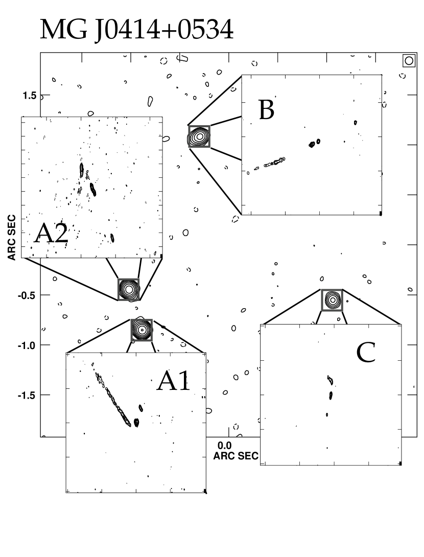
Figure 1: High-resolution maps of the four images of MG J0414+0534, observed at 5 GHz with the VLBA, are shown superimposed on the 22 GHz VLA map of Katz, Moore & Hewitt (1997) (kindly supplied by C. Katz).

As part of a 1995 study to test the feasibility of using the NRAO Very Long Baseline Array (VLBA) to monitor the time-variability of various radio-loud lenses, we obtained 5 GHz images of MG J0414+0534. These observations and the data reduction procedure are described in detail elsewhere (Trotter (1998)) and will be presented in a future paper; only the results are summarized here. The synthesized beam was $1.5\times 3.5$ milliarcseconds, and the RMS thermal noise was about 0.15 mJy/beam, close to the theoretical limit. The peak fluxes in the maps of each of the four images ranged from 21 to 110 mJy/beam, allowing a much higher signal-to-noise ratio than was previously available. Within each image were detected four components. The compact components p, q, and r were labeled in order of decreasing brightness; there is also one extended component, labeled s. The four maps are shown in Figure 1, superimposed on a lower-resolution VLA map. The sub-components are labeled in the larger maps shown in Figure 2. The locations, fluxes, and extents of the components were determined by least-squares fitting to a set of elliptical Gaussian parameters. Table 1 lists the locations and fluxes of the 16 VLBI components.

3 The modified multipole-Taylor expansion

The motivation behind our method for lens modeling is to expand the lens potential in a manner which preserves a measure of mathematical generality and in which the terms that can and cannot be constrained by lensing data are clearly separated. We have tried to arrange for the parameters in our expansion to be sensitive to what can be learned from lensing data, rather than what one would wish a priori to learn. In this section we will develop this expansion in detail, describe the physical significance and constrainability of each term, and compare our expansion to other commonly-used parameterizations.

3.1 The multipole-Taylor expansion

The goal of lens modeling is to deduce the two-dimensional gravitational lens potential, which is defined in a way similar to the definitions of Schneider, Ehlers & Falco (1992) and Narayan & Bartelmann (1996):

$$\Phi({\bf r})=\frac{2D_{LS}}{D_{L}D_{S}}\int{dz\ \Phi_{N}(D_{L}{\bf r},z)}.$$ (1)

Here ${\bf r}$ is the angular coordinate measured from an arbitrary optic axis, $z$ is the line-of-sight coordinate, and $\Phi_{N}$ is the Newtonian gravitational potential of the lens. The angular diameter distances $D_{L}$, $D_{S}$, and $D_{LS}$ are from observer to lens, observer to source, and lens to source, respectively. As elsewhere in this paper, the speed of light has been set to 1 by a choice of units.

The lens potential is related to the surface mass density of the lensing object by the two-dimensional Poisson equation,

$$\nabla_{{\bf r}}^{2}\Phi({\bf r})=8\pi G\frac{D_{L}D_{LS}}{D_{S}}\sigma({\bf r})=\frac{2\sigma({\bf r})}{{\sigma_{\rm c}}}.$$ (2)

Implicit in the above equation is the definition of the critical surface mass density, ${\sigma_{\rm c}}=(1/4\pi G)(D_{S}/D_{L}D_{LS})$. The lens potential determines the image configuration via the lens equation,

$${\bf s}={\bf r}-{\mbox{\boldmath{$\nabla$}}}_{{\bf r}}\Phi({\bf r}),$$ (3)

where ${\bf r}$ is the image position and ${\bf s}$ is the source position. The typical procedure in lens modeling is to adopt a parameterized form for $\Phi$, and then fix the parameters by minimizing an error function $\chi^{2}$. The error function may represent the deviations between the observed images and the images that are projected through the model potential from a model source distribution. Alternatively, the error function may represent the deviations between source positions that are back-projected from the various images (which is computationally simpler), as explained further in section 55.

The parameterization we adopt is a multipole-Taylor expansion. The first step is to expand the potential $\Phi({\bf r})$ in terms of a complete set of orthogonal basis functions which make the Poisson equation separable:

$$\Phi(r,\theta)=\Phi_{0}(r)+\sum_{m=1}^{\infty}{{\bf\Phi}}_{m}(r)\cdot({\hat{\bf x}}\cos m\theta+{\hat{\bf y}}\sin m\theta)$$ (4)

The function $\Phi_{0}(r)$ is the monopole, and the vector-like functions ${{\bf\Phi}}_{m}(r)$ are the higher multipoles. Schneider & Weiss (1991) also carried out a multipole expansion of the lens potential in this manner. The motivation for this expansion is that each multipole moment of the potential depends only on the corresponding multipole moment of the surface mass density. Specifically, the relations are (Kochanek (1991)):

$$\Phi_{0}(r) = {\rm constant}+2\ln r\int_{0}^{r}dr^{\prime}\,r^{\prime}\frac{\sigma_{0}(r^{\prime})}{{\sigma_{\rm c}}}+2\int_{r}^{\infty}dr^{\prime}\,r^{\prime}\ln r^{\prime}\frac{\sigma_{0}(r^{\prime})}{{\sigma_{\rm c}}}$$ (5)

$${{\bf\Phi}}_{m}(r) = -\frac{r^{-m}}{m}\int_{0}^{r}dr^{\prime}\,r^{\prime(1+m)}\frac{{\mbox{\boldmath$\sigma$}}_{m}(r^{\prime})}{{\sigma_{\rm c}}}-\frac{r^{m}}{m}\int_{r}^{\infty}dr^{\prime}\,r^{\prime(1-m)}\frac{{\mbox{\boldmath$\sigma$}}_{m}(r^{\prime})}{{\sigma_{\rm c}}}.$$ (6)

For smooth mass distributions, only the few lowest-order terms in the multipole expansion of the surface mass density are expected to be significant, and the rest may be neglected. By reference to equations 5 and 6 it is clear that this is equivalent to neglecting the higher multipole components of the potential. For modeling purposes, one may truncate the expansion of the potential at the desired level.

The radial dependence of $\Phi_{0}(r)$ and ${{\bf\Phi}}_{m}(r)$ must also be parameterized to be suitable for use in lens modeling. Lensed images constrain ${\mbox{\boldmath{$\nabla$}}}\Phi$ and $\partial_{i}\partial_{j}\Phi$ at the locations of the images. For Einstein rings and quadruple-image lenses (“quads”), the images are typically near the lens’s characteristic ring radius. Therefore, following the suggestion of Kochanek (1991), we expand the radial dependence of each multipole moment of the potential as a Taylor series in the parameter $\rho=(r-b)/b$, where $b$ is the Einstein ring radius. (The meaning of the Einstein ring radius for a non-circular lens is discussed below, in section 3.2.) This series should converge quickly for image positions located at $r\approx b$. For example, $|\rho|<0.2$ for all of the components in MG J0414+0534.

The resulting expansion of the lens potential is:

$$\frac{1}{b^{2}}\Phi(r,\theta) = {\rm const}+\rho+\frac{1}{2}\rho^{2}f_{2}+\sum_{t=3}^{\infty}\frac{1}{t!}\rho^{t}f_{t}$$

$$-\sum_{m=1}^{\infty}\left(\left\{{{{\bf M}}^{\rm sum}_{m}}+\rho m{{{\bf M}}^{\rm diff}_{m}}+\sum_{t=2}^{\infty}\frac{1}{t!}\rho^{t}{{\bf F}}_{mt}\right\}\cdot{({{{\hat{\bf x}}\cos m\theta+{\hat{\bf y}}\sin m\theta}})}\right),$$

parametrized by the origin of the expansion $(g_{x},g_{y})$, the ring radius $b$, the monopole parameters $f_{t}$, and the higher multipole parameters ${{{\bf M}}^{\rm sum}_{m}}$, ${{{\bf M}}^{\rm diff}_{m}}$, and ${{\bf F}}_{mt}$. We use $t$ as an integral index, contrary to convention, because of the mnemonic value of associating $t$ with Taylor and $m$ with multipole. The additive constant $f_{0}$ does not affect light deflection. Because we factor out the ring radius $b$, and then use it as a parameter, we have $f_{1}=1$. The $m\geq 1$ multipoles with $t=0$ and $t=1$ received the special names ${{{\bf M}}^{\rm sum}_{m}}$ and ${{{\bf M}}^{\rm diff}_{m}}$ for reasons that will become apparent in the next section. The model parameters $g_{x}$ and $g_{y}$, which specify the location of the origin of coordinates, are implicit in equation 3.1. To simplify the interpretation of the multipole moments, this origin should be centered on the deflector. In section 3.4 it will be shown how this condition may be enforced during the model-fitting procedure.

3.2 Physical significance of the expansion parameters

Although the potential $\Phi({\bf r})$ is the quantity most directly constrained by observations of lensing, it is the surface mass density $\sigma({\bf r})$ that is usually of direct astrophysical interest. In this section the correspondence between the the parameters in the multipole-Taylor expansion of $\Phi({\bf r})$ and the multipoles of $\sigma({\bf r})$ will be made explicit. This is useful because the multipole moments of the surface mass density have a simple physical meaning. This meaning will be reviewed first, then the correspondence between the multipole-Taylor parameters and the surface mass density multipoles will be given. When $\sigma({\bf r})$ is expanded in a multipole series as in equation 4, it can be shown that:

$$\sigma_{0}(r) = \frac{1}{2\pi}{\int_{0}^{2\pi}}d\theta\sigma(r,\theta)$$ (8)

$${\mbox{\boldmath$\sigma$}}_{m}(r) = \frac{1}{\pi}{\int_{0}^{2\pi}}d\theta\sigma(r,\theta){({{{\hat{\bf x}}\cos m\theta+{\hat{\bf y}}\sin m\theta}})}.$$ (9)

These expressions make the physical meaning of the multipoles clear. The monopole moment $\sigma_{0}(r)$ is the average surface mass density in an infinitesimally narrow annulus of radius $r$, or, equivalently, the angularly-averaged surface mass density. The multipoles ${\mbox{\boldmath$\sigma$}}_{m}(r)$ describe the distribution of matter around that annulus. In particular, the dipole moment ${\mbox{\boldmath$\sigma$}}_{1}(r)$ points to the center of mass ${\bf x}_{c}$ of the annulus, viz.,

$$\frac{{\bf x}_{c}}{r}=\frac{1}{2}\frac{{\mbox{\boldmath$\sigma$}}_{1}(r)}{\sigma_{0}(r)}.$$ (10)

Likewise, the quadrupole moment ${\mbox{\boldmath$\sigma$}}_{2}(r)$ arises from an elongated mass distribution. The ${\mbox{\boldmath$\sigma$}}_{3}(r)$ term arises from any triangularity in the mass distribution. Any quadrangularity, e.g. boxiness or diskiness, will give rise to a nonzero ${\mbox{\boldmath$\sigma$}}_{4}(r)$ term. The multipole ${\mbox{\boldmath$\sigma$}}_{m}(r)$ can also be expressed as a magnitude $|{\mbox{\boldmath$\sigma$}}_{m}(r)|$ and an angle ${\psi_{\sigma_{m}}}(r)$,

$${\mbox{\boldmath$\sigma$}}_{m}(r)=|{\mbox{\boldmath$\sigma$}}_{m}(r)|({\hat{\bf x}}\cos m{\psi_{\sigma_{m}}}(r)+{\hat{\bf y}}\sin m{\psi_{\sigma_{m}}}(r)),$$ (11)

rather than by its ${\hat{\bf x}}$ and ${\hat{\bf y}}$ components. Twisted isodensity contours cause a change in the angle ${\psi_{\sigma_{m}}}(r)$ with radius. In particular, a relative excess of mass at radius $r$ in any of the $m$ directions ${\psi_{\sigma_{m}}}(r)+2\pi n/m$ (where $n\leq m$ is a positive integer) will contribute to the multipole moment ${\mbox{\boldmath$\sigma$}}_{m}(r)$. It follows from the positivity of the surface mass density that $|{\mbox{\boldmath$\sigma$}}_{m}(r)|\leq 2\sigma_{0}(r)$. The multipole moment attains its maximum amplitude only if all the mass in the annulus at radius $r$ is clumped at the equally spaced angles ${\psi_{\sigma_{m}}}(r)+2\pi n/m$, though it need not be evenly divided between these angles. In this manner, knowledge of the mass density’s multipole moments gives a direct picture of the location of the mass.

We now relate the expansion parameters of the lens potential to the multipole moments of the surface mass density, by expanding equations 5 and 6 in a Taylor series about $r=b$. For the monopole,

$$f_{t}\equiv\left.{\frac{1}{b^{2}}{b^{t}\frac{d^{t}}{dr^{t}}}}\Phi_{0}(r)\right|_{r=b},$$ (12)

of which the first four terms are:

$$f_{0}\equiv{\frac{1}{b^{2}}}\Phi_{0}(b) = {\rm const}$$ (13)

$$f_{1}\equiv\left.{\frac{1}{b^{2}}{b\frac{d}{dr}}}\Phi_{0}(r)\right|_{r=b} = 1$$ (14)

$$f_{2}\equiv\left.{\frac{1}{b^{2}}{b^{2}\frac{d^{2}}{dr^{2}}}}\Phi_{0}(r)\right|_{r=b} = -1+\frac{2\sigma_{0}(b)}{{\sigma_{\rm c}}}$$ (15)

$$f_{3}\equiv\left.{\frac{1}{b^{2}}{b^{3}\frac{d^{3}}{dr^{3}}}}\Phi_{0}(r)\right|_{r=b} = 2-\frac{2\sigma_{0}(b)}{{\sigma_{\rm c}}}+2\left.{{b\frac{d}{dr}}}\left(\frac{\sigma_{0}(r)}{{\sigma_{\rm c}}}\right)\right|_{r=b}$$ (16)

As mentioned previously, the constant term $f_{0}$ can be ignored because a constant offset in the potential does not affect light deflection, nor does it affect the differential time delay between two images of the same source. (Although $f_{0}$ does affect the propagation time of the light from source to observer, only the relative or differential delay between two different images can be measured.) The linear term, $f_{1}$, sets the ring radius $b$ and does not have any other adjustable coefficient. In fact, equation 14 defines the Einstein ring radius $b$ not only for this expansion, but also for a general potential. It can be shown that the average surface density within the radius $b$ so defined is the critical surface density ${\sigma_{\rm c}}$ (Schneider, Ehlers & Falco (1992)). The quadratic term $f_{2}$ gives the angularly-averaged surface mass density at the ring radius. In the next section we will show that this term cannot be constrained by lensing phenomena, due to the mass-sheet degeneracy. The cubic term $f_{3}$ is therefore the first constrainable term yielding information about the radial profile of the mass distribution.

The correspondence between the higher multipoles of $\Phi({\bf r})$ and $\sigma({\bf r})$ are obtained by differentiation of equation 6. Before presenting the first few terms of this correspondence, we define two quantities ${{\bf A}}_{m}$ and ${{\bf B}}_{m}$, which are attributable to the $m^{\rm th}$ multipoles of the mass that is, respectively, exterior and interior to the Einstein ring radius:

$${{\bf A}}_{m} = \frac{b^{m-2}}{m}\int_{b}^{\infty}dr\,r^{1-m}\frac{{\mbox{\boldmath$\sigma$}}_{m}(r)}{{\sigma_{\rm c}}}$$ (17)

$${{\bf B}}_{m} = \frac{b^{-m-2}}{m}\int_{0}^{b}dr\,r^{1+m}\frac{{\mbox{\boldmath$\sigma$}}_{m}(r)}{{\sigma_{\rm c}}}.$$ (18)

With these definitions, the correspondence between the higher multipoles may be written compactly. In general, for $m\geq 1$,

$${{\bf F}}_{mt}\equiv-\left.{\frac{1}{b^{2}}{b^{t}\frac{d^{t}}{dr^{t}}}}{{\bf\Phi}}_{m}(r)\right|_{r=b}.$$ (19)

Explicitly, the first four terms of the Taylor expansion are:

$${{{\bf M}}^{\rm sum}_{m}}\equiv{{\bf F}}_{m0}\equiv-{\frac{1}{b^{2}}}{{\bf\Phi}}_{m}(b) = {{\bf A}}_{m}+{{\bf B}}_{m}$$ (20)

$$m{{{\bf M}}^{\rm diff}_{m}}\equiv{{\bf F}}_{m1}\equiv-\left.{\frac{1}{b^{2}}{b\frac{d}{dr}}}{{\bf\Phi}}_{m}(r)\right|_{r=b} = m({{\bf A}}_{m}-{{\bf B}}_{m})$$ (21)

$${{\bf F}}_{m2}\equiv-\left.{\frac{1}{b^{2}}{b^{2}\frac{d^{2}}{dr^{2}}}}{{\bf\Phi}}_{m}(r)\right|_{r=b} = m(m-1){{\bf A}}_{m}+m(m+1){{\bf B}}_{m}-\frac{2{\mbox{\boldmath$\sigma$}}_{m}(b)}{{\sigma_{\rm c}}}$$ (22)

$${{\bf F}}_{m3}\equiv-\left.{\frac{1}{b^{2}}{b^{3}\frac{d^{3}}{dr^{3}}}}{{\bf\Phi}}_{m}(r)\right|_{r=b} = m(m-1)(m-2){{\bf A}}_{m}-m(m+1)(m+2){{\bf B}}_{m}$$ (23)

$$\;\;\;\;\;\;+\frac{2{\mbox{\boldmath$\sigma$}}_{m}(b)}{{\sigma_{\rm c}}}-2\left.b\frac{d}{dr}\frac{{\mbox{\boldmath$\sigma$}}_{m}(r)}{{\sigma_{\rm c}}}\right|_{r=b}.$$

Since the parameter of the $t=0$ term is the sum of the exterior and interior multipoles ${{\bf A}}_{m}$ and ${{\bf B}}_{m}$, we label it ${{{\bf M}}^{\rm sum}_{m}}$ rather than ${{\bf F}}_{m0}$. Likewise, the parameter of the $t=1$ term, labeled ${{{\bf M}}^{\rm diff}_{m}}$, is the difference between the exterior and interior multipoles. Higher-order terms (${{\bf F}}_{mt}$ for $t\geq 2$) depend on ${{\bf A}}_{m}$ for $t\leq m$, and on ${{\bf B}}_{m}$ for all $t$, as well as on the behavior of ${\mbox{\boldmath$\sigma$}}_{m}(r)$ near $r=b$. In the next section it will be shown how to modify this expansion in order to separate explicitly the effects of ${{\bf A}}_{m}$ and ${{\bf B}}_{m}$ from the contributions that depend on ${\mbox{\boldmath$\sigma$}}_{m}(r)$ in the vicinity of $r=b$.

3.3 Separation of internal and external contributions

The physical meaning of our parameterization becomes clearer if ${{\bf A}}_{m}$ and ${{\bf B}}_{m}$ are used directly as parameters, instead of ${{{\bf M}}^{\rm sum}_{m}}$ and ${{{\bf M}}^{\rm diff}_{m}}$. Furthermore, the sum over $t$ of all the terms involving ${{\bf A}}_{m}$ and ${{\bf B}}_{m}$ can be calculated exactly, leaving only the effect of the mass near the ring radius left in the Taylor series. When this is done, the resulting “modified” multipole-Taylor expansion is:

$$\frac{1}{b^{2}}\Phi(r,\theta) = {\rm const}+\rho+\frac{1}{2}\rho^{2}f_{2}+\sum_{t=3}^{\infty}\frac{1}{t!}\rho^{t}f_{t}$$

$$+\sum_{m=1}^{\infty}\left\{-\left(\frac{r}{b}\right)^{m}{{\bf A}}_{m}-\left(\frac{r}{b}\right)^{-m}{{\bf B}}_{m}+\sum_{t=2}^{\infty}\frac{1}{t!}\rho^{t}{{\bf G}}_{mt}\right\}\cdot{({{{\hat{\bf x}}\cos m\theta+{\hat{\bf y}}\sin m\theta}})}$$

In this expression, the terms ${{\bf G}}_{mt}$ are the portions of ${{\bf F}}_{mt}$ that are left when the contributions proportional to ${{\bf A}}_{m}$ and ${{\bf B}}_{m}$ are subtracted out. The generic form for ${{\bf G}}_{mt}$ is ($m\geq 1$, $t\geq 2$):

$${{\bf G}}_{mt}=\left.{\frac{1}{b^{2}}{b^{t}\frac{d^{t}}{dr^{t}}}}{{\bf\Phi}}_{m}^{\rm near\,ring}(r)\right|_{r=b}$$ (25)

where

$${{\bf\Phi}}_{m}^{\rm near\,ring}(r)=-\frac{1}{m}\left(\frac{r}{b}\right)^{m}\int_{r}^{b}\left(\frac{r^{\prime}}{b}\right)^{1-m}\frac{dr^{\prime}}{b}\,\,\frac{{\mbox{\boldmath$\sigma$}}_{m}(r)}{{\sigma_{\rm c}}}-\frac{1}{m}\left(\frac{r}{b}\right)^{-m}\int_{b}^{r}\left(\frac{r^{\prime}}{b}\right)^{1+m}\frac{dr^{\prime}}{b}\,\,\frac{{\mbox{\boldmath$\sigma$}}_{m}(r)}{{\sigma_{\rm c}}}$$ (26)

Explicitly, the first four terms in the Taylor expansion are:

$${{\bf G}}_{m0} = 0$$ (27)

$${{\bf G}}_{m1} = 0$$ (28)

$${{\bf G}}_{m2} = 2\frac{{\mbox{\boldmath$\sigma$}}_{m}(b)}{{\sigma_{\rm c}}}$$ (29)

$${{\bf G}}_{m3} = 2\left.b\frac{d}{dr}\frac{{\mbox{\boldmath$\sigma$}}_{m}(r)}{{\sigma_{\rm c}}}\right|_{r=b}-2\frac{{\mbox{\boldmath$\sigma$}}_{m}(b)}{{\sigma_{\rm c}}}$$ (30)

We see that these parameters depend only on the distribution of the deflector mass near the ring radius. In particular, ${{\bf G}}_{m2}$ gives the $m^{\rm th}$ multipole moment of the matter located at the ring radius itself.

3.4 Degeneracies of the lens equation

Certain parameters in the multipole-Taylor expansion cannot be constrained by observations of gravitational lensing, due to the so-called “degeneracies” of the lens equation. A degeneracy, as explained by Gorenstein, Falco & Shapiro (1988), is a family of distinct lens potentials and source distributions that all produce the same image configuration. Thus the observation of a given image configuration does not permit the actual lens potential and source distribution to be deduced, but rather only the degenerate family to which they belong. Breaking the degeneracy requires either additional assumptions or direct observations of the deflector itself (such as velocity dispersion measurements; see Falco, Gorenstein & Shapiro (1985)).

The unconstrainable parameters must be fixed during the minimization of the error function $\chi^{2}$, or else convergence is impossible. This section will identify those parameters and the fixed values we have chosen for them. The first degeneracy involves the choice of origin. From equations 18 and 9 follows, for $m=1$,

$${{\bf B}}_{1}=\frac{1}{b^{3}}\int_{0}^{b}dr\,r^{2}\frac{{\mbox{\boldmath$\sigma$}}_{1}(r)}{{\sigma_{\rm c}}}=\frac{{\bf x}_{\rm com}}{b},$$ (31)

where ${\bf x}_{\rm com}$ is the center of mass of all the mass interior to $b$. This parameter changes with the choice of origin, but obviously the arbitrary choice of origin cannot affect the image configuration. Therefore one may allow either ${{\bf B}}_{1}$ or the location of the origin to vary, but not both simultaneously. We decided to impose ${{\bf B}}_{1}=0$ and allow the location of the origin to vary during the minimization procedure. This choice forces the center of the interior ($r<b$) mass to be at the origin, thereby simplifying the physical interpretation of the higher multipoles.

The second degeneracy is the “prismatic” degeneracy: any term of the form ${\bf c}\cdot{\bf r}$ in the potential, where ${\bf c}$ is a constant vector, is unconstrainable (Falco, Gorenstein & Shapiro (1985); Gorenstein, Falco & Shapiro (1988)). The contribution of the exterior dipole ${{\bf A}}_{1}$ to the potential (equation 3.1 or equation 3.3) is the additive term $-b{{\bf A}}_{1}\cdot{\bf r}$, which is precisely a prismatic-degenerate term. Consequently, we may arbitrarily set ${{\bf A}}_{1}$ to zero during the model-fitting procedure. (If the expansion in equation 3.1 is used, rather than the “modified” expansion with internal and external contributions separated out, then the center-of-mass degeneracy and the prismatic degeneracy can be taken into account by omitting the ${{{\bf M}}^{\rm sum}_{1}}$ and ${{\bf M}}^{\rm diff}_{1}$ terms, which is equivalent to setting both ${{\bf A}}_{1}$ and ${{\bf B}}_{1}$ to zero.)

The last and most problematic degeneracy is the “mass-sheet degeneracy” (Falco, Gorenstein & Shapiro (1985); Gorenstein, Falco & Shapiro (1988)). Two potentials $\Phi({\bf r})$ and $\Phi^{\prime}({\bf r})$ cannot be distinguished by the observation of lensed images if they are related by the transformation:

$$\Phi^{\prime}({\bf r})=(1-\kappa)\Phi({\bf r})+\frac{\kappa r^{2}}{2}.$$ (32)

This is equivalent to reducing the surface mass density by a factor $(1-\kappa)$ and adding a sheet of uniform mass density $\kappa{\sigma_{\rm c}}$:

$$\sigma^{\prime}({\bf r})=(1-\kappa)\,\sigma({\bf r})+\kappa{\sigma_{\rm c}}.$$ (33)

The corresponding relations between the multipole-Taylor parameters of the original and transformed potential are:

$$f^{\prime}_{0}={(1-\kappa)}f_{0}+\frac{1}{2}\kappa={\rm const}^{\prime}$$ (36)

$$f^{\prime}_{1}=f_{1}=1$$

$$f^{\prime}_{2}={(1-\kappa)}f_{2}+\kappa$$

$$t\geq 3: f^{\prime}_{t}={(1-\kappa)}f_{t}$$ (41)

$${{\bf A}}_{m}^{\prime}={(1-\kappa)}{{\bf A}}_{m}$$

$${{\bf B}}_{m}^{\prime}={(1-\kappa)}{{\bf B}}_{m}$$

$${{\bf G}}_{mt}^{\prime}={(1-\kappa)}{{\bf G}}_{mt}$$

The constant offset has been altered, but this is immaterial since adding a constant to the potential has no effect on light deflection or differential time delays. The transformation must leave the ring radius unchanged, so the coefficient of $\rho$ in the monopole part of the potential is unchanged. The quadratic monopole term, $f_{2}$, which depends on the surface mass density at the ring radius (Eq. 15) has been changed, because the surface mass density at the ring radius has been changed. All the coefficients of the other terms in the model have been scaled by a factor $1-\kappa$. These simultaneous adjustments of all the $f_{t}$ ($t\geq 2$), ${{\bf A}}_{m}$, ${{\bf B}}_{m}$, and ${{\bf G}}_{mt}$ parameters leave the model predictions unchanged. Therefore one of these parameters should be fixed in some manner during the model-fitting procedure to permit convergence of the minimization algorithm.

We note that the transformation of equation 32 does affect the time delays,

$$\Delta t^{\prime}={(1-\kappa)}\Delta t.$$ (42)

This however does not permit observations of the time delays to be used to determine the scaling factor $(1-\kappa)$, since a rescaling of the time delay will be confused with a rescaling of the Hubble parameter. We discuss this issue further in section 5.2.

To break the degeneracy, and permit convergence of the minimization algorithm, we may arbitrarily select a value of $f_{2}$; by equation 15, this is equivalent to an arbitrary choice of $\sigma_{0}(b)$. We find it convenient to fix $f_{2}^{\prime}=0$, which happens to be correct for an isothermal sphere, for which $\sigma_{0}(b)={\sigma_{\rm c}}/2$. If this is not true of the actual mass distribution, then the fitted (primed) amplitudes of all the $m\neq 0$ multipoles and the $t\geq 3$ monopole parameters will have been scaled by the same factor $1-\kappa$ relative to the true (unprimed) amplitudes, where

$$1-\kappa=\frac{1}{2\left(1-\frac{\sigma_{0}(b)}{{\sigma_{\rm c}}}\right)}$$ (43)

These scaling factors are tabulated in Table 5 for several different choices of the actual monopole potential. For example, suppose the choice $f_{2}^{\prime}=0$ is made, but the true potential is actually a point mass rather than an isothermal sphere. Then, in reality, $\Phi_{0}({\bf r})=b^{2}\ln r$, and $\sigma_{0}(b)=0$. All of the best-fit parameters ($f_{t}^{\prime}$, ${{\bf A}}_{m}^{\prime}$, etc.) and the model time delays ($\Delta t^{\prime}$) are smaller than those ($f_{t}$, ${{\bf A}}_{m}$, $\Delta t$, etc.) of the actual mass distribution, having been scaled by the same factor $(1-\kappa)=1/2$. Note that this rescaling only affects the magnitudes of the multipoles; it does not affect their angles. It also does not affect the center-of-mass parameters $g_{x}$ and $g_{y}$, or the ring radius $b$.

Once we have set $f_{2}^{\prime}=0$, the next term in the monopole expansion, $f_{3}^{\prime}$, is the lowest-order monopole parameter available to give information on the radial distribution of mass. After rescaling, its amplitude is related to the true surface mass density by

$$f_{3}^{\prime}=1-\left.{b\frac{d}{dr}}\ln\left(1-\frac{\sigma_{0}(r)}{{\sigma_{\rm c}}}\right)\right|_{r=b}$$ (44)

in contrast to equation 16. It depends on the fall-off of the surface mass density near the Einstein ring radius, and is most sensitive to that falloff when $\sigma_{0}(b)$ is close to ${\sigma_{\rm c}}$. For surface mass densities that do not increase with radius, $f_{3}^{\prime}<1$. The values of $f_{3}^{\prime}$ for various monopole potentials are given in Table 5. The lowest value for $f_{3}^{\prime}$ listed in the table is $-1$, for a mass sheet, but $f_{3}^{\prime}$ can be even more negative for potentials with a core radius, or if $\sigma_{0}(r)$ drops abruptly near the ring radius.

The mass-sheet degeneracy also affects the interpretation of the amplitude of the quadratic multipole parameter ${{\bf G}}_{m2}^{\prime}$, whose fitted value is related to the true surface mass density by

$${{\bf G}}_{m2}^{\prime}=\frac{{\mbox{\boldmath$\sigma$}}_{m}(b)}{{\sigma_{\rm c}}-\sigma_{0}(b)},$$ (45)

in contrast to equation 29. Non-negativity of the surface mass density limits the amplitude of ${{\bf G}}_{m2}^{\prime}$:

$$|{{\bf G}}_{m2}^{\prime}|\leq\frac{2\sigma_{0}(b)}{{\sigma_{\rm c}}-\sigma_{0}(b)}.$$ (46)

This limit ranges from zero, for $\sigma_{0}(b)=0$, to $+\infty$, for $\sigma_{0}(b)={\sigma_{\rm c}}$. For a mass distribution with a singular isothermal sphere monopole, the limit is $|{{\bf G}}_{m2}^{\prime}|\leq 2$., For mass distributions more centrally concentrated than a singular isothermal sphere, the limit on $|{{\bf G}}_{m2}^{\prime}|$ would be lower. The limit is only attained if all the mass at the ring radius is clumped into point-like perturbers in any of the $m$ allowed directions.

In summary, after expanding the lens potential in a multipole-Taylor series, then explicitly separating the contributions from the internal and external multipoles, and then fixing several parameters to zero (as described above) because of the degeneracies in the lens equation, the final parameterized form of the potential is:

$$\frac{1}{b^{2}}\Phi^{\prime}(r,\theta) = \rho+\sum_{t=3}^{\infty}\frac{1}{t!}\rho^{t}f_{t}^{\prime}$$

$$-\sum_{m=2}^{\infty}\left\{(1+\rho)^{m}{{\bf A}}_{m}^{\prime}+(1+\rho)^{-m}{{\bf B}}_{m}^{\prime}\right\}\cdot{({{{\hat{\bf x}}\cos m\theta+{\hat{\bf y}}\sin m\theta}})}$$

$$+\sum_{m=1}^{\infty}\sum_{t=2}^{\infty}\frac{1}{t!}\rho^{t}{{\bf G}}_{mt}^{\prime}\cdot{({{{\hat{\bf x}}\cos m\theta+{\hat{\bf y}}\sin m\theta}})}.$$

Here and elsewhere, whenever the distinction is important, we have used primes to identify fitted model parameters, reserving the non-primed symbols for the parameters that describe the actual gravitational potential. These two sets of parameters differ because of the arbitrary degeneracy-breaking choices described in this section. Equation 3.4 is the parameterization we used to compute best-fit models for MG J0414+0534 (although, in a few cases, we tried using the parameter ${{{\bf M}}^{\rm sum}_{m}}^{\prime}$ from the original multipole-Taylor series, equation 3.1, in place of ${{\bf A}}_{m}^{\prime}$ and ${{\bf B}}_{m}^{\prime}$). A summary of the physical significance of each term in this expansion is given in Table 2. Since the analytic forms of the first and second derivatives of the potential are used during the model-fitting procedure, these derivatives are presented in Tables 3 and 4.

3.5 Comparison to other parameterizations

Any parameterized form of the lens potential $\Phi({\bf r})$ can be compared to ours by expanding it in a modified multipole-Taylor series. In this section we carry out this procedure for a few forms for the lens potential that are widely used.

Often the lens potential is taken to be a combination of a monopole term and a quadrupole term, just as Kochanek (1991) did. The particular form of each of these is usually prescribed by either physical preconceptions or ease of computation. In Table 5 we compare five possible monopole potentials. These all give rise to the same linear term which sets the Einstein ring radius. The first significant term that distinguishes them is therefore $f^{\prime}_{3}$, since $f_{2}$ is not constrainable due to the mass-sheet degeneracy. If the data are not sufficient to distinguish among the various possibilities for $f^{\prime}_{3}$, then there is little point in using more complicated forms for the monopole term, such as de Vaucouleurs radial profiles (Ellithorpe (1995)).

There are three different quadrupole terms that are commonly used to accompany the monopole term. The first is an external quadrupole, of the form:

$$\Phi_{Q}(r,\theta)=\frac{\gamma}{2}r^{2}\cos 2(\theta-\theta_{\gamma})$$ (48)

This term is sometimes referred to as an “external shear.” In our scheme, this is equivalent to choosing a non-zero value of ${{\bf A}}_{2}$, with magnitude $|{{\bf A}}_{2}|=\gamma/2$ and angle $\psi_{A_{2}}=\pi/2+\theta_{\gamma}$. (Our notation has $\psi_{A_{2}}$ and $\psi_{A_{2}}+\pi$ as the angles to the mass excess, whereas $\theta_{\gamma}$ and $\theta_{\gamma}+\pi$ are the angles to the mass deficit.) The second is an internal quadrupole term, parameterized as:

$$\Phi_{Q}(r,\theta)=-\frac{\gamma}{2}\frac{b^{4}}{r^{2}}\cos 2(\theta-\theta_{\gamma}),$$ (49)

which is equivalent, in our scheme, to choosing a non-zero ${{\bf B}}_{2}$ with magnitude $|{{\bf B}}_{2}|=\gamma/2$ and angle $\psi_{B_{2}}=\theta_{\gamma}$. Finally, there is the case of a “mixed” quadrupole,

$$\Phi_{Q}(r,\theta)=-\frac{b\gamma}{2}r\cos 2(\theta-\theta_{\gamma}),$$ (50)

which is obtained by truncating the potential of a singular isothermal elliptical potential at the quadrupole term. To order $\rho$, this is equivalent to the choice $|{{\bf A}}_{2}|=3\gamma/8$, $|{{\bf B}}_{2}|=\gamma/8$, and $\psi_{A_{2}}=\psi_{B_{2}}=\theta_{\gamma}$. It is worth noting here that ${{\bf A}}_{2}+{{\bf B}}_{2}$ causes tangential image displacements for images near the ring radius, whereas ${{\bf A}}_{2}-{{\bf B}}_{2}$ causes radial image displacements. The balance between the internal and external portions of the quadrupole therefore determines the radial displacement that accompanies the tangential displacements caused by the quadrupole moment of the mass distribution. The choice of a “mixed” quadrupole is essentially a particular choice for this ratio.

3.6 Effects of external perturbing masses

If there is a deflecting object along the line of sight to the source besides the primary lensing galaxy, this secondary deflector can be modeled in one of two ways. It could be treated separately from the primary deflector, with extra parameters for its location and mass distribution. Alternatively, the parameterization of equation 3.4 could be used alone, so that the influence of the secondary perturber would be reflected in the values of the multipole moments. Since the location (or even the presence) of a perturbing object is not known a priori, it is useful to compute the effect on the parameters of the multipole-Taylor expansion that would be caused by a perturbing object far removed from the primary deflector.

A perturbing point mass located further from the origin than any of the lens images contributes to the external multipole moments to all orders $m$, with amplitudes

$$|{{\bf A}}_{m}|=\frac{1}{m}\left(\frac{b}{R}\right)^{m}\left(\frac{b_{P}}{b}\right)^{2},$$ (51)

where $b$ is the ring radius of the principal deflector, $b_{P}$ is the ring radius of the perturber, and $R$ is the distance to the perturber. This can be derived by expanding its delta-function surface-mass distribution as a multipole-Taylor series. The $m=1$ term has no effect, due to the prismatic degeneracy, so the dominant term is the quadrupole moment, which is often called the external shear. For small $b/R$, it should be adequate to represent the effect of the perturber by the first few multipoles. Conversely, the ratios of the fitted amplitudes $A_{m}$ (if they can be attributed solely to a perturbing influence) permit the distance to the perturber, and its strength, to be deduced.

How do radial and tangential extent in an external perturber affect the external multipole amplitudes? Consider a perturber with its center of mass located at a distance $R$ from the center of the principal deflector, with surface mass density uniform over a region of radial extent $\Delta R$ and tangential extent $R\Delta\theta$. Such a perturber contributes to the external multipole moments of the potential to all orders $m$ in the multipole expansion, with amplitudes

$$|{{\bf A}}_{m}|=\frac{1}{m}\left(\frac{b}{R}\right)^{m}\left(\frac{b_{P}}{b}\right)^{2}\left\{\rule{0.0pt}{15.0694pt}\right.1 \!\!+\!\! \frac{m(m+1)}{24}\left(\frac{\Delta R}{R}\right)^{2}-\frac{m(m+1)}{24}\left(\Delta\theta\right)^{2}$$

$$\!\!+\!\! {\cal O}\left(\frac{\Delta R}{R}\right)^{4}+{\cal O}\left(\Delta\theta\right)^{4}+{\cal O}\left(\Delta\theta\right)^{2}{\cal O}\left(\frac{\Delta R}{R}\right)^{2}\left.\rule{0.0pt}{15.0694pt}\right\},$$

The net effect, for perturbers with similar radial and tangential extents ($\Delta R=R\Delta\theta$) is that there is no effect through ${\cal O}\left(\frac{\Delta R}{R}\right)^{3}$. Therefore, using the formulae for a point mass perturbation (eq. 51) should cause no problem for a perturber that is located far away as compared to its extent. Unfortunately, for a nearby extended perturber, the interpretation of the fitted external multipole amplitudes is less simple.

4 Application to MG J0414+0534

A model of a gravitational lens consists of two parts: a model of the surface brightness of the source, as it would appear in the absence of lensing, and a model of the lens potential. An ideal model reproduces the observed image of the system, pixel for pixel, by mapping the source surface brightness through the lens potential and then convolving with the detector response. This is the aim of modeling techniques such as LensClean (Kochanek & Narayan (1992); Ellithorpe, Kochanek & Hewitt (1996)), which use the information from every pixel to constrain the model.

It is computationally faster to employ a much smaller number of constraints that capture the most important features of the observed image. Multiple images of nearly-pointlike sources, such as the 16 components seen in MG J0414+0534, are succinctly described by the locations and flux densities of the pointlike components. With this simplification, called “point modeling,” a much wider range of models can be explored.

We chose to use only the positions of the 16 components of MG J0414+0534, and not their flux densities, as model constraints. There were two reasons for this. One, the relative uncertainties in the fluxes are much larger than the relative uncertainties in the centroid positions. Therefore the inclusion of flux information would not contribute much to the error statistic $\chi^{2}$. Two, there are significant discrepancies between the radio measurements and optical measurements of the flux density ratios of components in MG J0414+0534. This discrepancy has been variously attributed to microlensing (Witt, Mao & Schechter (1995)), variable extinction (McLeod et al. (1998)), and/or substructure in the lensing galaxy (Mao & Schneider (1998)). Some of these effects may not be significant for radio observations, but we chose not to use flux density information at all.

4.1 Model-fitting algorithm

Our constraints consist of the observed positions ${\bf r}_{k\alpha}$, where the index $\alpha$ runs over the 4 different images (A1, A2, B, and C) and the index $k$ runs over the 4 components (p, q, r, and s) of each image. The model consists of presumed source positions ${\bf s}_{k}$ for each component, along with the mapping ${\bf r}_{\alpha}({\bf s}_{k})$ provided by the lens equations (eq. 3) using our expansion of the potential (eq. 3.4) truncated to a prescribed order.

Assuming that the observational errors are Gaussian, the maximum-likelihood values of the parameters can be determined by minimizing the familiar chi-squared statistic,

$$\chi^{2}=\sum_{k=1}^{4}\sum_{\alpha=1}^{4}({\bf r}_{\alpha}({\bf s}_{k})-{\bf r}_{k\alpha})\cdot{\bf S}^{-1}_{k\alpha}\cdot({\bf r}_{\alpha}({\bf s}_{k})-{\bf r}_{k\alpha}),$$ (53)

where ${\bf S}_{k\alpha}$ is the error covariance matrix. Because the lens mapping is much easier to apply in the direction ${\bf r}\rightarrow{\bf s}$ than the reverse direction, it is of great computational advantage to compute an approximate value of $\chi^{2}$ by evaluating the model errors in the source plane rather than the image plane (Kayser et al. (1989)). By Taylor expansion, the displacement between the model source position and the actual source position is

$${\bf s}_{k}-{\bf s}({\bf r}_{k\alpha})={{\bf M}^{-1}}({\bf r}_{k\alpha})({\bf r}_{\alpha}({\bf s}_{k})-{\bf r}_{k\alpha})+\left(({\bf r}_{\alpha}({\bf s}_{k})-{\bf r}_{k\alpha})\cdot{\mbox{\boldmath{$\nabla$}}}_{{\bf r}}{{\bf M}^{-1}}({\bf r}_{k\alpha})\right)({\bf r}_{\alpha}({\bf s}_{k})-{\bf r}_{k\alpha})+\ldots,$$ (54)

where ${\bf M^{-1}}({\bf r}_{k\alpha})$ is the inverse magnification matrix,

$${M^{-1}}_{ij}({\bf r})=\delta_{ij}-\frac{\partial}{\partial r_{i}}\frac{\partial}{\partial r_{j}}\Phi({\bf r}).$$ (55)

For good models, the difference between the modeled and observed image-plane positions, ${\bf r}_{\alpha}({\bf s}_{k})-{\bf r}_{k\alpha}$, is small, so the higher order terms in the expansion may be neglected. Equivalently, the change in magnification between the observed image location and the model-predicted image location is assumed to be negligible. The resulting “source-plane” approximation for $\chi^{2}$ is:

$$\chi^{2}\approx\chi^{2}_{s}=\sum_{k=1}^{4}\sum_{\alpha=1}^{4}({\bf s}_{k}-{\bf s}({\bf r}_{k\alpha})){\bf M}({\bf r}_{k\alpha})\cdot{\bf S}^{-1}_{k\alpha}\cdot{\bf M}({\bf r}_{k\alpha})({\bf s}_{k}-{\bf s}({\bf r}_{k\alpha}))$$ (56)

This approximation is useful because it is valid near the chi-squared minimum, and we are unconcerned with the behavior of the function far from the minimum. The global minimum of both $\chi^{2}$ and $\chi^{2}_{s}$ is zero, which occurs when the model exactly reproduces the observation. We expect that even with noise and measurement error, $\chi_{s}^{2}$ has a global minimum corresponding to that of the true chi-squared, $\chi^{2}$, and that no lower minimum is introduced by this approximation. This approximation fails for very poor deflector models that do not reproduce the image locations at all — but this is of little concern, since the high $\chi^{2}_{s}$ would cause the model to be rejected anyways. The approximation can also fail if the error in the observed image locations is large enough to encompass a region in which the magnification matrix varies significantly. Because of this danger, after the minimum of $\chi^{2}_{s}$ was found for each model, we computed the true $\chi^{2}$ to check the source-plane approximation. For models that adequately satisfied the observational constraints (as described below), $\chi^{2}_{s}$ typically differed from $\chi^{2}$ by only $0.2-0.6\%$, and at most $1.5\%$. Since this is much less that the $\chi^{2}$ increment used to find confidence limits on model parameters, the source-plane approximation introduced no appreciable error.

Since the first and second derivatives of our parameterized potential are available in analytic form, the magnification matrix and thus $\chi^{2}_{s}$ are easy to compute. These derivatives are listed in Tables 3 and 4. Furthermore, since $\chi^{2}_{s}$ is quadratic in the source positions ${\bf s}_{k}$, the optimal source positions are easily computed for given values of the model parameters. Consequently, the numerical minimization need not include a search through the source positions in addition to the parameters of the deflector model. This reduction in the number of dimensions of the search space permits a vast computational speed-up. (If fluxes also are used as model constraints, a corresponding source-place approximation can still be made. The resulting $\chi^{2}_{s}$ is quadratic in both model source positions and model fluxes, so the optimal model positions and fluxes can still be found analytically [Trotter (1998)].)

To perform the minimization of $\chi^{2}_{s}$ we employed a variant of simulated annealing described in Press et al. (1992). Simpler methods, such as a straightforward downhill walk via the Powell direction set method, or the downhill simplex method (Press et al. (1992)), encountered difficulties with local minima. The initial value for the center of mass was set to the galaxy position observed in the HST images of Falco, Lehár & Shapiro (1997). The initial value of the ring radius $b$ was taken from the previous best-fit models of Ellithorpe (1995), and the initial values of all $m\geq 1$ multipoles were set to zero. To explore the region of parameter space near these physically-motivated starting values, we used a moderately low starting temperature equal to 1% of the initial value of $\chi^{2}_{s}$. High starting temperatures allow the possibility of escaping the physically reasonable portion of parameter space and becoming trapped in deep and distant local minima.

The higher multipole parameters were represented by their Cartesian components, e.g. ${\hat{\bf x}}\cdot{{\bf A}}_{2}^{\prime}$ and ${\hat{\bf y}}\cdot{{\bf A}}_{2}^{\prime}$, rather than by amplitude and angle. The potential depends linearly on these parameters, and thus the chi-squared depends roughly quadratically on them (far from the minimum, at least), allowing for a more robust minimization. However, confidence limits were computed for the amplitude and angle of each multipole parameter, rather than its Cartesian components, because the amplitude-angle representation is more useful for visualizing the mass distribution, and because amplitudes are affected by the mass-sheet degeneracy but angles are not.

For the value of $\chi^{2}$ to be used to calculate confidence intervals for the model parameters, the estimates of the observational errors (as represented in the covariance matrix ${\bf S}_{k\alpha}$) must be accurate. Unfortunately, it is difficult to make accurate error estimates of VLBI centroid positions, because of the complicated and nonlinear process of deconvolution by “cleaning” and self-calibration. In addition, if there are magnification gradients across the image, the image centroid may not be exactly the image of the source centroid, even though the point-modeling approach assumes so. The separation between the image of the source-centroid and the centroid of the image is approximately the angular size of the image multiplied by the fractional change in the magnification over the extent of the image. (The expression for the discrepancy is given by Trotter (1998), along with a correction to $\chi^{2}_{s}$ to account for it. We did not use this correction because it requires the calculation of the third derivatives of the potential and accurate estimates of the intrinsic source size.)

For these reasons we report the results using three different methods to estimate the positional error in each component. The first, a crude upper limit, is the image size convolved with the VLBA beamwidth, which we call “fit-size errors.” The second estimate for the positional error is a lower limit: the statistical error in the centroid position due to thermal noise in the map. We report this as “statistical error.” The third estimate is the quadrature sum of the statistical error and the width of the deconvolved image (the intrinsic component size). This “stat-width error” makes some allowance for magnification gradients as well as deconvolution error. We believe the stat-width estimate to be the most accurate of the three estimates, but since this judgment is not rigorous we report the results for $\chi^{2}$ using all three estimates. Confidence limits on each model parameter were determined using the “stat-width error,” by stepping the parameter away from the $\chi^{2}_{s}$ minimum, while minimizing over all other parameters, until the $\Delta\chi^{2}$ appropriate for 68.3% confidence limits was obtained.

4.2 Model results

Table 6 summarizes the goodness-of-fit for a variety of model potentials. For each model the number of parameters and number of degrees of freedom are listed, along with the minimum $\chi^{2}$ obtained using each of the three different estimates of positional errors. In this section we review these results.

Before using the modified multipole-Taylor expansion, we tested three simpler parameterizations that have been used in previous attempts to model MG J0414+0534 based on lower-resolution radio and optical data. These simpler potentials were a singular isothermal sphere plus external shear (SIS+XS), a point mass with external shear (PM+XS), and a singular isothermal elliptical potential truncated at the quadrupole moment (SIEP) (see e.g. Hewitt et al. (1992), Falco, Lehár & Shapiro (1997), Ellithorpe (1995)):

$$\Phi_{\rm SIS+XS}(r,\theta) = br+\frac{1}{2}\gamma r^{2}\cos 2(\theta-\theta_{\gamma})$$ (57)

$$\Phi_{\rm PM+XS}(r,\theta) = b^{2}\ln r+\frac{1}{2}\gamma r^{2}\cos 2(\theta-\theta_{\gamma})$$ (58)

$$\Phi_{\rm SIEP}(r,\theta) = br-\frac{b\gamma}{2}r\cos 2(\theta-\theta_{\gamma})$$ (59)

The results for these 5-parameter models are shown in the top three lines of Table 6. They are all very poor fits. Qualitatively they fail to reproduce the detailed VLBI structure of the four components. Quantitatively, even for the upper-limit (fit-size) errors, the $\chi^{2}$ is more that $3\times 10^{3}$ standard deviations away from the value that would be expected for observations matching these models.

The rest of the models in Table 6 are multipole-Taylor expansions truncated in various ways. They are labeled with symbols indicating the terms that are present in the expansion. The dominant terms in the multipole-Taylor expansion — the only terms that cause shifts in the image positions for images at the ring radius — are the first (linear in $\rho$) monopole term, $b$, and the first two (constant and linear in $\rho$, or external and internal) $m\geq 2$ multipole terms, ${{\bf A}}_{m}$ and ${{\bf B}}_{m}$. Accordingly, all of the models included the $b$ term, which sets the Einstein ring radius, as well as the internal quadrupole (${{\bf B}}_{2}$) and external shear (${{\bf A}}_{2}$) terms which account for ellipticity of the deflector mass distribution and the dominant effects of any external perturber. The model containing these three terms and no others is given the schematic name $b+{{\bf A}}_{2}+{{\bf B}}_{2}$, and is the fourth model listed in Table 6. It differs from the SIS+XS model only by the addition of the internal quadrupole ${{\bf B}}_{2}$ term. The addition of this second quadrupole term causes a vast improvement in the fit; the minimum $\chi^{2}$ is lowered by two orders of magnitude, although the model is still not in formal agreement with the data.

All of the other models are labeled with a “+” sign and the terms they contain in addition to the three terms $b$, ${{\bf A}}_{2}$, and ${{\bf B}}_{2}$. The next batch of models, as indicated in Table 6, each include only one term in addition to these three. The next most significant terms in each of the $m=0$ through $m=4$ multipoles were tried. The $m=3$ multipoles were considered because they are the next terms in which effects of an external perturber would appear, and would also account for any lopsidedness in the mass distribution of the lens galaxy. The $m=4$ multipoles were considered to account for diskiness or boxiness of the lens galaxy. Higher multipoles, $m\geq 5$, were not tried, as there was no physical reason to expect them to be significant. Also tried were the mixed-internal-and-external terms, ${{{\bf M}}^{\rm sum}_{3}}$ and ${{{\bf M}}^{\rm sum}_{4}}$, of the original multipole-Taylor expansion, equation 3.1. Using ${{{\bf M}}^{\rm sum}_{m}}$ instead of ${{\bf A}}_{m}$ or ${{\bf B}}_{m}$ strikes a different balance between the internal and external contributions to the $m^{\rm th}$ multipole.

In all cases the fits were an improvement over the three-term model, but the best results were obtained by adding either an external octupole ${{\bf A}}_{3}$, or a mixed-internal-and-external octupole ${{{\bf M}}^{\rm sum}_{3}}$. These two models fit the image positions well enough to satisfy the fit-size (upper limit) position errors, though not well enough to satisfy the two tighter error estimates. For both of these models, the angle of the external quadrupole ($74.4\arcdeg\pm 0.2\arcdeg$ E of N for $+{{\bf A}}_{3}^{\prime}$; $74.1\arcdeg\pm 0.2\arcdeg$ for $+{{{\bf M}}^{\rm sum}_{3}}^{\prime}$) is consistent with the optical isophote angle of the deflector as observed in the WFPC2 image of Falco, Lehár & Shapiro (1997) ($71\arcdeg\pm 5\arcdeg$). For the $+{{\bf A}}_{3}$ model, the direction of the internal quadrupole ${{\bf B}}_{2}^{\prime}$ ($75.4\arcdeg\pm 0.5\arcdeg$ E of N) also agrees with the WFPC2 optical isophotes. The best-fit parameters of this 9-parameter model ($+{{\bf A}}_{3}$) are displayed pictorially in Figure 4. The $+{{{\bf M}}^{\rm sum}_{3}}$ model has a somewhat smaller value of $\chi^{2}$, although in this case the internal quadrupole ${{\bf B}}_{2}^{\prime}$ ($87.4\arcdeg\pm 0.9\arcdeg$ E of N) and the isophotes are misaligned by $16\arcdeg$.

To each of these promising models, $+{{\bf A}}_{3}$ and $+{{{\bf M}}^{\rm sum}_{3}}$, was added the next radial term in each $m\leq 4$ multipole, one at a time, as indicated in the third block of Table 6. These models had 10 or 11 parameters, depending on whether the additional term was monopole or not. For the sake of comparison, a model with 11 parameters but employing $m=4$ multipoles instead of $m=3$ multipoles was also tried (and fared very poorly).

The models including the external octupole ${{\bf A}}_{3}$ outperformed the models including the mixed octupole ${{{\bf M}}^{\rm sum}_{3}}$. The model with the lowest $\chi^{2}$ was $+{{\bf A}}_{3}+{{\bf A}}_{4}$ (external $m=3$ and $4$ multipoles), followed by the model $+{{\bf A}}_{3}+{{\bf B}}_{3}$ (external and internal $m=3$ multipoles). Both of these models oversatisfy even the stat-width error estimates (indicating, perhaps, that these error estimates may be too large), though neither model is formally consistent with the lower-limit error estimates. The best-fit parameters for the most successful 11-parameter model, $+{{\bf A}}_{3}+{{\bf A}}_{4}$, are shown pictorially in Figure 5. The implications of the success of this and other models will be considered in the next section.

The lowest-order term in the multipole-Taylor expansion that is both constrainable and sensitive to the radial distribution of mass is $f_{3}^{\prime}$. In the next round of modeling we added the term $f_{3}^{\prime}$ to each of the models of the previous group, in order to determine whether the radial dependence of the potential could be usefully constrained. The results are shown in the last block of Table 6. The fitted parameter values have large error ranges (e.g. $f_{3}^{\prime}=1.13^{+0.39}_{-0.52}$ for the model $+{{\bf A}}_{3}+{{\bf A}}_{4}+f_{3}$) compared to the range of interesting values, which extends from $f_{3}^{\prime}=0$ (singular isothermal sphere) to $f_{3}^{\prime}=1$ (point mass). More problematic is that the value of this parameter depends sensitively on the presence or absence of the other multipole components in the model, with values ranging from $-9.7$ to $2.3$ for 12-parameter models that adequately satisfy the stat-width error estimates. It is clear that useful information on the radial profile of MG J0414+0534 is unavailable from this data.

5 Discussion

5.1 Implications for the mass distribution

The best-fit model of the lens potential with 11 parameters included an $m=3$ external multipole and an $m=4$ external multipole. What are the implications of this success for the mass distribution of the deflector? To recapitulate, the explicit form of the model potential in this case is:

$$\Phi^{\prime}(x,y) = b^{2}\left(\rule{0.0pt}{19.37494pt}\right.\rho-\left((1+\rho)^{2}{{\bf A}}_{2}^{\prime}+\frac{1}{(1+\rho)^{2}}{{\bf B}}_{2}^{\prime}\right)\cdot({\hat{\bf x}}\cos 2\theta+{\hat{\bf y}}\sin 2\theta)-$$

$$(1+\rho)^{3}{{\bf A}}_{3}^{\prime}\cdot({\hat{\bf x}}\cos 3\theta+{\hat{\bf y}}\sin 3\theta)-(1+\rho)^{4}{{\bf A}}_{4}^{\prime}\cdot({\hat{\bf x}}\cos 4\theta+{\hat{\bf y}}\sin 4\theta)\left.\rule{0.0pt}{19.37494pt}\right)$$

where $\theta$ is measured north of west about the center of mass $(g_{x},g_{y})$ as given by $\tan\theta=(y-g_{y})/(x-g_{x})$, and the radial parameter $\rho$ is given by

$$\rho=\left(\sqrt{(x-g_{x})^{2}+(y-g_{y})^{2}}-b\right)/b.$$ (61)

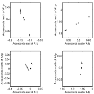
Figure 3: Observed and model positions for the images of MG J0414+0534. Clockwise from lower left, the panels show the vicinity of the images A1, A2, B and C. The model positions are plotted as small crosses ($\times$). The error ellipses represent the 90%-confidence intervals for the observed image positions. The large error ellipses were computed using the stat-width error estimates, whereas the small error ellipses (most of which appear pointlike on a plot of this scale) were computed using the statistical error estimates. The different error estimates are described in 4.1.

Table 7 contains a list of the best-fit parameters. In addition, Table 8 lists the image magnifications predicted by this best-fit model (which may be compared to the flux ratios in Table 1). Figure 3 shows both the observed and modeled image locations for each of the sixteen components of the VLBI map, along with the stat-width error ellipses.

In this model, the center of mass of the mass distribution interior to $r=b$ is located at $\Delta\alpha=-1\arcsec.0788\pm 0\arcsec.0020$, $\Delta\delta=0\arcsec.6635\pm 0\arcsec.0012$ relative to the correlation center at component A1p. Since the position of component Cp relative to the correlation center was $\Delta\alpha=-1\arcsec.9454$, $\Delta\delta=0\arcsec.3004$ (with position errors negligible compared to those of the model galaxy, see Table 1) the model center of mass is $\Delta\alpha=0\arcsec.8666\pm 0\arcsec.0020$, $\Delta\delta=0\arcsec.3631\pm 0\arcsec.0012$ relative to Cp. This is in agreement with the optical centroid of the lens galaxy as observed by Falco, Lehár & Shapiro (1997) even though the optical position was not used as a modeling constraint. The observed lens galaxy position in $R$-band, relative to component C, was $\Delta\alpha=0\arcsec.90\pm 0\arcsec.05$, $\Delta\delta=0\arcsec.32\pm 0\arcsec.05$; the observed position in $I$-band was $\Delta\alpha=0\arcsec.86\pm 0\arcsec.05$, $\Delta\delta=0\arcsec.36\pm 0\arcsec.05$.

As is apparent in Table 7 and Figure 5, the directions of mass excess implied by both the internal and external quadrupoles (${{\bf A}}_{2}^{\prime}$ and ${{\bf B}}_{2}^{\prime}$) agree with the direction of the optical isophotes ($71\arcdeg\pm 5\arcdeg$) observed by Falco, Leár & Shapiro (1997). Interestingly, one of the directions of mass deficit implied by the external $m=4$ multipole, ${{\bf A}}_{4}^{\prime}$, is also in agreement with the optical isophote angle. The eastern direction of the external octupole, ${{\bf A}}_{3}^{\prime}$, is aligned with the external quadrupole moment within $6\arcdeg$, and is within $10\arcdeg$ of the observed isophote angle, although in neither case do the formal confidence regions overlap. It is possible that the alignments between the multipole angles and the optical isophotes are coincidences. If the isophote angle were selected at random, the chance of agreement with the direction of mass-excess indicated by ${{\bf A}}_{2}^{\prime}$ would be $6\%$, given the quoted confidence ranges. The chance of agreement with the direction of either the mass excess or mass deficit implied by ${{\bf A}}_{4}^{\prime}$ would be 27%. The chance that ${{\bf A}}_{3}^{\prime}$ and the isophote angles would be as closely aligned as they are is 34%.

Bearing this in mind, we entertain three speculations regarding the origin of the external multipoles in the best-fit model $b+{{\bf A}}_{2}+{{\bf B}}_{2}+{{\bf A}}_{3}+{{\bf A}}_{4}$:

1. All of the external multipoles are attributable to the mass distribution of the lens galaxy. This explains the alignments of the various multipole angles with the optical isophotes, but it implies that no external perturber (i.e. neither object X nor the group of galaxies to the southwest) contributes significantly to the features of the potential we have modeled. A singular isothermal elliptical potential would have a ratio of external to internal quadrupole of $|{{\bf A}}_{2}|/|{{\bf B}}_{2}|=3$, which is consistent with the value $2.90\pm 0.17$ obtained for this model. The ellipticity ($1-b/a$) of the isopotential contours near the ring radius for the fitted model is $\epsilon_{\Phi}=2|{{\bf A}}_{2}^{\prime}+{{\bf B}}_{2}^{\prime}|=0.120\pm 0.002$. In contrast the ellipticity of a singular isothermal elliptical potential (SIEP) having an isodensity ellipticity of $\epsilon_{G}=0.20\pm 0.02$ (equal to the mean ellipticity of the fitted isophotes of Falco, Lehár & Shapiro (1997)) would be $\epsilon_{\Phi}=0.07$. However, the non-zero ${{\bf A}}_{3}^{\prime}$ implies that the outer galactic halo is asymmetric, with more mass concentrated near one end of the isophote axis than the other. Furthermore, the magnitude of ${{\bf A}}_{4}^{\prime}$ ($4.1\times 10^{-3}$) is an order of magnitude larger than the value it would assume for an singular isothermal elliptical potential ($6\times 10^{-4}$). The direction of ${{\bf A}}_{4}^{\prime}$ implies that the mass distribution is box-like, rather than disk-like as for a SIEP.

2. ${{\bf A}}_{2}^{\prime}$ and ${{\bf A}}_{3}^{\prime}$ indicate an external perturbing mass to the east. In this case the alignments of all multipoles with the isophotes are accidental. According to equation 51, a point mass with an Einstein radius of $0.95\pm 0.05$ arcseconds, located $3.2\pm 0.2$ arcseconds away, would supply approximately the appropriate values of ${{\bf A}}_{2}^{\prime}$ and ${{\bf A}}_{3}^{\prime}$, but would not account for ${{\bf A}}_{4}^{\prime}$. No perturber of any kind is seen to the east in the optical images of Falco, Lehár & Shapiro (1997).

3. ${{\bf A}}_{3}^{\prime}$ and ${{\bf A}}_{4}^{\prime}$ indicate an external perturbing mass at about $-65\arcdeg\pm 4\arcdeg$ N of W. In this case, as above, the alignments of all multipoles with the isophotes are accidental. A point mass $2.24\pm 0.24$ arcseconds away, with Einstein radius $0.56\pm 0.10$ arcseconds, would supply the proper $|{{\bf A}}_{3}|$ and $|{{\bf A}}_{4}|$, but would also make a significant contribution to ${{\bf A}}_{2}$. The residual component of ${{\bf A}}_{2}^{\prime}$, which would presumably be due to the lensing galaxy, has magnitude 0.06 and direction $1.5\arcdeg$ or $181.5\arcdeg$ north of west. This is somewhat problematic because the residual quadrupole does not agree in angle with the optical isophotes, and its magnitude is uncomfortably large ($|{{\bf A}}_{2}^{\prime}|/|{{\bf B}}_{2}^{\prime}|=3.8$). However, there is an object seen in the optical image of Falco, Lehár & Shapiro (1997) about $5\arcsec$ away in the direction $-54\arcdeg$ N of W.

None of these speculations is entirely satisfactory. The first speculation attributes a peculiar shape to the galactic halo; the second invokes an external perturber that does not seem to be present; the third compels the galaxy to produce an unusual quadrupole moment. We favor the first interpretation, because it is hard to arrange for an external perturbation to produce ${{\bf A}}_{3}^{\prime}$ without ruining the suggestive alignment of ${{\bf A}}_{2}^{\prime}$ with the isophotes, but admit that this interpretation is debatable.

This ambiguity of interpretation illustrates both the appeal and the frustration of the multipole-Taylor technique for modeling lens potentials. The technique makes few preconceptions about the shape of the potential, which in principle may lead to unanticipated discoveries about the mass distribution of the deflector, including the shape of the halo (of which little is presently known). However, precisely because of this mathematical generality, there is no determinative way to correlate features of the potential with observed astrophysical objects (the lens galaxy or external perturbers).

Finally, we comment on the unconstrainability of the radial distribution of the mass monopole. It is not terribly surprising that we were unable to usefully constrain the parameter $f_{3}^{\prime}$, the lowest-order parameter containing information about the radial distribution. A large change in $f_{3}^{\prime}$ is needed to cause a small change in the radial positions of images near the ring radius. By contrast, even small values of ${{\bf A}}_{m}^{\prime}$ or ${{\bf B}}_{m}^{\prime}$ (for $m\geq 2$) cause shifts in the radial positions of images near the ring radius. In particular, varying ${{\bf A}}_{m}^{\prime}$ and ${{\bf B}}_{m}^{\prime}$ while leaving their sum unchanged affects the radial image displacements, but has little effect on the tangential image displacements (see Table 3). The radial image shifts caused by these multipole terms depend on angular position, whereas those caused by $f_{3}^{\prime}$ do not. However, for lenses such as MG J0414+0534, in which there are only images at a few angular locations, the effects of $f_{3}^{\prime}$ and of ${{\bf A}}_{m}^{\prime}$ or ${{\bf B}}_{m}^{\prime}$ may compete, with large changes in $f_{3}^{\prime}$ compensating for small changes in ${{\bf A}}_{m}^{\prime}$ or ${{\bf B}}_{m}^{\prime}$. For systems with arcs or rings of lensed emission, information is available from a broader range of angles. The optical arc visible in MG J0414+0534 (Falco, Lehár & Shapiro (1997)) may further constrain MG J0414+0534’s angular multipole moments, especially if its location can be measured with the same precision as the VLBA measurements used in this paper.

That the radial profile parameter, $f_{3}^{\prime}$, is so difficult to determine is unfortunate. It would provide information on how the angularly-averaged surface mass density decreases with radius near the Einstein ring radius, which could be used help choose a model value for $\sigma_{0}(b)$. The quantity $\sigma_{0}(b)$ is not directly constrainable from lensing, but it does affects the predicted time delays between images, a topic discussed in the next section.

5.2 Implications for the time delays

Each of the multiple images formed by a gravitational lens represents the source object at a different moment in its history. This is because the propagation time from source to observer is different for each image, due to the different path lengths and Shapiro delays experienced by the ray bundles composing each image. In particular, the time delay by which an image at ${\bf r}_{\alpha}$ lags that at ${\bf r}_{\beta}$ is, as computed by Narayan & Bartelmann (1996),

$$\Delta t_{\beta\alpha}=t({\bf r}_{\alpha})-t({\bf r}_{\beta})=(1+z_{l})\frac{D_{L}D_{S}}{D_{LS}}\left(\frac{1}{2}|{\mbox{\boldmath{$\nabla$}}}_{{\bf r}_{\alpha}}\Phi({\bf r}_{\alpha})|^{2}-\frac{1}{2}|{\mbox{\boldmath{$\nabla$}}}_{{\bf r}_{\beta}}\Phi({\bf r}_{\beta})|^{2}-\Phi({\bf r}_{\alpha})+\Phi({\bf r}_{\beta})\right)$$ (62)

It is convenient to define a “dimensionless time delay” $\Delta\tau_{\beta\alpha}$ which depends only on the modeled lens potential and requires no values for redshifts or cosmological parameters,

$$\Delta\tau_{\beta\alpha}=\frac{1}{2}|{\mbox{\boldmath{$\nabla$}}}_{{\bf r}_{\alpha}}\Phi({\bf r}_{\alpha})|^{2}-\frac{1}{2}|{\mbox{\boldmath{$\nabla$}}}_{{\bf r}_{\beta}}\Phi({\bf r}_{\beta})|^{2}-\Phi({\bf r}_{\alpha})+\Phi({\bf r}_{\beta})$$ (63)

and which is related to the time delay by a conversion factor depending on the redshifts and cosmology,

$$\Delta t_{\beta\alpha}=(1+z_{l})\frac{D_{L}D_{S}}{D_{LS}}\Delta\tau_{\beta\alpha}.$$ (64)

A measurement of the time delay between the flux variations in corresponding images and the lens redshift $z_{l}$, when combined with a model that predicts the dimensionless time delay, thereby amounts to a measurement of the combination of angular diameter distances $D_{L}D_{S}/D_{LS}$. Since the relation between angular diameter distance and redshift depends on the values of $H_{0}$, $\Omega_{m}$, and $\Omega_{\Lambda}$, these cosmological parameters can be thereby constrained. The appeal of this well-known cosmological probe is that it does not rely on the usual intermediate distance indicators (Refsdal 1964, (1966)).

One problem with this idea arises from the mass-sheet degeneracy, which was discussed in section 3.4. When the potential is transformed by the mass sheet degeneracy, the time delays between components are likewise transformed. Using the model potential of equation 3.4, the model dimensionless time delay, $\Delta\tau^{\prime}$, is related to the true dimensionless time delay, $\Delta\tau$, by

$$\Delta\tau^{\prime}_{\alpha\beta}=\frac{1}{2\left(1-\frac{\sigma_{0}(b)}{{\sigma_{\rm c}}}\right)}\Delta\tau_{\alpha\beta}$$ (65)

where $\sigma_{0}(b)$ is the angularly-averaged surface mass density at the Einstein ring radius. Unless the mass-sheet degeneracy can be resolved by determining $\sigma_{0}(b)/{\sigma_{\rm c}}$ in some independent fashion the time delays cannot be predicted, although the ratios of time delays between different image pairs can still be predicted.

Although MG J0414+0534 has been extensively monitored at radio wavelengths, no flux variations have been observed that are large enough to permit an accurate time delay measurement (Moore & Hewitt (1997)). Nevertheless, this does not preclude radio or optical detections of time delays in the future, so it is important to understand how our models of MG J0414+0534 constrain the time delays. As discussed in the previous section, the best-fit model was $b+{{\bf A}}_{2}+{{\bf B}}_{2}+{{\bf A}}_{3}+{{\bf A}}_{4}$. We used this model to make our single best prediction for the time delays of MG J0414+0534, by computing the dimensionless time delays between the 4 images of the brightest component (p).

The uncertainty in this particular model’s predicted time delay due to the uncertainty in the measured image positions was estimated in the following manner. We re-computed the time delay with each parameter (one at a time) adjusted to its maximum and minimum values allowed by the stat-width confidence limits, while minimizing the $\chi^{2}$ over all the other parameters. The range between the highest and lowest time delays that were achieved during these parameter-by-parameter adjustments is our estimate for the uncertainty in the time delay for that particular model.

However, we must also take into account the larger uncertainty in the predicted time delay caused by the uncertain choice of model. To estimate this uncertainty, we computed dimensionless time delays for a large subset of the models that were discussed in the previous section. For the 11-parameter and 12-parameter models, we included models which adequately fit the observations when using the stat-width error estimates ($N_{\sigma}<3$). The $+{{\bf A}}_{3}+{{{\bf M}}^{\rm sum}_{4}}+f_{3}$ and $+{{\bf A}}_{3}+{{\bf B}}_{4}+f_{3}$ models were excluded because, for these models, the entire confidence range for $f^{\prime}_{3}$ lies above $f^{\prime}_{3}>2$, well within the unphysical region $f^{\prime}_{3}>1$. Likewise, the $+{{\bf A}}_{3}+{{\bf G}}_{22}$ model was not included because of its unphysically large value of $|{{\bf G}}^{\prime}_{22}|$, as discussed in section 4.2. The results are shown in Table 9. Since these models make somewhat different predictions, any attempt to make a single prediction for the time delays must incorporate the uncertainty associated with the selection of a single model. Thus we have enlarged the error spread in our best predictions for the time delays to include the whole range of time delays predicted by all these models. The resulting predictions are:

$$\Delta\tau_{BA}^{\prime}=\frac{1}{2\left(1-\frac{\sigma_{0}(b)}{{\sigma_{\rm c}}}\right)}\Delta\tau_{BA} = 1.828\times 10^{-12}\,\left[1{}^{+}_{-}\underbrace{{}^{0.020}_{0.018}}_{\begin{array}[t]{@{}l@{}}{\scriptscriptstyle\rm formal}\\ {\scriptscriptstyle\rm errors\rule{0.0pt}{2.15277pt}}\end{array}}\pm\underbrace{0.014}_{\begin{array}[t]{@{}l@{}}{\scriptscriptstyle\rm A1-A2}\\ {\scriptscriptstyle\rm difference\rule{0.0pt}{2.15277pt}}\end{array}}{}^{+}_{-}\underbrace{{}^{0.616}_{0.038}}_{\begin{array}[t]{@{}l@{}}{\scriptscriptstyle\rm which}\\ {\scriptscriptstyle\rm model\rule{0.0pt}{2.15277pt}}\end{array}}\right],$$ (72)

$$\Delta\tau_{AC}^{\prime}=\frac{1}{2\left(1-\frac{\sigma_{0}(b)}{{\sigma_{\rm c}}}\right)}\Delta\tau_{AC} = 1.042\times 10^{-11}\,\left[1\pm\underbrace{0.017}_{\begin{array}[t]{@{}l@{}}{\scriptscriptstyle\rm formal}\\ {\scriptscriptstyle\rm errors\rule{0.0pt}{2.15277pt}}\end{array}}\pm\underbrace{0.002}_{\begin{array}[t]{@{}l@{}}{\scriptscriptstyle\rm A1-A2}\\ {\scriptscriptstyle\rm difference\rule{0.0pt}{2.15277pt}}\end{array}}{}^{+}_{-}\underbrace{{}^{0.085}_{0.198}}_{\begin{array}[t]{@{}l@{}}{\scriptscriptstyle\rm which}\\ {\scriptscriptstyle\rm model\rule{0.0pt}{2.15277pt}}\end{array}}\right],$$ (79)

$$\Delta\tau_{BC}^{\prime}=\frac{1}{2\left(1-\frac{\sigma_{0}(b)}{{\sigma_{\rm c}}}\right)}\Delta\tau_{BC} = 1.225\times 10^{-11}\,\left[1\pm\underbrace{0.017}_{\begin{array}[t]{@{}l@{}}{\scriptscriptstyle\rm formal}\\ {\scriptscriptstyle\rm errors\rule{0.0pt}{2.15277pt}}\end{array}}{}^{+}_{-}\underbrace{{}^{0.138}_{0.148}}_{\begin{array}[t]{@{}l@{}}{\scriptscriptstyle\rm which}\\ {\scriptscriptstyle\rm model\rule{0.0pt}{2.15277pt}}\end{array}}\right].$$ (84)

Here the “formal errors” represent the uncertainty in the parameters of the best-fit model, the “A1-A2 difference” is half the time delay between images A1 and A2 (since the joint A1-A2 light curve would probably be used to measure time delays), and “which model” refers to the uncertainty due to choice of model. The factor $2\left(1-{\sigma_{0}(b)}/{{\sigma_{\rm c}}}\right)$ represents the uncertainty in the time delay due to the mass-sheet degeneracy, which can only be relieved by obtaining a reliable value of ${\sigma_{0}(b)}/{{\sigma_{\rm c}}}$ from other observational or theoretical sources. For a potential with the radial profile of an isothermal sphere, $2\left(1-{\sigma_{0}(b)}/{{\sigma_{\rm c}}}\right)=1$.

To express the time delay as an actual number of days, the conversion factor of equation 64 must be used. For MG J0414+0534, which has $z_{l}=0.9584$ and $z_{s}=2.639$, this conversion factor takes the value $\Delta t/\Delta\tau=6.794\times 10^{12}\,h_{75}^{-1}$ days, assuming the universe has $\Omega_{m}=1$, $\Omega_{\Lambda}=0$, and $H_{0}=75h_{75}$ km/s/Mpc. The values of this conversion factor for some other choices of cosmological parameters are tabulated in Table 10. In all cases, the “filled-beam” approximation was used to compute the conversion factor, in which the universe is assumed to have a perfectly smooth distribution of matter. The presence of clumpiness would require the angular-diameter distances to be re-computed (see e.g. Fukugita et al. (1992)).

A promising way to reduce the “which model” uncertainty is to measure the time delay ratio $\Delta t_{AB}/\Delta t_{AC}$. Predictions for this ratio are presented in Table 11 for various models. If this quantity is in accordance with the prediction of our best-fit model $b+{{\bf A}}_{2}+{{\bf B}}_{2}+{{\bf A}}_{3}+{{\bf A}}_{4}$, and it can be measured to within 3%, then it would exclude all the other models listed and the “which model” error would fall away. Even if the ratio could only be measured to within 18%, it would exclude all but one other model, which would shrink the “which model” uncertainty in $\Delta t_{AB}$ to only 3.7% (from 62%). In this scenario, and using the conversion factor (eq. 64) for $\Omega_{m}=1$, $\Omega_{\Lambda}=0$, we would predict

$$\left.\begin{array}[]{ccl}H_{0}&=&75\,{\rm km/s/Mpc}\,\frac{12.42\,\rm days}{\Delta t_{BA}}\,\left[1{}^{+}_{-}\underbrace{{}^{0.020}_{0.018}}_{\begin{array}[t]{@{}l@{}}{\scriptscriptstyle\rm formal}\\ {\scriptscriptstyle\rm errors\rule{0.0pt}{2.15277pt}}\end{array}}\pm\underbrace{0.014}_{\begin{array}[t]{@{}l@{}}{\scriptscriptstyle\rm A1-A2}\\ {\scriptscriptstyle\rm difference\rule{0.0pt}{2.15277pt}}\end{array}}{}^{+}_{-}\underbrace{{}^{0.000}_{0.037}}_{\begin{array}[t]{@{}l@{}}{\scriptscriptstyle\rm which}\\ {\scriptscriptstyle\rm model\rule{0.0pt}{2.15277pt}}\end{array}}\right]\left[{2\left(1-\frac{\sigma_{0}(b)}{{\sigma_{\rm c}}}\right)}\right]\\ H_{0}&=&75\,{\rm km/s/Mpc}\,\frac{70.79\,\rm days}{\Delta t_{AC}}\,\left[1\pm\underbrace{0.017}_{\begin{array}[t]{@{}l@{}}{\scriptscriptstyle\rm formal}\\ {\scriptscriptstyle\rm errors\rule{0.0pt}{2.15277pt}}\end{array}}\pm\underbrace{0.002}_{\begin{array}[t]{@{}l@{}}{\scriptscriptstyle\rm A1-A2}\\ {\scriptscriptstyle\rm difference\rule{0.0pt}{2.15277pt}}\end{array}}{}^{+}_{-}\underbrace{{}^{0.000}_{0.111}}_{\begin{array}[t]{@{}l@{}}{\scriptscriptstyle\rm which}\\ {\scriptscriptstyle\rm model\rule{0.0pt}{2.15277pt}}\end{array}}\right]\left[{2\left(1-\frac{\sigma_{0}(b)}{{\sigma_{\rm c}}}\right)}\right]\\ H_{0}&=&75\,{\rm km/s/Mpc}\,\frac{83.23\,\rm days}{\Delta t_{BC}}\,\left[1\pm\underbrace{0.017}_{\begin{array}[t]{@{}l@{}}{\scriptscriptstyle\rm formal}\\ {\scriptscriptstyle\rm errors\rule{0.0pt}{2.15277pt}}\end{array}}{}^{+}_{-}\underbrace{{}^{0.000}_{0.100}}_{\begin{array}[t]{@{}l@{}}{\scriptscriptstyle\rm which}\\ {\scriptscriptstyle\rm model\rule{0.0pt}{2.15277pt}}\end{array}}\right]\left[{2\left(1-\frac{\sigma_{0}(b)}{{\sigma_{\rm c}}}\right)}\right]\end{array}\right\}\rule{5.0pt}{0.0pt}\parbox{78.04842pt}{ Assuming the time delay ratio is measured to within $\sim$18\% and agrees with our best-fit model.}$$ (85)

6 Conclusions

Upon first seeing the rich sub-structure in each VLBI image of MG J0414+0534, we were hopeful that such a large body of precise constraints on the modeling potential would lead to tight constraints on the mass distribution of the deflector and the predicted time delays between images. We hoped that the mathematical generality of the multipole-Taylor expansion (with slight modifications) would allow us to draw such conclusions without contamination from (perhaps faulty) astrophysical preconceptions. These hopes were only partly fulfilled.

Once the best-fit parameters in the expansion are determined, it is difficult to know from which astrophysical source they arise. For example, our best-fit model $b+{{\bf A}}_{2}+{{\bf B}}_{2}+{{\bf A}}_{3}+{{\bf A}}_{4}$ seems to imply that either the mass distribution in the lensing galaxy is asymmetric and somewhat quadrangular (boxy), or else that an unseen external perturber is partly responsible for the light deflection (as discussed in section 5.1). It is possible, however, that the values of the best-fit model parameters may guide future interpretations of observations for this system, by indicating the possible directions of perturbing masses.

Predictions of time delays, while quite well-constrained for any particular model potential, are limited by the uncertainty in selecting one of several viable models. In other words, the predictions are not limited by the precision of the positional constraints, but rather by the ability to satisfy those constraints with several alternative truncations of the multipole-Taylor series. In the case of MG J0414+0534, we found that one way to relieve this crucial source of systematic error is to measure ratios of time delays, which are predicted to have different values by different models.

Despite these limitations, which afflict all lens modeling techniques to date, the multipole-Taylor expansion does indeed seem to be an appropriate form for multiple-image gravitational lenses such as MG J0414+0534. The simplest three-term truncation reproduces the observed image configuration far better than previously-used simpler models, and successively higher terms improve the fit by incrementally smaller amounts. The radial profile parameter $f^{\prime}_{3}$ could not be constrained, but this is likely to be the case for any point-modeling scheme applied to quadruple-image lenses.

We believe the multipole-Taylor expansion could be usefully applied to other lenses in which the constraints occur at locations close to the Einstein radius, and the angular variation of the potential is expected to be fairly smooth. One serious problem with the efforts to date to determine $H_{0}$ and other cosmological parameters by measuring time delays is that each known gravitational lens has usually been modeled in an individual and idiosyncratic manner. The multipole-Taylor expansion is one candidate for a very general modeling technique that could be applied to all the time-delay lenses, so that the results of these efforts could be sensibly combined.

Figure 2: High-resolution maps of the four images of MG J0414+0534, observed at 5 GHz with the VLBA, are shown with the four components p, q, r and s identified. The positions and fluxes for these components are reported in Table 1.

Figure 4: Model $b+{{\bf A}}_{2}+{{\bf B}}_{2}+{{\bf A}}_{3}$, fitted to MG J0414+0534. The model parameters are illustrated graphically. North is up and east is left. An $\times$ marks the model deflector center of mass $(g_{x},g_{y})$, and a ring is drawn at the model Einstein ring radius $b$. The error range on the ring radius is shown by additional rings drawn at the upper and lower confidence limits. (At this plot scale, neither the error rings nor the error range for the model galaxy position can be resolved.) Each $m\geq 1$ multipole moment is illustrated by arrows pointing in the possible directions to mass excesses that would cause such a multipole moment. The arrows are labeled with the number $m$ of the multipole moment, and their lengths are proportional to the amplitudes of the multipole moments. Confidence ranges on the angles are indicated by small arcs at the tip of each arrow. Also shown are the $R$ and $I$-band center positions of the deflector galaxy ($+$ marks), the position of Object X, the direction to a nearby group of galaxies (arrow), and the orientation of the galaxy isophotes (arcs near the ring radius), all from Falco, Lehár & Shapiro (1997) The locations of the observed and modeled components are also shown but cannot be distinguished at this plot scale. See Figure 3 for a closer view. The model sources are plotted northeast of the galaxy center.

Figure 5: Model $b+{{\bf A}}_{2}+{{\bf B}}_{2}+{{\bf A}}_{3}+{{\bf A}}_{4}$, fitted to MG J0414+0534. The model parameters are illustrated graphically, using the same conventions as in Figure 4.

	Component location		Centroid errors			Peak flux	Integral flux
	$x=-\mbox{R.A.}$	$y=\mbox{Dec.}$	$\sigma_{x}$	$\sigma_{y}$	$\sigma_{xy}^{2}$	(mJy/beam)	(mJy)
	(mas)	(mas)	(mas)	(mas)	(mas2)
A1p	0.0144	0.3818	0.0018	0.0037	-2.33e-6	$108.1\pm 0.2$	$149.1\pm 0.4$
A2p	-134.0714	405.9972	0.0025	0.0062	-7.09e-6	$88.0\pm 0.3$	$125.9\pm 0.5$
Bp	588.6037	1938.3514	0.0056	0.0089	8.09e-6	$33.2\pm 0.2$	$43.4\pm 0.4$
Cp	1945.3597	300.4118	0.0061	0.0156	6.06e-6	$20.5\pm 0.2$	$22.5\pm 0.3$
A1q	1.9438	1.6872	0.0044	0.0103	-9.76e-6	$39.2\pm 0.2$	$48.8\pm 0.4$
A2q	-130.5108	397.7602	0.0075	0.0195	-7.12e-5	$28.1\pm 0.3$	$39.2\pm 0.5$
Bq	598.4155	1943.2536	0.0215	0.0263	1.53e-4	$10.7\pm 0.2$	$17.5\pm 0.4$
Cq	1944.7253	296.2398	0.0203	0.0401	2.22e-4	$6.5\pm 0.2$	$6.6\pm 0.3$
A1r	6.7992	21.2226	0.0298	0.0563	-1.30e-3	$9.2\pm 0.2$	$20.2\pm 0.6$
A2r	-104.5880	332.3330	0.0243	0.0770	-1.31e-3	$10.1\pm 0.2$	$22.7\pm 0.7$
Br	652.1233	1970.6440	0.0356	0.0626	1.69e-4	$5.2\pm 0.2$	$7.1\pm 0.4$
Cr	1939.5305	271.3034	0.0365	0.1004	2.01e-6	$2.7\pm 0.2$	$2.5\pm 0.2$
A1s	-16.1756	6.1174	0.0854	0.1362	-1.13e-2	$6.6\pm 0.1$	$61.6\pm 1.2$
A2s	-149.3272	432.3058	0.0236	0.1334	-9.98e-4	$8.4\pm 0.2$	$49.7\pm 1.2$
Bs	536.6837	1912.7346	0.0978	0.0561	3.02e-3	$4.2\pm 0.1$	$17.5\pm 0.7$
Cs	1945.9419	319.7664	0.0617	0.1036	-4.45e-3	$4.4\pm 0.2$	$15.2\pm 0.6$

Table 1: Centroid locations and flux densities of the elliptical Gaussian fits to the components of MG J0414+0534, derived from the VLBA observations described by Trotter (1998). The positions are relative to the correlation and fringe-fitting center at A1. The $x$-coordinate increases to the west and the $y$-coordinate increases to the north. The errors on the centroid positions are standard deviations on the $x$- and $y$-positions due to the thermal noise in the map, and the corresponding correlation between the $x$- and $y$-position errors. The flux errors are standard deviations due to the thermal noise in the map. These error bars do not include the effect of deconvolution error.

Multipole moment $m$	Radial dependence	Parameter	Significance
$\cdots$	$\cdots$	$g_{x}$, $g_{y}$	Location of origin.
$m=0$	$t=0$	$f_{0}$	Constant offset (unconstrainable).
$m=0$	$t=1$	$b$	Einstein ring radius. Sensitive to total mass within ring.
$m=0$	$t=2$	$f_{2}$	Sets surface mass density at ring, $\sigma_{0}(b)$ (unconstrainable due to mass-sheet degeneracy).
$m=0$	$t\geq 3$	$f_{t}$	Depends on $\sigma_{0}(r)$ and its derivatives near $r=b$. For $t=3$, gives falloff of surface mass density with radius, evaluated at the ring radius. See Eq. 44.
$m=1$	exterior	${{\bf A}}_{1}$	Dipole moment of mass exterior to ring (unconstrainable due to prismatic degeneracy).
$m\geq 2$	exterior	${{\bf A}}_{m}$	Sensitive to multipole moment of mass exterior to ring.
$m=1$	interior	${{\bf B}}_{1}$	Sets COM of mass interior to ring. (The COM may be placed at the origin by setting ${{\bf B}}_{1}=0$.)
$m\geq 2$	interior	${{\bf B}}_{m}$	Sensitive to multipole moment of mass interior to ring.
$m\geq 1$	$t\geq 2$	${{\bf G}}_{mt}$	Depends on ${\mbox{\boldmath$\sigma$}}_{m}(r)$ and its derivatives near $r=b$.
$m\geq 2$	$t=0$	${{{\bf M}}^{\rm sum}_{m}}$	${{{\bf M}}^{\rm sum}_{m}}={{\bf A}}_{m}+{{\bf B}}_{m}$, sum of external and internal mass multipoles. (This parameter is from the parameterization in equation 7, rather than equation 47).

Table 2: Physical significance of the parameters and terms in the modified multipole-Taylor series, equation 47. The first column lists the multipole moment $m$. The second column describes the radial dependence (the exponent $t$ of $\rho^{t}$, or whether the term is sensitive to mass interior or exterior to $r=b$). The third column lists the name of the parameter. The last column describes the physical significance of the term. The parameters $f_{0}$, $f_{2}$, ${{\bf A}}_{1}$, and ${{\bf B}}_{1}$ cannot be constrained from lensing, as explained in section 3.4. We set these parameters equal to zero during the model-fitting procedure.

$m$	$t$	$\frac{1}{b}{\mbox{\boldmath{$\nabla$}}}_{{\bf r}}\Phi^{\prime}$	Image Displacements
$m=0$	$t=0$	$0$	None
$m=0$	$t=1$	${\hat{\bf r}}$	Radial
$m=0$	$t\geq 2$	${\hat{\bf r}}\left\{\frac{1}{(t-1)!}\rho^{(t-1)}\right\}\left\{f_{t}^{\prime}\right\}$	Small, radial
$m\geq 1$	exterior	$\begin{array}[t]{c}{\hat{\bf r}}\left\{-m(1+\rho)^{(m-1)}\right\}\left\{{A_{m{\rm c}}^{\prime}\cos m\theta+A_{m{\rm s}}^{\prime}\sin m\theta}\right\}\\ +{\hat{\mbox{\boldmath$\theta$}}}\left\{m(1+\rho)^{(m-1)}\right\}\left\{{A_{m{\rm c}}^{\prime}\sin m\theta-A_{m{\rm s}}^{\prime}\cos m\theta}\right\}\end{array}$	Radial and tangential
$m\geq 1$	interior	$\begin{array}[t]{c}{\hat{\bf r}}\left\{\frac{m}{(1+\rho)^{(m+1)}}\right\}\left\{{B_{m{\rm c}}^{\prime}\cos m\theta+B_{m{\rm s}}^{\prime}\sin m\theta}\right\}\\ +{\hat{\mbox{\boldmath$\theta$}}}\left\{\frac{m}{(1+\rho)^{(m+1)}}\right\}\left\{{B_{m{\rm c}}^{\prime}\sin m\theta-B_{m{\rm s}}^{\prime}\cos m\theta}\right\}\end{array}$	Radial and tangential
$m\geq 1$	$t\geq 2$	$\begin{array}[t]{c}{\hat{\bf r}}\left\{\frac{\rho^{(t-1)}}{(t-1)!}\right\}\left\{{G_{mt{\rm c}}^{\prime}\cos m\theta+G_{mt{\rm s}}^{\prime}\sin m\theta}\right\}\\ +{\hat{\mbox{\boldmath$\theta$}}}\left\{-\frac{m}{t!}\frac{\rho^{t}}{(1+\rho)}\right\}\left\{{G_{mt{\rm c}}^{\prime}\sin m\theta-G_{mt{\rm s}}^{\prime}\cos m\theta}\right\}\end{array}$	Small, predominantly radial
$m\geq 1$	$t=0$	${\hat{\mbox{\boldmath$\theta$}}}\left\{\frac{m}{1+\rho}\right\}\left\{{{M^{\rm sum}_{{m{\rm c}}}}^{\prime}\sin m\theta-{M^{\rm sum}_{{m{\rm s}}}}^{\prime}\cos m\theta}\right\}$	Tangential, due to overall strength of multipole ${{{\bf M}}^{\rm sum}_{m}}^{\prime}={{\bf A}}_{m}^{\prime}+{{\bf B}}_{m}^{\prime}$
$m\geq 1$	$t=1$	$\begin{array}[t]{c}{\hat{\bf r}}\left\{-m\right\}\left\{{{M^{\rm diff}_{{m{\rm c}}}}^{\prime}\cos m\theta+{M^{\rm diff}_{{m{\rm s}}}}^{\prime}\sin m\theta}\right\}\\ +{\hat{\mbox{\boldmath$\theta$}}}\left\{\frac{\rho m^{2}}{1+\rho}\right\}\left\{{{M^{\rm diff}_{{m{\rm c}}}}^{\prime}\sin m\theta-{M^{\rm diff}_{{m{\rm s}}}}^{\prime}\cos m\theta}\right\}\end{array}$	Predominantly radial. Affected by balance between external and internal multipole ${{{\bf M}}^{\rm diff}_{m}}^{\prime}={{\bf A}}_{m}^{\prime}-{{\bf B}}_{m}^{\prime}$

Table 3: The first derivatives of the terms in our parameterization of the lens potential. These are needed to calculate the displacement of the lens images from the source positions (eq. 3). The upper section of the table lists the five functional forms needed to represent the terms in the modified multipole-Taylor expansion of the potential (eq. 47). The lower section of the table lists functional forms for terms in the original expansion (eq. 7). The identifications $m$ and $t$ are as in Table 2. The model parameters are written in Cartesian form, e.g. ${{\bf A}}_{m}^{\prime}={\hat{\bf x}}A_{m{\rm c}}^{\prime}+{\hat{\bf y}}A_{m{\rm s}}^{\prime}$.

$m$	$t$	${\mbox{\boldmath{$\nabla$}}}_{{\bf r}}{\mbox{\boldmath{$\nabla$}}}_{{\bf r}}\Phi^{\prime}$
$m=0$	$t=0$	0
$m=0$	$t=1$	${\hat{\mbox{\boldmath$\theta$}}}{\hat{\mbox{\boldmath$\theta$}}}\left\{\frac{1}{1+\rho}\right\}$
$m=0$	$t\geq 2$	$\begin{array}[t]{c}{\hat{\bf r}}{\hat{\bf r}}\left\{\frac{1}{(t-2)!}\rho^{(t-2)}\right\}\left\{f_{t}^{\prime}\right\}\\ +{\hat{\mbox{\boldmath$\theta$}}}{\hat{\mbox{\boldmath$\theta$}}}\left\{\frac{1}{(t-1)!}\frac{\rho^{(t-1)}}{(1+\rho)}\right\}\left\{f_{t}^{\prime}\right\}\end{array}$
$m\geq 1$	exterior	$\begin{array}[t]{c}{\hat{\bf r}}{\hat{\bf r}}\left\{-m(m-1)(1+\rho)^{(m-2)}\right\}\left\{{A_{m{\rm c}}^{\prime}\cos m\theta+A_{m{\rm s}}^{\prime}\sin m\theta}\right\}\\ +{\hat{\mbox{\boldmath$\theta$}}}{\hat{\mbox{\boldmath$\theta$}}}\left\{m(m-1)(1+\rho)^{(m-2)}\right\}\left\{{A_{m{\rm c}}^{\prime}\cos m\theta+A_{m{\rm s}}^{\prime}\sin m\theta}\right\}\\ +({\hat{\bf r}}{\hat{\mbox{\boldmath$\theta$}}}+{\hat{\mbox{\boldmath$\theta$}}}{\hat{\bf r}})\left\{m(m-1)(1+\rho)^{(m-2)}\right\}\left\{{A_{m{\rm c}}^{\prime}\sin m\theta-A_{m{\rm s}}^{\prime}\cos m\theta}\right\}\end{array}$
$m\geq 1$	interior	$\begin{array}[t]{c}{\hat{\bf r}}{\hat{\bf r}}\left\{-\frac{m(m+1)}{(1+\rho)^{(m+2)}}\right\}\left\{{B_{m{\rm c}}^{\prime}\cos m\theta+B_{m{\rm s}}^{\prime}\sin m\theta}\right\}\\ +{\hat{\mbox{\boldmath$\theta$}}}{\hat{\mbox{\boldmath$\theta$}}}\left\{\frac{m(m+1)}{(1+\rho)^{(m+2)}}\right\}\left\{{B_{m{\rm c}}^{\prime}\cos m\theta+B_{m{\rm s}}^{\prime}\sin m\theta}\right\}\\ +({\hat{\bf r}}{\hat{\mbox{\boldmath$\theta$}}}+{\hat{\mbox{\boldmath$\theta$}}}{\hat{\bf r}})\left\{-\frac{m(m+1)}{(1+\rho)^{(m+2)}}\right\}\left\{{B_{m{\rm c}}^{\prime}\sin m\theta-B_{m{\rm s}}^{\prime}\cos m\theta}\right\}\end{array}$
$m\geq 1$	$t\geq 2$	$\begin{array}[t]{c}{\hat{\bf r}}{\hat{\bf r}}\left\{\frac{\rho^{(t-2)}}{(t-2)!}\right\}\left\{{G_{mt{\rm c}}^{\prime}\cos m\theta+G_{mt{\rm s}}^{\prime}\sin m\theta}\right\}\\ +{\hat{\mbox{\boldmath$\theta$}}}{\hat{\mbox{\boldmath$\theta$}}}\left\{\frac{1}{t!}\frac{\rho^{(t-1)}}{(1+\rho)^{2}}(t-(m^{2}-t)\rho)\right\}\left\{{G_{mt{\rm c}}^{\prime}\cos m\theta+G_{mt{\rm s}}^{\prime}\sin m\theta}\right\}\\ +({\hat{\bf r}}{\hat{\mbox{\boldmath$\theta$}}}+{\hat{\mbox{\boldmath$\theta$}}}{\hat{\bf r}})\left\{-\frac{m}{t!}\frac{\rho^{(t-1)}}{(1+\rho)^{2}}(t+(t-1)\rho)\right\}\left\{{G_{mt{\rm c}}^{\prime}\sin m\theta-G_{mt{\rm s}}^{\prime}\cos m\theta}\right\}\end{array}$
$m\geq 1$	$t=0$	$\begin{array}[t]{c}{\hat{\mbox{\boldmath$\theta$}}}{\hat{\mbox{\boldmath$\theta$}}}\left\{\frac{m^{2}}{(1+\rho)^{2}}\right\}\left\{{{M^{\rm sum}_{{m{\rm c}}}}^{\prime}\cos m\theta+{M^{\rm sum}_{{m{\rm s}}}}^{\prime}\sin m\theta}\right\}\\ +({\hat{\bf r}}{\hat{\mbox{\boldmath$\theta$}}}+{\hat{\mbox{\boldmath$\theta$}}}{\hat{\bf r}})\left\{-\frac{m}{(1+\rho)^{2}}\right\}\left\{{{M^{\rm sum}_{{m{\rm c}}}}^{\prime}\sin m\theta-{M^{\rm sum}_{{m{\rm s}}}}^{\prime}\cos m\theta}\right\}\end{array}$
$m\geq 1$	$t=1$	$\begin{array}[t]{c}{\hat{\mbox{\boldmath$\theta$}}}{\hat{\mbox{\boldmath$\theta$}}}\left\{-\frac{m}{(1+\rho)^{2}}\left(1-(m^{2}-1)\rho\right)\right\}\left\{{{M^{\rm diff}_{{m{\rm c}}}}^{\prime}\cos m\theta+{M^{\rm diff}_{{m{\rm s}}}}^{\prime}\sin m\theta}\right\}\\ +({\hat{\bf r}}{\hat{\mbox{\boldmath$\theta$}}}+{\hat{\mbox{\boldmath$\theta$}}}{\hat{\bf r}})\left\{\frac{m^{2}}{(1+\rho)^{2}}\right\}\left\{{{M^{\rm diff}_{{m{\rm c}}}}^{\prime}\sin m\theta-{M^{\rm diff}_{{m{\rm s}}}}^{\prime}\cos m\theta}\right\}\end{array}$

Table 4: The second derivatives of the terms in our parameterization of the lens potential. These are needed for calculation of the magnification matrix. The notation is that of Table 3. The magnitude of the effect of each term on the inverse magnification matrix (eq. 55), may be seen by considering the exponent of $\rho$.

Model	$\Phi({\bf r})$	$\frac{\sigma_{0}(b)}{{\sigma_{\rm c}}}$	$1-\kappa=\frac{1}{2\left(1-\frac{\sigma_{0}(b)}{{\sigma_{\rm c}}}\right)}$	$f_{3}^{\prime}$
point mass	$b^{2}\ln r$	0	$1/2$	1
singular isothermal sphere	$br$	$1/2$	1	0
mass sheet with $\sigma={\sigma_{\rm c}}$	$\frac{1}{2}r^{2}$	1	$\infty$	$-1$
power law
$\alpha\rightarrow 0$, point mass $\alpha=1/2$, isothermal $\alpha\rightarrow 1$, mass sheet	$\frac{b^{2}}{2\alpha}\left(\frac{r}{b}\right)^{2\alpha}$	$\alpha$	$\frac{1}{2(1-\alpha)}$	$1-2\alpha$
power law with core radius	$\frac{s^{2}+b^{2}}{2\alpha}\left(\frac{s^{2}+r^{2}}{s^{2}+b^{2}}\right)^{\alpha}$	$\frac{s^{2}+\alpha b^{2}}{s^{2}+b^{2}}$	$\frac{1}{2(1-\alpha)}\frac{s^{2}+b^{2}}{b^{2}}$	$\frac{(1-2\alpha)b^{2}-3s^{2}}{s^{2}+b^{2}}$

Table 5: Comparison of several physically motivated monopole profiles. The first column is the lens potential. The second column is the surface mass density at the ring radius. If a lens with such a profile were fitted with the multipole-Taylor model with $f_{2}^{\prime}$ set to zero (which was the choice for $f_{2}^{\prime}$ we employed) then the resulting scale factor $1-\kappa$ is listed in the third column. The fourth column lists the value of $f^{\prime}_{3}$, the lowest-order monopole parameter that is sensitive to the radial mass profile. Note that if $f^{\prime}_{3}>1$, the surface mass density increases with radius near the ring radius.

			Method for estimating positional errors
			fit-size		statistical		stat-width
			(an upper limit)		(a lower limit)
Model	$N$	$N_{DOF}$	$\chi^{2}$	$N_{\sigma}$	$\chi^{2}$	$N_{\sigma}$	$\chi^{2}$	$N_{\sigma}$
SIEP	5	19	2.357e4	5.402e3	1.297e8	2.976e7	3.667e5	8.412e4
SIS+XS ($b+{{\bf A}}_{2}$)	5	19	1.680e4	3.851e3	1.078e8	2.474e7	1.910e5	4.382e4
PM+XS	5	19	1.448e4	3.317e3	1.012e8	2.321e7	2.080e5	4.771e4
$b+{{\bf A}}_{2}+{{\bf B}}_{2}$	7	17	2.485e2	5.615e1	1.636e5	3.967e4	3.996e3	9.651e2
$+{{\bf B}}_{3}$	9	15	1.356e2	3.113e1	1.143e5	2.950e4	2.022e3	5.181e2
$+{{\bf G}}_{22}$	9	15	1.757e2	4.149e1	9.875e4	2.549e4	1.357e3	3.464e2
$+f_{3}$	8	16	1.108e2	2.371e1	1.040e5	2.601e4	1.438e3	3.554e2
$+{{\bf G}}_{12}$	9	15	1.400e2	3.227e1	1.430e5	3.691e4	8.457e2	2.145e2
$+{{\bf A}}_{4}$	9	15	1.011e2	2.224e1	7.958e4	2.054e4	7.493e2	1.896e2
$+{{{\bf M}}^{\rm sum}_{4}}$	9	15	1.235e2	2.801e1	8.522e4	2.200e4	3.913e2	9.717e1
$+{{\bf B}}_{4}$	9	15	4.168e1	6.889	5.551e4	1.433e4	1.983e2	4.733e1
$+{{\bf A}}_{3}$	9	15	1.619e1	0.308	1.831e4	4.723e3	1.351e2	3.100e1
$+{{{\bf M}}^{\rm sum}_{3}}$	9	15	8.783	-1.605	1.603e4	4.135e3	7.038e1	1.430e1
$+{{\bf A}}_{4}+{{\bf B}}_{4}$	11	13	1.917e1	1.712	3.370e4	9.344e3	1.297e2	3.235e1
$+{{{\bf M}}^{\rm sum}_{3}}+f_{3}$	10	14	8.113	-1.573	1.596e4	4.261e3	6.284e1	1.305e1
$+{{{\bf M}}^{\rm sum}_{3}}+{{\bf B}}_{4}$	11	13	5.087	-2.195	6.435e3	1.781e3	5.647e1	1.206e1
$+{{{\bf M}}^{\rm sum}_{3}}+{{{\bf M}}^{\rm sum}_{4}}$	11	13	3.795	-2.553	6.130e3	1.697e3	2.862e1	4.331
$+{{{\bf M}}^{\rm sum}_{3}}+{{\bf A}}_{4}$	11	13	2.459	-2.924	3.998e3	1.105e3	1.239e1	-0.1692
$+{{{\bf M}}^{\rm sum}_{3}}+{{\bf G}}_{22}$	11	13	3.285	-2.694	8.421e3	2.332e3	1.179e1	-0.3348
$+{{{\bf M}}^{\rm sum}_{3}}+{{\bf G}}_{12}$	11	13	2.527	-2.905	7.794e3	2.158e3	1.145e1	-0.4291
$+{{\bf A}}_{3}+{{{\bf M}}^{\rm sum}_{4}}$	11	13	9.435	-0.989	1.223e4	3.389e3	5.506e1	1.167e1
$+{{\bf A}}_{3}+{{\bf B}}_{4}$	11	13	7.374	-1.560	1.050e4	2.908e3	4.732e1	9.519
$+{{\bf A}}_{3}+f_{3}$	10	14	9.144	-1.298	1.631e4	4.356e3	4.183e1	7.439
$+{{\bf A}}_{3}+{{\bf G}}_{12}$	11	13	7.254	-1.594	1.528e4	4.235e3	3.612e1	6.413
$+{{\bf A}}_{3}+{{\bf B}}_{3}$	11	13	1.654	-3.147	4.176e3	1.155e3	8.960	-1.120
$+{{\bf A}}_{3}+{{\bf G}}_{22}$	11	13	4.783	-2.279	5.986e3	1.657e3	8.387	-1.279
$+{{\bf A}}_{3}+{{\bf A}}_{4}$	11	13	1.257	-3.257	3.863e3	1.068e3	6.073	-1.921
$+{{\bf A}}_{4}+{{\bf B}}_{4}+f_{3}$	12	12	1.814e1	1.773	2.871e4	8.285e3	8.107e1	1.994e1
$+{{{\bf M}}^{\rm sum}_{3}}+{{\bf B}}_{4}+f_{3}$	12	12	4.889	-2.053	6.342e3	1.827e3	3.179e1	5.711
$+{{{\bf M}}^{\rm sum}_{3}}+{{{\bf M}}^{\rm sum}_{4}}+f_{3}$	12	12	3.791	-2.370	5.948e3	1.714e3	2.455e1	3.622
$+{{{\bf M}}^{\rm sum}_{3}}+{{\bf A}}_{4}+f_{3}$	12	12	2.321	-2.794	3.798e3	1.093e3	1.234e1	0.099
$+{{{\bf M}}^{\rm sum}_{3}}+{{\bf G}}_{22}+f_{3}$	12	12	1.364	-3.070	2.795e3	8.033e2	9.373	-0.758
$+{{{\bf M}}^{\rm sum}_{3}}+{{\bf G}}_{12}+f_{3}$	12	12	2.203	-2.828	5.505e3	1.586e3	8.495	-1.012
$+{{\bf A}}_{3}+{{\bf G}}_{12}+f_{3}$	12	12	6.160	-1.686	1.445e4	4.169e3	3.431e1	6.439
$+{{\bf A}}_{3}+{{{\bf M}}^{\rm sum}_{4}}+f_{3}$	12	12	3.376	-2.490	7.549e3	2.176e3	1.696e1	1.431
$+{{\bf A}}_{3}+{{\bf B}}_{3}+f_{3}$	12	12	1.571	-3.011	3.989e3	1.148e3	8.193	-1.099
$+{{\bf A}}_{3}+{{\bf G}}_{22}+f_{3}$	12	12	3.163	-2.551	4.895e3	1.410e3	7.334	-1.347
$+{{\bf A}}_{3}+{{\bf B}}_{4}+f_{3}$	12	12	2.000	-2.887	4.914e3	1.415e3	6.157	-1.687
$+{{\bf A}}_{3}+{{\bf A}}_{4}+f_{3}$	12	12	0.720	-3.256	2.306e3	6.622e2	2.721	-2.679

Table 6: Results of fitting multipole-Taylor models to MG J0414+0534. For each model, the number of parameters $N$ and number of degrees of freedom $N_{DOF}$ are listed, along with the minimum value of $\chi^{2}$ obtained and the number of standard deviations $N_{\sigma}$ separating the model and constraints. Models with negative $N_{\sigma}$ oversatisfy the positional constraints. Three different estimates for the positional errors were used and are reported separately (as discussed in section 4.1). The models are named as described in section 4.2.

deflector positions:
(W and N of the correlation center at A1)	$\begin{array}[t]{@{}l@{}}g_{x}=1.0788\pm{0.0020}\\ g_{y}=0.6635\pm{0.0012}\end{array}$	$\begin{array}[t]{@{}r@{}}\mbox{arcseconds}\\ \mbox{arcseconds}\end{array}$
ring radius:	$b=1.1474^{+0.0025}_{-0.0026}$	arcseconds
internal quadrupole:	$B_{2}^{\prime}=0.01542^{+0.00089}_{-0.00085}$
${{\bf B}}_{2}^{\prime}=B_{2}^{\prime}({\hat{\bf x}}\cos 2\psi_{B_{2}}+{\hat{\bf y}}\sin 2\psi_{B_{2}})$	$\begin{array}[t]{@{}c@{}l@{}}2\psi_{B_{2}}&=-0.713^{+0.028}_{-0.028}\\ \psi_{B_{2}}&=69.57^{+0.81}_{-0.80}\end{array}$	$\begin{array}[t]{@{}l}\mbox{radians N of W}\\ \mbox{degrees E of N}\end{array}$
external quadrupole:	$A_{2}^{\prime}=0.04478^{+0.00034}_{-0.00033}$
${{\bf A}}_{2}^{\prime}=A_{2}^{\prime}({\hat{\bf x}}\cos 2\psi_{A_{2}}+{\hat{\bf y}}\sin 2\psi_{A_{2}})$	$\begin{array}[t]{@{}c@{}l@{}}2\psi_{A_{2}}&=-0.513^{+0.013}_{-0.012}\\ \psi_{A_{2}}&=75.29^{+0.36}_{-0.35}\end{array}$	$\begin{array}[t]{@{}l}\mbox{radians N of W}\\ \mbox{degrees E of N}\end{array}$
external $m=3$ multipole:	$A_{3}^{\prime}=0.01080^{+0.00062}_{-0.00060}$
${{\bf A}}_{3}^{\prime}=A_{3}^{\prime}({\hat{\bf x}}\cos 3\psi_{A_{3}}+{\hat{\bf y}}\sin 3\psi_{A_{3}})$	$\begin{array}[t]{@{}c@{}l@{}}3\psi_{A_{3}}&=2.678^{+0.057}_{-0.055}\\ \psi_{A_{3}}&=81.15^{+1.09}_{-1.04}\end{array}$	$\begin{array}[t]{@{}l}\mbox{radians N of W}\\ \mbox{degrees E of N}\end{array}$
external $m=4$ multipole:	$A_{4}^{\prime}=0.00415^{+0.00039}_{-0.00038}$
${{\bf A}}_{4}^{\prime}=A_{4}^{\prime}({\hat{\bf x}}\cos 4\psi_{A_{4}}+{\hat{\bf y}}\sin 4\psi_{A_{4}})$	$\begin{array}[t]{@{}c@{}l@{}}4\psi_{A_{4}}&=2.020^{+0.071}_{-0.069}\\ \psi_{A_{4}}&=28.93^{+1.01}_{-0.99}\\ 45^{\circ}+\psi_{A_{4}}&=73.93^{+1.01}_{-0.99}\end{array}$	$\begin{array}[t]{@{}l}\mbox{radians N of W}\\ \mbox{degrees E of N}\\ \mbox{degrees E of N}\end{array}$
undeflected source positions:	${\bf s}_{p}\cdot\hat{{\bf x}}=0.8795$	arcseconds
	${\bf s}_{p}\cdot\hat{{\bf y}}=0.7549$	arcseconds
	${\bf s}_{q}\cdot\hat{{\bf x}}=0.8815$	arcseconds
	${\bf s}_{q}\cdot\hat{{\bf y}}=0.7559$	arcseconds
	${\bf s}_{r}\cdot\hat{{\bf x}}=0.8928$	arcseconds
	${\bf s}_{r}\cdot\hat{{\bf y}}=0.7626$	arcseconds
	${\bf s}_{s}\cdot\hat{{\bf x}}=0.8687$	arcseconds
	${\bf s}_{s}\cdot\hat{{\bf y}}=0.7509$	arcseconds

Table 7: Best-fit model parameters for the deflector model $+{{\bf A}}_{3}+{{\bf A}}_{4}$. See Figure 5 for a graphical depiction of these model parameters. The limits provided for each parameter are formal 68.3% confidence limits, computed as described in section 4.1. For completeness, the lower half of the table lists the undeflected source positions for the model sources; these are a by-product of modeling the deflector gravitational potential, and no confidence ranges on the source positions were calculated. The image magnifications predicted by this best-fit model are listed in Table 8.

Image	Component	Magnification
A1	p	12.4
A1	q	12.6
A1	r	15.3
A1	s	12.2
A2	p	$-14.1$
A2	q	$-14.2$
A2	r	$-16.4$
A2	s	$-14.5$
B	p	5.14
B	q	5.06
B	r	4.66
B	s	5.58
C	p	$-1.84$
C	q	$-1.85$
C	r	$-1.89$
C	s	$-1.78$

Table 8: Image magnifications, as predicted by the best-fit model $+{{\bf A}}_{3}+{{\bf A}}_{4}$, which is specified by the parameters in Table 7.

Model	$\Delta\tau^{\prime}_{A1pA2p}\times 10^{12}$	$\Delta\tau^{\prime}_{A1pBp}\times 10^{12}$	$\Delta\tau^{\prime}_{A1pCp}\times 10^{12}$	$\Delta\tau^{\prime}_{BpCp}\times 10^{12}$
$+{{\bf A}}_{3}$	$0.0519^{+0.0009}_{-0.0009}$	$-2.326^{+0.038}_{-0.039}$	$8.66^{+0.09}_{-0.09}$	$10.99^{+0.12}_{-0.12}$
$+{{{\bf M}}^{\rm sum}_{3}}$	$0.0588^{+0.0009}_{-0.0009}$	$-2.481^{+0.037}_{-0.037}$	$9.96^{+0.12}_{-0.12}$	$12.44^{+0.16}_{-0.16}$
$+{{{\bf M}}^{\rm sum}_{3}}+{{\bf A}}_{4}$	$0.0660^{+0.0014}_{-0.0013}$	$-2.616^{+0.047}_{-0.047}$	$9.87^{+0.32}_{-0.30}$	$12.49^{+0.31}_{-0.29}$
$+{{{\bf M}}^{\rm sum}_{3}}+{{\bf G}}_{22}$	$0.0619^{+0.0016}_{-0.0013}$	$-2.610^{+0.066}_{-0.077}$	$11.33^{+0.20}_{-0.17}$	$13.94^{+0.17}_{-0.16}$
$+{{{\bf M}}^{\rm sum}_{3}}+{{\bf G}}_{12}$	$0.0485^{+0.0012}_{-0.0012}$	$-2.061^{+0.059}_{-0.068}$	$8.38^{+0.27}_{-0.23}$	$10.44^{+0.34}_{-0.29}$
$+{{\bf A}}_{3}+{{\bf B}}_{3}$	$0.0589^{+0.0012}_{-0.0011}$	$-2.486^{+0.034}_{-0.028}$	$10.69^{+0.60}_{-0.51}$	$13.18^{+0.61}_{-0.52}$
$+{{\bf A}}_{3}+{{\bf G}}_{22}$	$0.0536^{+0.0003}_{-0.0004}$	$-1.985^{+0.019}_{-0.020}$	$8.11^{+0.15}_{-0.15}$	$10.10^{+0.17}_{-0.17}$
$+{{\bf A}}_{3}+{{\bf A}}_{4}$	$0.0515^{+0.0019}_{-0.0017}$	$-1.802^{+0.034}_{-0.036}$	$10.44^{+0.18}_{-0.17}$	$12.25^{+0.17}_{-0.17}$
$+{{{\bf M}}^{\rm sum}_{3}}+{{\bf A}}_{4}+f_{3}$	$0.0680^{+0.0172}_{-0.0072}$	$-2.694^{+0.273}_{-0.703}$	$10.10^{+2.49}_{-0.92}$	$12.80^{+3.18}_{-1.17}$
$+{{{\bf M}}^{\rm sum}_{3}}+{{\bf G}}_{22}+f_{3}$	$0.0709^{+0.0531}_{-0.0174}$	$-2.912^{+0.664}_{-2.092}$	$8.64^{+5.48}_{-1.64}$	$11.55^{+7.57}_{-2.30}$
$+{{{\bf M}}^{\rm sum}_{3}}+{{\bf G}}_{12}+f_{3}$	$0.0525^{+0.0017}_{-0.0020}$	$-2.202^{+0.075}_{-0.044}$	$8.98^{+0.16}_{-0.31}$	$11.18^{+0.21}_{-0.38}$
$+{{\bf A}}_{3}+{{\bf B}}_{3}+f_{3}$	$0.0493^{+0.0111}_{-0.0051}$	$-2.133^{+0.161}_{-0.410}$	$9.49^{+1.48}_{-0.93}$	$11.62^{+1.86}_{-1.08}$
$+{{\bf A}}_{3}+{{\bf G}}_{22}+f_{3}$	$0.0588^{+0.0047}_{-0.0051}$	$-2.183^{+0.194}_{-0.174}$	$8.57^{+0.63}_{-0.63}$	$10.75^{+0.77}_{-0.79}$
$+{{\bf A}}_{3}+{{\bf A}}_{4}+f_{3}$	$0.0470^{+0.0022}_{-0.0017}$	$-1.734^{+0.029}_{-0.029}$	$9.13^{+0.61}_{-0.46}$	$10.86^{+0.62}_{-0.45}$

Table 9: Dimensionless time delays for models fitted to MG J0414+0534, using the stat-width estimates of the observational uncertainties. The dimensionless time delay is defined in equation 64. The results are reported for the brightest component, p. Variations would first be observed in image B, then A1, A2, and finally C.

$\Omega_{m}$	$\Omega_{\Lambda}$	$\Delta t/\Delta\tau\times 10^{-12}$
		($h^{-1}_{75}$ days)
1	0	6.794
0.3	0.7	7.654
0	1	7.166
0	0	8.785

Table 10: Values of the conversion factor between the time delay and the dimensionless time delay, in various cosmological scenarios.

Model	$\Delta\tau_{BpA1p}/\Delta\tau_{A1pCp}$	$\Delta\tau_{BpA2p}/\Delta\tau_{A2pCp}$
$+{{\bf A}}_{3}$	$0.268^{+0.003}_{-0.003}$	$0.276^{+0.003}_{-0.003}$
$+{{{\bf M}}^{\rm sum}_{3}}$	$0.249^{+0.002}_{-0.002}$	$0.256^{+0.002}_{-0.002}$
$+{{{\bf M}}^{\rm sum}_{3}}+{{\bf A}}_{4}$	$0.265^{+0.010}_{-0.011}$	$0.274^{+0.011}_{-0.011}$
$+{{{\bf M}}^{\rm sum}_{3}}+{{\bf G}}_{22}$	$0.230^{+0.007}_{-0.008}$	$0.237^{+0.007}_{-0.008}$
$+{{{\bf M}}^{\rm sum}_{3}}+{{\bf G}}_{12}$	$0.246^{+0.002}_{-0.002}$	$0.253^{+0.002}_{-0.002}$
$+{{\bf A}}_{3}+{{\bf B}}_{3}$	$0.233^{+0.011}_{-0.011}$	$0.239^{+0.011}_{-0.012}$
$+{{\bf A}}_{3}+{{\bf G}}_{22}$	$0.245^{+0.004}_{-0.004}$	$0.253^{+0.004}_{-0.004}$
$+{{\bf A}}_{3}+{{\bf A}}_{4}$	$0.173^{+0.006}_{-0.006}$	$0.178^{+0.006}_{-0.006}$
$+{{{\bf M}}^{\rm sum}_{3}}+{{\bf A}}_{4}+f_{3}$	$0.267^{+0.015}_{-0.012}$	$0.275^{+0.015}_{-0.013}$
$+{{{\bf M}}^{\rm sum}_{3}}+{{\bf G}}_{22}+f_{3}$	$0.337^{+0.020}_{-0.017}$	$0.348^{+0.021}_{-0.018}$
$+{{{\bf M}}^{\rm sum}_{3}}+{{\bf G}}_{12}+f_{3}$	$0.245^{+0.001}_{-0.001}$	$0.253^{+0.001}_{-0.001}$
$+{{\bf A}}_{3}+{{\bf B}}_{3}+f_{3}$	$0.225^{+0.013}_{-0.008}$	$0.231^{+0.014}_{-0.008}$
$+{{\bf A}}_{3}+{{\bf G}}_{22}+f_{3}$	$0.255^{+0.016}_{-0.014}$	$0.263^{+0.016}_{-0.015}$
$+{{\bf A}}_{3}+{{\bf A}}_{4}+f_{3}$	$0.190^{+0.012}_{-0.012}$	$0.196^{+0.012}_{-0.012}$

Table 11: Time delay ratios for models fitted to MG J0414+0534. The quoted errors were computed using the stat-width estimates for the positional errors.

References

- Angonin-Willaime et al. (1994) Angonin-Willaime, M.-C., Vanderriest, C., Hammer, F. & Magain, M. 1994, A&A, 281, 388-394.
- Chae, Khersonksy & Turnshek (1998) Chae, K.-H., Khersonsky, V.K. & Turnshek, D.A. 1998, ApJ, 506, 80-92.
- Ellithorpe (1995) Ellithorpe J.D. 1995, Ph.D. thesis, Massachusetts Institute of Technology.
- Ellithorpe, Kochanek & Hewitt (1996) Ellithorpe, J.D., Kochanek, C.S. & Hewitt, J.N. 1996, ApJ, 464, 556-567.
- Falco (1999) Falco, E.E. 1999, private communication.
- Falco, Gorenstein & Shapiro (1985) Falco, E.E., Gorenstein, M.V. & Shapiro, I.I. 1985, ApJ, 289, 1.
- Falco, Lehár & Shapiro (1997) Falco, E.E., Lehár & Shapiro, I. 1997, AJ, 113, 540-549.
- Fukugita et al. (1992) Fukugita, M., Futumase, T., Kasai, M. & Turner, E.L. 1992, ApJ, 393, 3-21.
- Garrett et al. (1993) Garrett, M.A., Patnaik, A.R., Muxlow, T.W.B., Wilkinson, P.N. & Walsh, D. 1993 in Sub-arcsecond Radio Astronomy, eds. Davis, R.J. & Booth, R.S. (Cambridge: CUP), 146.
- Gorenstein, Falco & Shapiro (1988) Gorenstein, M.V., Falco, E.E. & Shapiro, I.I. 1988, ApJ, 327, 693-711.
- Haarsma et al. (1999) Haarsma, D.B., Hewitt, J.N., Lehár, J. & Burke, B.F. 1999, ApJ, 510, 64-70.
- Hewitt et al. (1992) Hewitt, J.N., Turner, E.L., Lawrence, C.R., Schneider, D.P. & Brody, J.P. 1992, AJ, 104, 968-979.
- Katz, Moore & Hewitt (1997) Katz, C.A., Moore, C.B. & Hewitt, J.N., 1997, ApJ, 475, 512.
- Kayser et al. (1989) Kayser, R., Surdej, J., Condon, J.J., Hazard, C., Kellermann, K.I., Magain, P., Remy, M. & Smette, A. 1989, ApJ, 364, 15.
- Kochanek et al. (1999) Kochanek, C.S., Falco, E.E., Impey, C., Lehár, McLeod, B. & Rix, H.-W. 1999, CASTLES web page, http://cfa-www.harvard.edu/castles. This page lists properties of the known strong lenses.
- Kochanek (1991) Kochanek, C.S., 1991, ApJ, 373, 354-368.
- Kochanek & Narayan (1992) Kochanek, C.S. & Narayan, R. 1992, ApJ, 401, 461.
- Lawrence et al. (1995) Lawrence, C.R., Elston, R., Januzzi, B.T. & Turner, E.L., 1995, AJ, 110, 2570-2582.
- Lovell et al. (1998) Lovell, J.E.J., Jauncey, D.L., Reynolds, J.E., Wieringa, M.H., King, E.A., Tzioumis, A.K., McCulloch, P.M. & Edwards, P.G. 1998, AJ, 508, L51-L54.
- Mao & Schneider (1998) Mao, S. & Schneider, P. 1998, MNRAS, 295, 587-594.
- McLeod et al. (1998) McLeod, B.A., Bernstein, G.M., Rieke, M.J. & Weedman, D.W. 1998, AJ, 115, 1377-1382.
- Moore & Hewitt (1997) Moore, C.B. & Hewitt, J.N. 1997, ApJ, 491, 451-458.
- Nair & Garrett (1997) Nair, S. & Garrett, M.A. 1997, MNRAS, 284, 58-72.
- Narayan & Bartelmann (1996) Narayan, R. & Bartelmann, M. 1996, in Formation of Structure in the Universe, Proceedings of the 1995 Jerusalem Winter School, eds. A. Dekel & J.P. Ostriker (Cambridge: CUP).
- Patnaik & Porcas (1996) Patnaik, A.R. & Porcas, R.W. 1996, in IAU Symp. 173, Astrophysical Applications of Gravitational Lensing, eds. C.S. Kochanek & J.N. Hewitt (Dordrecht: Kluwer).
- Press et al. (1992) Press, W.H., Teukolsky, S.A., Vetterling, W.T. & Flannery, B.P. 1992, Numerical Recipes in C, 2nd ed. (Cambridge: CUP).
- Refsdal 1964, (1966) Refsdal S. 1964, MNRAS, 128, 307.
- Refsdal (1966) Refsdal S. 1966, MNRAS, 132, 101.
- Schechter & Moore (1993) Schechter, P.L. & Moore, C.B., 1993, AJ, 105, 1-6.
- Schneider, Ehlers & Falco (1992) Schneider, P., Ehlers, J. & Falco, E.E. 1992, Gravitational Lenses (Springer-Verlag).
- Schneider & Weiss (1991) Schneider, P. & Weiss, A. 1991, A&A, 247, 269-275.
- Tonry & Kochanek (1998) Tonry, J.L. & Kochanek, C.S. 1998, preprint, astro-ph/9809063.
- Trotter (1998) Trotter, C.S. 1998, Ph.D. thesis, Massachusetts Institute of Technology.
- Witt, Mao & Schechter (1995) Witt, H.J., Mao, S. & Schechter, P.L., AJ, 443, 18-28.