Abstract

We propose a stochastic dynamic model of migration and economic aggregation in a system of employed (immobile) and unemployed (mobile) agents which respond to local wage gradients. Dependent on the local economic situation, described by a production function which includes cooperative effects, employed agents can become unemployed and vice versa. The spatio-temporal distribution of employed and unemployed agents is investigated both analytically and by means of stochastic computer simulations. We find the establishment of distinct economic centers out of a random initial distribution. The evolution of these centers occurs in two different stages: (i) small economic centers are formed based on the positive feedback of mutual stimulation/cooperation among the agents, (ii) some of the small centers grow at the expense of others, which finally leads to the concentration of the labor force in different extended economic regions. This crossover to large-scale production is accompanied by an increase in the unemployment rate. We observe a stable coexistence between these regions, although they exist in an internal quasistationary non-equilibrium state and still follow a stochastic eigendynamics.

KEYWORDS: agents, aggregation, economic geography, stochastic dynamics

1 Introduction

In recent years, there has been an increasing interest to link the discussion about complex phenomena in natural science, such as physics or biology, in particular to those in life science, such as sociology, economy or regional planning. One of the challenges is to reveal cross-links between the dynamic models used in the specific fields, in order to find out pieces for a common theory of self-organization and evolution of complexity.

With respect to economic and urban problems, this perspective seems rather new. In his essay about self-organization in economics, Krugman (1996b) states: “so far this movement has largely passed economics by.” However, recent years have also seen numerous attempts for developing a new, evolutionary view of economics (Anderson et al., 1988, Wei–Bin, 1991, Arthur et al., 1997, Silverberg, 1997, Schweitzer and Silverberg, 1998)

In a world of fast growing population and intercontinental trade relations, the local emergence of new economic centers on one hand, and the global competition of existing economic centers on the other hand has a major impact on the socio-economic and political stability of our future world. This problem also confronts the natural sciences on their way to a new understanding of complex phenomena. This paper aims to contribute to this discussion by adapting a model of interactive structure formation, which has already proved its versatility in a variety of applications, to the problem of economic agglomeration.

Spatio-temporal pattern formation in urban and economic systems has been investigated for quite a long time (Henderson, 1988, Fujita, 1989, Puu, 1993, Krugman 1991, 1996a). There is also a well known German tradition in location theory, associated with names like von Thünen, Weber, Christaller (1933) and Lösch (1940). Recent approaches (sparsely recognized especially by American economists) tackle the problem of settlement formation, location theory and city size distribution within a stochastic dynamical theory, based on master equations and economically motivated utility functions (Dendrinos and Haag, 1984, Weidlich and Munz, 1990 a,b, Haag et al., 1992, 1994, Weidlich, 1991, 1997).

Different from these investigations, the current paper focuses on an agent based dynamics of economic concentration. Agent models, which have originally been developed in the Artificial Life community (Maes, 1990, Steels, 1995) recently turned out to be a suitable tool for describing economic interaction (Anderson et al., 1988, Marimon et al., 1990, Holland and Miller, 1991, Lane, 1992, Arthur, 1993, Kirman, 1993, Epstein and Axtell, 1996, Arthur et al., 1997).

The rational agent model, one of the standard paradigms of neoclassical economic theroy (Silverberg and Verspagen, 1994), is based, among others, on the assumption of the agent’s complete knowledge of all possible actions and their outcomes or a known probability distribution over outcomes, and the common knowledge assumption, i.e. that the agent knows that all other agents know exactly what he knows and are equally rational.

In this particular form, the rational agent is just one example of a complex agent, which can be regarded as an autonomous entity with either knowledge based or behavior based rules (Maes, 1990), performing complex actions, such as BDI (belief-desire-interactions) (Müller et al., 1997). The complex agent i.e. is capable of specialization, learning, genetic evolution, etc. However, the freedom to define rules and interactions for the agents, could very soon turn out to be a pitfall, because of the combinatoric explosion of the state space: for 1000 Agents with 10 rules, the state space contains $10^{1000}$ possibilities, hence, almost every desirable result could be produced from such a simulation model.

The alternative to the complex agent, promoted in this paper, could be the minimalistic agent, which acts on the possible simplest set of rules, without deliberative actions. Instead of specialization, the minimalistic agent model is based on a large number of “identical” agents, and the focus is mainly on cooperative interaction instead of autonomous action.

A version of the minimalistic agent model, which allows to apply the advanced methods developed in statistical physics and stochastic theory, is based on active Brownian particles (Steuernagel et al., 1994, Schimansky-Geier et al., 1995, 1997, Schweitzer, 1997, Ebeling et al., 1998). Generally, active Brownian particles are Brownian particles with internal degrees of freedom. As a specific action, the active Brownian particles (or active walkers, within a discrete approximation) are able to generate a self-consistent field which in turn influences their further movement and behavior. This non-linear feedback between the particles and the field generated by themselves results in an interactive structure formation process on the macroscopic level. Hence, these models have been used to simulate a broad variety of pattern formations in complex systems, ranging from physical to biological and social systems (Lam and Pochy, 1993, Schweitzer and Schimansky-Geier, 1994, Ben-Jacob et al., 1995, Lam, 1995, Schweitzer et al., 1997, Helbing et al., 1997, Schweitzer and Steinbrink, 1997).

In the following, the active Brownian particles are regarded as economic agents with two different internal states and a very simple behavior: employed agents, which are immobile, generate a wage field (as the result of their work), while unemployed agents migrate guided by local gradients in the wage field, i.e. they try to move toward those regions in their vicinity with a high productivity and a high value of the wage field. Further unemployed agents can be employed, dependent on the local economic situation, but employed agents also can be unemployed.

In Sect. 2 we present our stochastic approach to the problem of employment and migration. In Sect. 3, the general model is used to derive a special dynamics recently applied by Krugman (1992, 1996b) for economic aggregation. In Sect. 4, we present the economic assumptions involved in our model, while Sect. 5 describes the results of computer simulations, which show economic aggregation on two time scales. Sect. 6 gives some conclusions and an outlook of possible extension of the model presented.

2 Dynamic Model of Migration and Employment

Let us consider a two-dimensional system with $i=1,...,N$ economic agents, which are represented by active Brownian particles. These particles are characterized by two variables: their current location, given by the space coordinate $r_{i}$, and an internal state, $\theta_{i}$, which could be either one or zero: $\theta\in\{0,1\}$. Active particles with the internal state $\theta=0$ are considered employed agents, $C_{0}$, active particles with $\theta=1$ are considered unemployed agents, $C_{1}$. With a certain rate, $k^{+}$ (hiring rate), an unemployed agent becomes employed, while with a rate $k^{-}$ (firing rate) an employed agent becomes unemployed, which can be expressed by the symbolic reaction:

$$C_{0}\;\;{{k^{-}\atop-\!\!\!-\!\!\!-\!\!\!\longrightarrow}\atop{\longleftarrow\!\!\!-\!\!\!-\!\!\!-\atop k^{+}}}\;\;C_{1}$$ (1)

Employed agents are considered immobile, while unemployed agents are able to migrate. The movement of a migrant may depend both on erratic circumstances and on deterministic forces which attract him to a certain place. Within a stochastic approach, this movement can be described by the following overdamped Langevin equation:

$$\frac{dr_{i}}{dt}=f(r_{i})+\sqrt{2\varepsilon}\;\xi_{i}(t)$$ (2)

$f(r_{i})$ describes the local value of a deterministic force, which influences the motion of the agent. We note here, that the agent is not subject to long-range forces, which may attract him over large distances, but only to a local force. That means the migrant does not count on global information which guide his movement, but responds only to local information, which will be specified later. The second term in eq. (2) describes random influences on the movement of the individuals modelled by a stochastic force $\xi(t)$, which is assumed to be Gaussian white noise:

$$\left\langle\xi_{i}(t)\right\rangle=0\quad\mbox{;}\quad\left\langle\xi_{i}(t)\xi_{j}(t^{\prime})\right\rangle=\delta_{ij}\delta(t-t`).$$ (3)

$\varepsilon$ is a measure of the strength of the stochastic force. As eq. (2) indicates the unemployed agent will move in a very predictable way if the guiding force is large and the stochastic influence is small, and he will act rather randomly in the opposite case.

The current state of the agent community can be described by the canonical $N$-particle distribution function $P(\theta_{1},r_{1},...,\theta_{N},r_{N},t)$, which gives the probability to find the $N$ agents with the internal states $\theta_{1},...,\theta_{N}$ in the vicinity of $r_{1},....,r_{N}$ at time $t$. The change of this probability can be described by a multi-variate master equation (Feistel and Ebeling, 1989), which considers both changes in the internal states and migration of the agents. Here, we restrict the discussion to the spatio-temporal densities $n_{\theta}(r,t)$ of unemployed and employed agents, which can be formally derived from the $N$-particle distribution function:

$$n_{\theta}(r,t)=\sum_{i=1}^{N}\delta_{\theta,\theta_{i}}\;\int_{A}\delta(r-r_{i})\;P(\theta_{1},r_{1}...,\theta_{N},r_{N},t)\;dr_{1}...dr_{N}$$ (4)

$\delta_{\theta,\theta_{i}}$ is the Kronecker Delta function for discrete variables, which is $1$ only for $\theta=\theta_{i}$ and $0$ otherwise, while $\delta(r-r_{i})$ is Dirac’s Delta function used for continuous variables, and $A$ is the system size (surface area). With $\theta\in\{0,1\}$, we obtain the spatio-temporal density of the employed agents, $n_{0}(r,t)$, and of the unemployed agents, $n_{1}(r,t)$. For simplicity, we omit the index $\theta$, by defining:

$$n_{0}(r,t)=l(r,t)\;;\;\;n_{1}(r,t)=n(r,t)$$ (5)

We only assume that the total number of agents is constant, while the density of employed and unemployed agents can change in space and time:

$$N_{0}(t)=\int\nolimits_{A}l(r,t)\,dr\;;\;\;N_{1}(t)=\int\nolimits_{A}n(r,t)\,dr\;;\;\;N_{0}(t)+N_{1}(t)=N$$ (6)

The density of the employed agents can be changed only by local “hiring” and “firing” processes, which with respect to eq. (1), can be described by the reaction equation:

$$\frac{\partial}{\partial t}l(r,t)=k^{+}\,n(r,t)\;-\;k^{-}\,l(r,t)$$ (7)

The density of the unemployed agents can be changed by two processes, (i) migration and (ii) hiring of unemployed and firing of employed agents. With respect to eq. (2), which describes the movement, we can derive the following Fokker-Planck equation:

$$\frac{\partial}{\partial t}\,n(r,t)\;=\; - \frac{\partial}{\partial r}f(r,t)\;n(r,t)+D_{n}\;\frac{\partial^{2}}{\partial r^{2}}n(r,t)$$ (8)

$$- k^{+}\,n(r,t)+k^{-}\,l(r,t)$$

The first term of the r.h.s. of eq. (8) describes the change of the local density due to the force $f(r,t)$, the second term describes the migration of the unemployed agents in terms of a diffusion process with $D_{n}=\varepsilon$ beeing the diffusion coefficient, the third and the fourth term describe local changes of the density due to “hiring” or “firing” of agents.

By now, we have a complete dynamic model which describes local changes of employment and unemployment, as well as the migration of unemployed agents. However, so far some of the important features of this dynamic model are not specified, namely (i) the deterministic influences on a single migrant, expressed by $f(r,t)$, (ii) the hiring and the firing rates, $k^{+},\;k^{-}$, which locally change the employment density. These variables depend of course on local economic conditions, hence we will need additional economic assumptions.

3 Krugman’s “Law of Motion of the Economy”

Krugman (1992) (see also Krugman (1996b) for the results) discusses a dynamic spatial model, where “workers are assumed to move toward locations that offer them higher real wages”. Krugman makes no attempt “to model the moving decisions explicitely”, but he assumes the following “law of motion of the economy”:

$$\frac{d\;\lambda_{j}}{dt}=\rho\;\lambda_{j}\;(\omega_{j}-\bar{\omega})$$ (9)

Here, $\lambda_{j}$ is the “share of the manufactoring labor force in location $j$” and $\omega_{j}$ is the real wage at location $j$. $\bar{\omega}$ is the “average real wage”, which is defined as:

$$\bar{\omega}=\frac{\sum_{j}\lambda_{j}\;\omega_{j}}{\sum_{j}\lambda_{j}}\;\;;\quad\sum_{j}\lambda_{j}=1$$ (10)

Here, the sum goes over all different regions, where $j$ serves as a space coordinate, and it is assumed that “at any point in time there will be location-by-location full employment”. The assumed law of motion of the economy, eq. (9), then means that “workers move away from locations with below-average real wages and towards sites with above-average real wages”.

In the present form, the assumed law of motion of the economy involves some shortages:

1. A constant total number of employed workers is assumed, a change of the total number or unemploment is not discussed.

2. Employed workers are considered to move. In fact, if a worker wants to move to a place which offers him higher wages, he first has to be a free, that means an unemployed worker, then moves and then has to be reemployed at the new location, again. This process is completely neglected (or else, it is assumed that it occurs with infinite velocity).

3. Workers at location $j$ always exactly know about the average wage in the system. It is not explained where they get the information about the average wage from.

4. Workers move immediately if their wage is below the average, regardless of the migration distance to the places with higher wages, and with no doubt about their reemployment.

In the following, Krugman’s law of motion of the economy shall be derived from the general dynamic model presented in Sect. 2., in order to elucidate the implicit assumptions which lead to eq. (9). The derivation is based on four approximations:

(i) In his paper, Krugman (1992) does not discuss unemployment. But, with respect to the dynamic model presented in Sect. 2, the unemployed agents exist in an overwhelming large number. Thus, the first assumption to derive Krugmans law of motion is, the local change of the density of unemployed agents due to hiring and firing can be simply neglected.

(ii) Further, it is assumed that the spatial distribution of unemployed agents is in a quasistationary state. This does not mean that the distribution does not change, but that the distribution relaxes fast into a quasistationary equilibrium, compared to the distribution of the employed agents.

With the assumptions (i) and (ii), eq. (8) for the density of the unemployed agents reduces to:

$$\frac{\partial}{\partial t}\,n(r,t)\;=\;-\frac{\partial}{\partial r}f(r,t)\;n(r,t)+D_{n}\;\frac{\partial^{2}}{\partial r^{2}}n(r,t)\;=\;0$$ (11)

Integration of eq. (11) leads to the known canonical distribution:

$$n^{stat}(r,t) = \bar{n}\frac{\exp\left[\int f(r,t)/D_{n}\;dr\right]}{\left\langle\exp\left[\int f(r,t)/D_{n}\;dr\right]\right\rangle}$$ (12)

$$\left\langle\exp\left[\int f(r,t)/D_{n}\;dr\right]\right\rangle = \frac{1}{A}\int_{A}\exp\left[\int f(r^{\prime},t)/D_{n}\;dr^{\prime}\right]\;dr$$

where the expression $\left\langle...\right\rangle$ describes the mean value, and $\bar{n}=N_{1}/A$ is the mean density of unemployed agents.

(iii) For a derivation of Krugmans equation, we now have to specify $f(r,t)$ in eq. (12). Here, it is assumed that a single unemployed agent which migrates due to eq. (2), responds to the total local income in a specific way:

$$f(r,t)=\frac{\partial}{\partial r}\ln{[\omega(r)\,l(r,t)]}$$ (13)

Eq. (13) means that the migrant is guided by local gradients in the total income, with $\omega(r)$ being the local income and $l(r,t)$ the local density of employed workers. We note here again, that the migrant does not count on information about the highest global income, he only “knows” about his vicinity. With assumption eq. (13), we can rewrite eq. (12) using the discrete notation, which is preferred by Krugman:

$$n^{stat}_{j}(t)=\bar{n}\;\frac{\omega_{j}\;l_{j}(t)}{\sum_{j}\omega_{j}\;l_{j}(t)\;/\;\sum_{j}}$$ (14)

The corresponding equation (7) for $l_{j}(t)$ reads in the discrete notation:

$$\frac{\partial}{\partial t}l_{j}(t)=k^{+}\,n_{j}(t)\;-\;k^{-}\,l_{j}(t)$$ (15)

Since the Krugman equation deals with shares instead of densities, we have to divide eq. (15) by $\sum_{j}l_{j}(t)$, which leads to:

$$\frac{d}{d\,t}\lambda_{j}(t)=k^{-}\lambda_{j}\left(\frac{k^{+}}{k^{-}}\frac{n_{j}}{l_{j}}-1\right)$$ (16)

(iv) Krugman assumes that the total number of employed workers is constant, so we use this assumption to replace the relation between the hiring and the firing rate in eq. (16). Eq. (15) yields:

$$\sum_{j}\frac{d}{d\,t}\lambda_{j}(t)=0\quad\Rightarrow\quad\frac{k^{+}}{k^{-}}=\frac{\sum_{j}l_{j}}{\sum_{j}n_{j}}$$ (17)

$n_{j}$ in eq. (16) is now replaced by the quasistationary value, eq. (14). Inserting further eq. (17) into eq. (16) and using the definitions of the average wage $\bar{\omega}$, eq. (10), and $\bar{n}=\sum_{j}n_{j}/\sum_{j}$, we finally arrive at:

$$\frac{d}{dt}\lambda_{j}(t)=\frac{k^{-}}{\bar{\omega}}\;\lambda_{j}\;(\omega_{j}-\bar{\omega})$$ (18)

Eq. (18) is identical with Krugmans law of motion of the economy, eq. (9), if the prefactor $\rho$ in eq. (9) is identified as: $\rho=k^{-}/\bar{\omega}$. Hence, $\rho$ is a slowly varying parameter, which depends both on the firing rate, which determines the time scale, and on the average wage, $\bar{\omega}$, which may change in the course of time.

It is an interesting question whether the assumptions (i)-(iv) which lead to Krugmans law of motion in the economy, have some practical evidence in an economic context. From a more theoretical perspective, it is noteworthy that Krugmans equation, (9), (18) has an obvious analogy to a selection equation of the Eigen-Fisher type, $\dot{x_{i}}=x_{i}(E_{i}-\left\langle E_{i}\right\rangle)$. Here, $E_{i}$ is the fitness of species $i$ and $\left\langle E_{i}\right\rangle$ is the mean fitness representing the global selection pressure. It can be proved (Feistel and Ebeling, 1989) that this equation describes a competition process which finally leads to a stable state with only one surviving species. The competition process may occur on a very long time scale, but asymptotically a stable coexistence of many different species is impossible.

In the economic context discussed by Krugman (1992), eq. (9) implies that finally all workers are located in one region $j$, where the local real wage $\omega_{j}$ is equal to the mean real wage, $\bar{\omega}$. However, in his paper, Krugman (1992) (see also Krugman (1996b)) discusses computer simulations with 12 locations (on a torus) which show the stable coexistence of two (sometimes three) centers, roughly evenly spaced across the torus, with exactly the same number of workers (cf. Fig. 7 in Krugman (1992) and Fig. 2.2. in Krugman (1996b)). The paper does not provide information about the time scale of the simulations, and stochastic influences (apart from a random initial configuration) are not considered.

Krugmans model of spatial aggregation includes of course some more complex economic assumptions, such as consideration of transportation costs, distinction between agricultural and manifactured goods, price index etc. We are not going to discuss whether the stable coexistence of two centers in Krugmans computer simulations might result from those specific economic assumptions in his model or from the lack of fluctuations (which could have revealed the instability of the (deterministic) stationary state). Due to Krugman (1992), already a slight variation in the parameters always led to a single center.

In the following, we will focus on the more interesting question, whether the general dynamic model of migration and employment introduced in Sect. 2, is able to produce a stable coexistence of different economic centers under the presence of fluctuations. This may allow us to overcome some of the shortages involved in Krugman equation.

4 Migration and Employment of Workers due to Wage Differences

4.1 Effective Diffusion

The derivation of Krugmans equation was based on the assumtion (ii) that the time scale for hiring and firing of workers is more determining than the time scale of migration. If we explicitely consider unemployment in our model, this assumption implies that there are always enough unemployed workers which can be hired on demand. A growing economy, however, might be determined just by the opposite limiting case: It is important to attract workers/consumers to a certain area before the output of production can be increased. Hence, the time scale for the dynamics is determined by migration processes. That means the spatial distribution of the employed agents can be assumed in a quasistationary equilibrium compared to the spatial distribution of the unemployed agents.

$$\frac{\partial}{\partial t}l(r,t)=0\quad\Rightarrow\quad l^{stat}(r,t)=\frac{k^{+}}{k^{-}}\;n(r,t)$$ (19)

Hence, the local density of employed agents can be expressed as a function of the local density of the unemployed agents available, which itself changes due to migration on a slower time scale.

We further assume that the unemployed agent who is able to migrate, eq. (2), responds to local gradients in the real wages (per capita), instead of gradients in the total income, as assumed for Krugmans equation. The migrant tries to move towards places with a higher wage, but again he only counts on information in the vicinity. Hence, the guiding force $f(r_{i})$ is determined as follows:

$$f(r,t)=\frac{\partial}{\partial r}\omega(r,t)$$ (20)

For a further discussion, we need some assumptions about the local distribution of the real wages, $\omega(r,t)$. It is reasonable to assume that the local wages may be a functional of the local density of employed agents, $\omega(r,t)=\omega\{l(r,t)\}$. Some specific assumptions about this dependence will be discussed in the next section. With eq. (19), we can then rewrite the spatial derivative for the wages as follows:

$$\frac{\partial\omega(r,t)}{\partial r}=\frac{\delta\omega\{l(r,t)\}}{\delta l}\;\frac{\partial l(r,t)}{\partial r}=\frac{\delta\omega\{l(r,t)\}}{\delta l}\;\frac{k^{+}}{k^{-}}\;\frac{\partial n(r,t)}{\partial r}$$ (21)

where $\delta$ denotes the functional derivative. Using the equations (19), (20), (21), the Fokker-Planck equation for the change of the density of the unemployed agents, eq. (8) can now be rewritten as follows:

$$\frac{\partial}{\partial t}\,n(r,t)\;=\;\frac{\partial}{\partial r}\left(D_{eff}\frac{\partial n(r,t)}{\partial r}\right)$$ (22)

The r.h.s. of eq. (22) now has the form of a usual diffusion equation, with $D_{eff}$ being an effective diffusion coefficient:

$$D_{eff}\;=\;D_{n}-\frac{k^{+}}{k^{-}}\;\frac{\delta\omega}{\delta l}\;n(r,t)$$ (23)

Here, $D_{n}$ is the “normal” diffusion coefficient of the unemployed agents, eq. (8). The additional terms reflect that the unbiased diffusion is changed because of the response of the migrants to local differences in the wage distribution. As we see from eq. (23), there are two contradicting forces determining the effective diffusion coefficient: the normal diffusion, which keeps the unemployed agents moving, and the response to the wage gradient.

If the local wage decreases with the number of employed agents, then $\delta\omega/\delta l<0$, and the effective diffusion increases. That means unemployed agents migrate away from regions where employment may result in an effective decrease of the marginal output. However, if $\delta\omega/\delta l>0$, then their wage effectively increases in regions with a larger number of employed agents, and they are attracted to these regions. As we see in eq. (23), for a certain positive feedback between the local wage and the employment density, the effective diffusion coefficient can be locally negative and unemployed agents do not leave these areas once they are there. Economically speaking, these agents stay there, because they may profit from the local increase in the employment density.

We want to emphasize that this interesting dynamic behavior has been derived without any explicit economic assumptions. But for a further discussion of the model, the three remaining functions which are unspecified by now: (i) $\delta\omega/\delta l$, (ii) $k^{+}$, (iii) $k^{-}$, have to be specified, and that is of course where economics comes into play.

4.2 Determination of the Production Function

In order to determine the economic functions, we refer to a perfectly competitive industry (where “perfect” means complete or total). In this standard model (see e.g. Case and Fair (1992)), the economic system is composed of many firms, each small relative to the size of the industry. These firms represent seperate economies sharing common pools of labor and capital. New competitors can freely enter/exit the market, hence the number of production centers is not limited or fixed. Further, it is assumed that every firm produces the same (one) product and every firm uses only one variable input. Then, the maximum profit condition tells us that “firms will add inputs as long as the marginal revenue product of that input exceeds its market price.” In the case of labor as variable input, the price of labor is the wage, and a profit maximizing firm will hire workers as long a the marginal revenue product exceeds the wage of the added worker.

The marginal revenue product $MRP=MP\times P$ is the additional revenue a firm earns by employing one additional unit of input, where $P$ is the price of output and $MP$ is the marginal product. In a perfectly competitive industry, however, no single firm has any control over prices. Instead, the price results from the interaction of many suppliers and many demanders. In a perfectly competitive industry, every firm sells its output at the market equilibrium price, which is simply normalized to one, hence the marginal revenue product is determined by $MP$.

The marginal product, $MP$, can be derived from a production function - $Y(r,t)=A(r,t)\,g(r,t)$, which describes the relationship between inputs and outputs (e.i. the technology of production). Usually, the production function may include the effect of different inputs, such as capital, public goods or natural resources. Here, we concentrate only on one variable input, labor. Thus, $g(r,t)$ is assumed a Cobb-Douglas production function $l^{\beta}(r,t)$ with a common (across regions) exponent $\beta$, $l(r,t)$ being the local density of employees. The exponent $\beta$ describes how a firms output depends on the scale of operations. Increasing returns to scale are characterized by a lower average cost with an increasing scale of production, hence $\beta>1$ in this case. On the other hand, if an increasing scale of production leads to higher average costs (or lower average output), we have the situation of decreasing returns to scale, with $\beta<1$. In the following, we will restrict the discussion to $\beta<1$, common to all regions.

The prefactor $A(r,t)$ represents economic details of the level of productivity. We assume that these influences can be described by two terms: $A(r,t)=A_{c}+A_{u}$. $A_{c}=\mbox{const.}$ should summarize those output dependences on capital, resources etc., which are not explicitely discussed here. The new second term, $A_{u}$, considers cooperative effects which result from interactions among the workers. Since all cooperative effects are non-linear effects, $A_{u}$ should be a non-linear functional of $l(r,t)$: $A_{u}=A_{u}\left\{l(r,t)\right\}$.

Hence, the production function depends explicitely only on $l(r,t)$, now:

$$Y\{l(r,t)\}=\Big{[}A_{c}+A_{u}\{l(r,t)\}\Big{]}\;l^{\beta}(r,t)$$ (24)

The marginal product ($MP$) is the additional output by adding one more unit of input, i.e. $MP=dY/dl$, if labor is input. The wage of a potential worker will be the marginal product of labor:

$$w\{l(r,t)\}=\frac{\delta Y\{l(r,t)\}}{\delta l}$$ (25)

If a firm faces a market wage rate of $\omega^{\star}$ (which could be bound e.g. by minimum wage laws), then, in accordance with the maximum profit condition, a firm will hire workers as long as:

$$\frac{\delta Y\{l(r,t)\}}{\delta l}>\omega^{\star}$$ (26)

To complete our setup, we need to discuss how the prefactor $A_{u}$ depends on the density of employees, $l(r,t)$. Here, we assume that the cooperative effects will have an effect only in the intermediate range of $l$. For small production centers, the synergetic effect resulting from the mutual stimulation among the workers is too low. On the other hand, for very large production centers, the advantages of the cooperative effects might be compensated by the disadvantages of the massing of agents. Thus we will assure, that $Y\sim l^{\beta}$ both in the limit $l\to 0$ and $l\to\infty$. These assumtions are concluded in the ansatz:

$$A_{u}\left\{l(r,t)\right\}\sim\exp\Big{\{}u\left\{l(r,t)\right\}\Big{\}}$$ (27)

where the utility function $u(l)$ describes the mutual stimulation among the workers in powers of $l$:

$$u(l)=a_{0}+a_{1}l+a_{2}l^{2}+...$$ (28)

The series will be truncated after the second order. The constants $a_{i}$ characterize the effect of cooperation, with $a_{0}>0$. Especially, the case $a_{1}>0,a_{2}<0$ considers saturation effects in the cooperation, e.i. the advantages of cooperation will be compensated by disadvantages of crowding. This idea implies that there is an optimal size for taking advantages of the cooperative effect, which is determined by the ratio of $a_{1}$ and $a_{2}$. If one believes that cooperative effects are an always increasing function in $l$, then simply $a_{2}>0$ can be assumed.

If cooperative effects are neglected, i.e. $a_{1}=a_{2}=0$, then we should obtain the “normal” production function, $Y(l)=\bar{A}l^{\beta}$. The constant $\bar{A}$ is determined by a relation between $A_{c}$ and $a_{0}$ which results from the eqs. (24), (27). Within our approach, the constant $A_{c}$ is not specified. If we, without restrictions of the general case, choose:

$$\bar{A}=A_{c}+\exp\{a_{0}\}\equiv\;2A_{c}$$ (29)

then the production function, $Y(l)$, eq. (24), with respect to cooperative effects can be expressed as follows:

$$Y\left\{l(r,t)\right\}=\frac{\bar{A}}{2}\left[1+\exp\left(a_{1}\,l+a_{2}\,l^{2}\right)\right]\;l^{\beta}$$ (30)

Fig. 1 presents the production function, eq. (30) dependent on the density of employees, which can be compared with the “normal” production function, $Y(l)=\bar{A}l^{\beta}$.

Figure 1: Production function $Y(l)$ vs. density of employed workers, $l$. The solid line results from eq. (30) (parameters: $\bar{A}=2$, $a_{1}=0.06$, $a_{2}=-0.035$, $\beta=0.7$). The dashed line shows the production function without cooperative effects ($a_{1}=a_{2}=0$).

Clearly, we see an increase in the total output due to cooperation effects among the workers. If we assume $a_{1}>0,a_{2}<0$, this increase has a remarkable effect only in an intermediate range in $l$. Both for $l\to 0$ and $l\to\infty$ the cooperative effect vanishes.

Once the production function is determined, we also have determined the local wage $\omega\{l(r,t)\}$, eq. (25), as a function of the density of employees:

$$\omega\left\{l(r,t)\right\} = \frac{\bar{A}}{2}\left[1+\exp\left(a_{1}\,l+a_{2}\,l^{2}\right)\right]\;\beta\,l^{\beta-1}$$ (31)

$$+ \frac{\bar{A}}{2}\;\exp\left(a_{1}\,l+a_{2}\,l^{2}\right)\,(a_{1}+2a_{2}l)\;l^{\beta}$$

Hence, also the derivative $\delta\omega/\delta l$, used for the effective diffusion coefficient, $D_{eff}$, eq. (23) is determined. Fig. 2 shows both functions dependent on the density of employees.

Figure 2: (left) Wage $\omega$, eq. (31), (right) derivative $\delta\omega/\delta l$ vs. density of employed workers, $l$. The solid lines show the functions with, the dashed lines without cooperative effects (for the parameters see Fig. 1).

The left part of Fig. 2 indicates that, within a certain range of $l$, the derivative $\delta\omega/\delta l$ could be indeed positive, due to cooperative effects. With respect to the discussion in Sect. 4.1., this means that the effective diffusion coefficient, eq. (23), can be possibly negative, i.e. unemployed workers will stay in these regions.

4.3 Determination of the Transition Rates

The transition rate $k^{+}$ for hiring unemployed workers is implecitely already given by the conclusion, that firms hire workers as long as the marginal revenue product exceeds the wage of the worker. In accordance with eq. (26) we define:

$$k^{+}=k^{+}\{l(r,t)\}=\alpha\;\exp{\left\{\frac{\displaystyle\delta Y\left\{l(r,t)\right\}}{\displaystyle\delta l}-\omega^{\star}\right\}}$$ (32)

Here, $\alpha$ determines the time scale of the transitions. $k^{+}$, which is now a function of the local economic situation, is significant larger than the level of random transitions, represented by $\alpha$, only if the maximum profit condition allows hiring. Otherwise, the hiring rate tends to zero.

The firing rate $k^{-}$ could be simply determined opposite to $k^{+}$. Then, from the perspective of the employee, firing is caused by the local situation of the economy, i.e. by external reasons: workers are fired if $\delta Y/\delta l<\omega^{\star}$. A more refined description, however, should consider also internal reasons: a worker cannot only loose his job, he can also quit his job himself for better opportunities, e.g. because he wants to move to a place where he earns a higher wage.

It is reasonable to assume that the internal reasons depend again on spatial gradients in the wage. Due to eq. (2) the unemployed agent migrates while guided by gradients in the wage. The employed agent at the same location may have the same information. Noteworthy again, this is only a local information about differences in the wage. If the local gradients in the wage are small, the internal reasons to quit the job vanish, and the firing depends entirely on the (external) economic situation. However, if these differences are large, the employee might quit his job for better chances.

We note that the latter process was already considered in Krugmans law of motion in the economy, Sect. 3. Different from the assumptions involved in Krugmans eq. (9), here the process: employment $\to$ unemployment $\to$ migration $\to$ reemployment is explicitely modeled. It does not occur with infinite velocity, and there is no guarantee for reemployment.

Hence, we define the “firing rate” which describes the transition from an employed to an unemployed agent, as follows:

$$k^{-}=k^{-}\{l(r,t)\}=\alpha\;\exp{\left\{-\left[\frac{\displaystyle\delta Y\left\{l(r,t)\right\}}{\displaystyle\delta l}-\omega^{\star}\right]+\;q\,\frac{\displaystyle\partial\omega(r)}{\displaystyle\partial r}\right\}}$$ (33)

The additional parameter $q$ can be used to weight the influence of spatial gradients on the employee.

Eventually, in this section we have determined the variables $f(r,t)$, $k^{+}$ and $k^{-}$ via a production function $Y\{l(r,t)\}$, which represents certain economic assumptions. Now, we can turn back to the dynamic model described in Sect. 2, which now can be solved by means of computer simulations.

5 Numerical Simulations

5.1 Stochastic Simulation Technique

Before presenting the results of the computer simulations, the simulation technique should be shortly discussed. The computer program has to deal with three different processes, which have to be discretized in time for the simulation: (i) the movement of active Brownian particles with $\theta_{i}=1$ due to the overdamped Langevin eq. (2), (ii) the transition of the particles due to the rates, $k^{+}$, eq. (32), $k^{-}$, eq. (33), and (iii) the generation of the field $\omega(r,t)$.

Considering eq. (2), the new $x$-position of a particle $i$ with $\theta_{i}=1$ on the two dimensional surface at time $t+\Delta t$ is given by:

$$x_{i}(t+\Delta t)=x_{i}(t)+\left.\frac{\partial\omega}{\partial x}\right|_{x_{i}}\;\Delta t+\sqrt{2D_{n}\Delta t}\;\mbox{GRND}$$ (34)

The equation for the $y$-position reads accordingly. $\Delta t$ is the non-constant time step, which is calculated below. $D_{n}=\varepsilon$ is the diffusion coefficient, and GRND is a Gaussian random number with mean equals zero and standard deviation equals unity.

In oder to calculate the spatial gradient of the wage field $\omega$, eq. (31), we have to consider its dependence on $l(r,t)$, which is a local density. The density of employed agents is calculated assuming that the surface is divided into boxes with the spatial (discrete) indices $u,v$ and unit length $\Delta s$. Then, the local density is given by the number of agents with $\theta_{i}=0$ inside a box of size $(\Delta s)^{2}$:

$$l(r,t)\;\Rightarrow\;l_{uv}(t)=\frac{1}{(\Delta s)^{2}}\int_{x_{u}}^{x_{u}+\Delta s}\int_{y_{v}}^{y_{v}+\Delta s}dx^{\prime}\,dy^{\prime}\;C_{0}(x^{\prime},y^{\prime})$$ (35)

We note that $\Delta s\gg\Delta x$, with $\Delta x=x(t+\Delta t)-x(t)$ being the spatial move of the migrating agent into $x$-direction during time step $\Delta t$. That means that the migration process is really simulated as a motion of the agents on a two dimensional plane, rather than a hopping process between boxes.

Using the box coordinates $u,v$, the production function and the wage field can be rewritten as follows:

$$Y\left\{l(r,t)\right\}\;\Rightarrow\;Y\left\{l_{uv}(t)\right\}=Y_{uv}(t)\;;\;\;\omega(r)\;\Rightarrow\;\omega_{uv}=\frac{\delta Y_{uv}(t)}{\delta l}$$ (36)

The spatial gradient is then defined as:

$$\frac{\partial\omega_{uv}}{\partial x}=\frac{\omega_{u-1,v}-\omega_{u+1,v}}{2\Delta s}\;;\;\;\frac{\partial\omega_{uv}}{\partial y}=\frac{\omega_{u,v-1}-\omega_{u,v+1}}{2\Delta s}$$ (37)

where the indices $u-1$, $u+1$, $v-1$, $v+1$ refer to the left, right, lower and upper boxes adjacent to box $uv$. We further note that for the simulations periodic boundary conditions are used, therefore the neighboring box is always specified.

Using the discretized versions, eq. (35), (36), (37), the transition rates can be reformulated as $k_{uv}^{+}$, $k_{uv}^{-}$ accordingly. They determine the average number of transitions of a particle in the internal state $\theta_{i}$, located in box $uv$, during the next time step, $\Delta t$. In a stochastic simulation however, the actual number of reactions is a stochastic variable, and we have to assure that the stochastic number of reactions (i) does not exceed the actual number of particles available during $\Delta t$, and (ii) is equal to the average number of reactions in the limit $t\to\infty$.

This problem can be solved by using the stochastic simulation technique for reactions, which defines the appropriate time step, $\Delta t$, as a random variable. Let us assume that we have exactly $N_{1}$ particles with the internal state $\theta_{i}=1$ in the system at time $t=t_{0}$. Then the probability $P(N_{1},t_{0})$ equals one, and the probability for any other number $N_{1}^{\prime}$ is zero. With this intial condition, the master equation to change $N_{1}$ reads:

$$\frac{\partial P(N_{1},t)}{\partial t}=\sum_{i=1}^{N}(k_{i}^{+}+k_{i}^{-})\,P(N_{1},t)\;\;;\quad P(N_{1},t_{0})=1$$ (38)

where $N$ is the total number of particles, and $k_{i}^{+}$, $k_{i}^{-}$ are the transition rates for each particle. The solution of this equation yields:

$$P(N_{1},t-t_{0}) \sim \exp\left(-\frac{t-t_{0}}{t_{m}}\right)$$

$$t_{m} = \frac{1}{\sum\limits_{i=1}^{N}k_{i}}\;\;\;;\quad\sum\limits_{i=1}^{N}k_{i}=\sum\limits_{i=1}^{N_{1}}k_{i}^{+}+\sum\limits_{i=N_{1}+1}^{N}k_{i}^{-}$$ (39)

Here, $t_{m}$ is the mean life time of the state $N_{1}$. For $t-t_{0}\ll t_{m}$, the probability $P(N_{1},t)$ to find still $N_{1}$ is almost one, but for $t-t_{0}\gg t_{m}$ this probability goes to zero. The time when the change of $N_{1}$ occurs, is most likely about the mean life time, $t-t_{0}\approx t_{m}$. In a stochastic process, however, this time varies, hence, the real life time $t-t_{0}=\tau$ is a randomly distributed variable. Since we know that $P(N_{1},t)$ has values between $[0,1]$, we find from eq. (5.1):

$$\tau=t-t_{0}=-\,t_{m}\,\ln\Big{\{}RND[0,1]\Big{\}}$$ (40)

(Zero actually has to be excluded.). That means, after the real life time $\tau$, one of the possible processes which change $N_{1}$ occurs. Each of these processes has the probability:

$$p(\theta_{i}=0,t\to\theta_{i}=1,t+\tau) = k_{i}^{-}/\sum\limits_{i=1}^{N}k_{i}$$

$$p(\theta_{i}=1,t\to\theta_{i}=0,t+\tau) = k_{i}^{+}/\sum\limits_{i=1}^{N}k_{i}$$ (41)

Thus, with a second random number RND[0,$\sum k_{i}$] it will be determined which of these possible processes occurs. It will be the process $q$ which satisfies the condition:

$$\sum\limits_{i=1}^{q-1}k_{i}<RND\;\;;\quad\sum\limits_{i=1}^{q}k_{i}>RND$$ (42)

For the transition probabilities to change $N_{1}$, we find in particular:

$$Prob[N_{1},t\to N_{1}+1,t+\tau] = \sum_{i=1}^{N_{0}}k^{-}_{i}t_{m}$$

$$Prob[N_{1},t\to N_{1}-1,t+\tau] = \sum_{i=1}^{N_{1}}k^{+}_{i}t_{m}$$ (43)

Obviously, the sum over these probabilities is one, which means, during the time intervall $\tau$ one of these processes occurs with certainity. Further, using the definition of $\tau$, we see that

$$t=\sum_{l=1}^{z}t_{m}^{l}=\sum_{l=1}^{z}\tau^{l}$$ (44)

yields asymptotically, i.e. after a large number of simulation steps, $z\gg 1$.

Hence, determining the time step as $\Delta t=\tau$, eq. (40), ensures that only one transition occurs during one time step and the number of transitions does not get out of control. Further, in the asympotitc limit, the actual (stochastic) number of transitions is equal the average number. The (numerical) disadvantage might be that the time step $\Delta t$ is not constant, so it has to be recalculated after each cycle before moving the particles with respect to eq. (34). This may slow down the speed of the simulations considerably.

Let us conclude the procedure to simulate the movement and the transition of the particles:

1. calculate the density of particles $l_{uv}(t)$, eq. (35)

2. calculate the production function $Y_{uv}(t)$ and the wage field $w_{uv}(t)$, eq. (36)

3. calculate the sum over all possible transitions, which determines the mean life time $t_{m}$, eq. (5.1), of the current system state

4. calculate from the mean life time the actual time step $\Delta t=\tau$, eq. (40) by drawing a random number

5. move all particles with $\theta_{i}=1$ according to the Langevin equation (34) using the time step $\tau$

6. calculate which one of the particles undergoes a transition by drawing a second random number, eq. (42)

7. update the system time: $t=t+\tau$ and continue with 1.

5.2 Computer Simulations of Spatial Economic Aggregation

With the determination of the three functions $f(r,t)$, $k^{+}$ and $k^{-}$ with respect to some economic assumptions, we have completed our dynamic model, described in Sects. 2 and 4. In this section, we want to discuss some features of the dynamics by means of a computer with $500$ active Brownian particles. Initially, every particle is randomly assigned an internal parameter (either $0$ or $1$), and a position on the surface, which has been divided into $10\times 10$ boxes of unit length $\Delta s=1$. The diffusion coefficient, which describes the mobility of the migrants, is set to $0.01$ (in arbitrary units), So, a simple Brownian particle would approximately need a time of $t=50$ for a mean spatial displacement of $1$ (which is the spatial extension of a box). The minimum wage $\omega^{\star}$ is set to $0.1$. Further, $\alpha=1$ and $q=1$, for the remaining parameters see Fig. 1.

In the following we will restrict the discussion to the spatio-temporal evolution of the densities of employed and unemployed agents. Other quantities of interest, such as the spatio-temporal wage distribution, the production function and the local values of the “hiring” and “firing” rates have been of course calculated for the simulation, but will be discussed in a subsequent paper, which also investigates different parameter sets.

Fig. 3 shows snapshots of the evolution of the spatial density of employed agents, while Fig. 4 shows the corresponding spatial density of unemployed agents. Fig. 5 presents the evolution of the total number of employed and unemployed agents, in terms of the total share $x_{\theta}=N_{\theta}/N$ with respect to eq. (6).

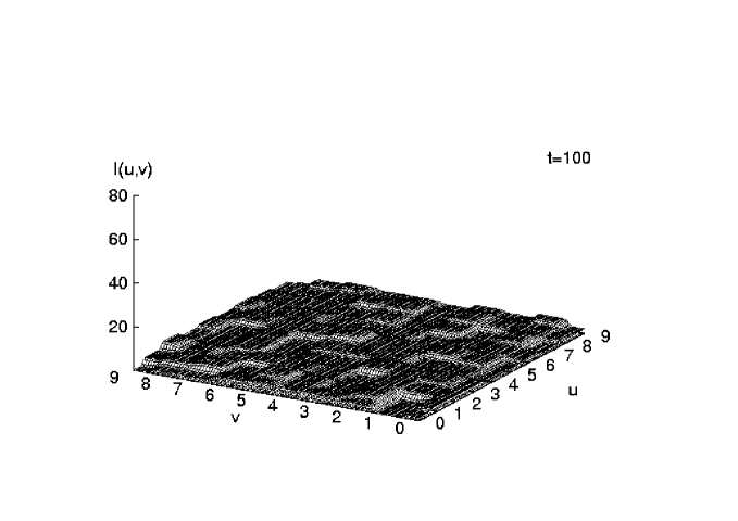
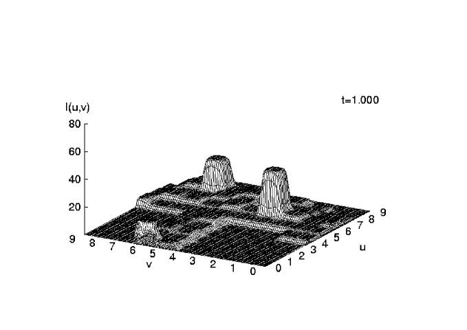
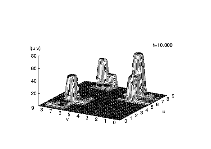
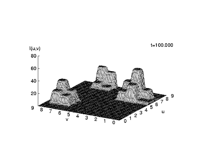
Figure 3: Spatial density of employed agents, $l(u,v)$, for different times $t$ (for the parameters and initial conditions of the simulation, see text).

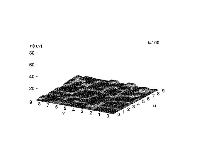
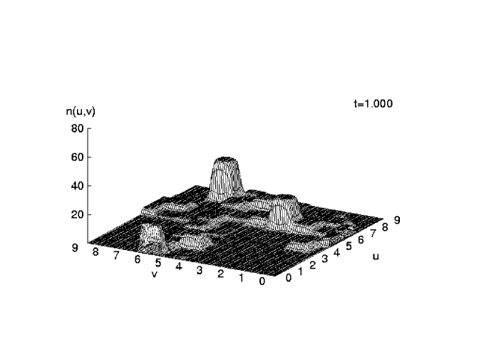
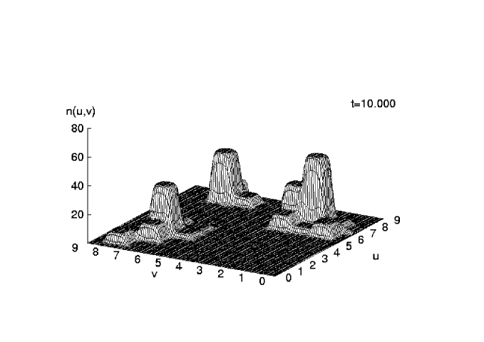
Figure 4: Spatial density of unemployed agents, $n(u,v)$, for different times $t$ (for the parameters and initial conditions of the simulation, see text).

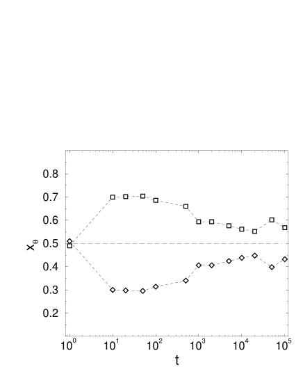
Figure 5: Total share $x_{\theta}$ of employed agents ($\Box$) and unemployed agents ($\Diamond$) vs. time $t$. The marks indicate simulation data which correspond to Figs. 3, 4.

The simulation shows that the evolution of the densities occurs on two stages:

(i) During the first stage (for $t<1.000$) we have a significant higher share of employed agents (up to 70 percent of the agents community). They are broadly distributed in numerous small economic centers, which have an employment density of about 5. This can be understood using Figs. 1, 2. The increase of the output due to cooperative effects allows the fast establishment of numerous small firms, which count on the mutual stimulations among their workers and in the beginning offer higher wages (compared to the model without cooperative effects).

This growth strategy, however, is not sufficient for output on larger scales, because the marginal product drastically decreases (before it may increase again for an above critical employment density). As a result the wages may fall (possibly below the minimum wage rate, $\omega^{\star}$), which prevents further growth. So, the first stage is characterized by the coexistence of numerous small economic centers.

(ii) During the second and much longer stage (for $t>1.000$), some of these small centers overcome this economic bottleneck, which allows them to grow further. In the simulations, this crossover occured between $t=500$ and $t=800$. In the model considered here, we have only one variable input, labor, so the crossover is mainly due to stochastic fluctuations in $l(r,t)$.

After the bottleneck, the marginal output increases again, and also the wage increases with the density of employment (cf. Figs. 1, 2). This in turn effects the migration of the unemployed agents, which, due to eq. (2), is determined by two forces: the local attraction to areas with higher wages, and the stochastic influences which keep them moving. With $\partial\omega/\partial l>0$, the attraction may exceed the stochastic forces, so the unemployed agents are bound to these regions, once they got there. This, in turn is important for the further growth of these economic centers, which needs agents to hire. As a result, we observe on the spatial level the concentration of employed and unemployed agents in the same regions.

For their further growth, the economic centers which overcome the bottleneck, locally attract the labor force at the expense of the former small economic centers. As a result of the competition process, these small centers, which previously employed about 70 percent of the agents, dissapear. In the new (larger) centers however, only 60 percent of the agents can be employed (cf. Fig. 5), so the competition and the resulting large-scale production effectively results also in an increase of unemployment. But the employment rate of 60 percent seems to be a stable value for the given parameter setup, since it is kept also in the long run, with certain fluctuations.

The concentration process described above, leads to the existence of different extended major economic regions, shown in Figs. 3, 4, which each consist of some subregions (in terms of boxes). In the long run (up to t=100.000) we find some remarkable features of the dynamics:

• a stable coexistence of the major economic regions, which keep a certain distance from each other. This critical distance - which is a self-organized phenomenon - prevents the regions from detracting each other. In fact, finally there is no force between these regions which would pull off the employed or unemployed agents and guide them over long distances to other regions. Thus, the coexistence is really a stable one.

• a quasi-stationary non-equilibrium within the major economic centers. As we see, even in the long run, the local densities of employed and unemployed agents do not reach a fixed stationary value. Within the major regions, there are still exchange processes between the participating boxes, hiring and firing, attraction and migration. Hence, the total share of employed agents continues to fluctuate around the mean value of 60 percent (cf. Fig. 5).

6 Conclusions

In this paper, we have proposed a simple dynamic model to descibe migration and economic aggregation within the framework of Active Brownian particles. We consider two types of particles (or agents); employed agents, which are immobile, but (as the result of their work) generate a wage field, and the unemployed agents which migrate by responding to local gradients in the wage field. Further a transition between employed and unemployed agents (hiring and firing) is considered.

The economic assumptions to be used in the model, are concluded in only three functions: (a) the derivative $\partial\omega/\partial l$, which describes how the local wage depends on the employment density, (b) $k^{+}$, (c) $k^{-}$, which are the hiring and firing rates. These functions can be determined using a production function, $Y(l)$, which describes the output of production dependent on the variable input of labor. Our ansatz for $Y(l)$ specifically counts on the influence of cooperative interactions between the agents on a certain scale of production.

As the result of our dynamic model, we find the establishment of distinct economic centers out of a random initial distribution. The evolution of these centers occurs in two different stages. During the first stage, small economic centers are formed based on the positive feedback of mutual stimulation/cooperation among the agents. During the second and much longer stage, some of these small centers grow at the expense of others, which leads to the interesting situation that in our model economic growth and decline occur at the same time, but at different locations, which results in specific spatial-temporal patterns. The competition finally leads to the concentration of the labor force in different extended economic regions. This crossover to large-scale production is accompanied by an increase in the unemployment rate.

Although the extended economic regions are in an internal, quasistationary non-equilibrium, we observe the stable coexistence between these regions. This is an important result, which agrees e.g. with the central place theory of economics (Christaller, 1933, Lösch, 1940). Different from an attempt by Krugman (1992), who also focused on this problem, we find that (i) the coexistence is stable, even at the presence of fluctuations, (ii) the centers not necessarily have to have the same number of employed agents, to coexist, (iii) the dynamics does not simply converges into an equilibrium state, but the centers exist in an quasistationary non-equilibrium state and still follow a stochastic eigendynamics.

One question, which will be tackled in a forthcoming paper, is about the influence of the different parameters. We have seen in the simulations, that cooperative effects are able to initiate an increase in the economic output, which leads to the establishment of many small firms. But the final situation does not include any of those small firms and seems to be independent of this intermediate state. This is mainly due to the fact, that we considered only one product. A more complex production function with different outputs, however, should also result in the coexistence of small (innovative) firms and large scale production.

Another important issue is to understand the relation between the response of the agents to local gradients in the wage field, on one hand, and stochastic influences, on the other hand. Most likely, there exist critical parameters which may describe a “phase transition” within the agents behavior, which eventually results in different types of spatial-temporal coexistence.

Finally, one may argue that the simple model proposed here, is not the simplest one to describe the economic aggregation. Hence, the minimalistic agents discussed in Sect. 1, could be even more minimalistic. One example is the response of the employed agents to gradients in the wage field, expressed in the parameter $q$ which enters the firing rate, $k^{-}$. $q=0$ simply means that internal reasons are neglected, and the agent is fired only due to external reasons. This might be also a reasonable assumption, however, it includes a pitfall. In a growing economy, eventually almost all unemployed agents might be hired at some locations. But, as long as $dY/dl>\omega^{\star}$, employed agents are almost never fired, thus there is a shortage of free agents for further growth. Eventually the dynamics sticks in a dead-lock situation, because agents cannot move even if there are locations in their neighborhood which may offer them a higher wage. Therefore, it is reasonable to choose $q>0$, but it is important to understand the role of $q$, for instance, for the final patterns observed.

So, we conclude that our model may serve as a toy model for simulating the influence of different social and economic assumptions on the spatial-temporal patterns in migration and economic aggregation.

References

Anderson, P.W., Arrow, K.J., Pines, D. (eds.) (1988). The Economy as an Evolving Complex System, Reading, MA: Addison Wesley.

Arthur, W. B. (1993). On Designing Economic Agents that Behave Like Human Agents, Journal of Evolutionary Economics 3, 1–22.

Arthur, W. B.; Durlauf, S. N.; Lane, D. (eds.) (1997). The Economy as an Evolving Complex System II, Reading, MA: Addison Wesley.

Ben-Jacob, E.; Cohen, I., Czirók, A. (1995). Smart bacterial colonies: From complex patterns to cooperative evolution, Fractals 3, 849-868.

Case, K.E.; Fair, R.C. (1992). Principles of Economics, Englewood Cliffs: Prentice-Hall.

Christaller, W. (1933). Central Places in Southern Germany, Jena: Fischer (English translation by C.W. Baskin, London: Prentice Hall, 1966).

Dendrinos, D.; Haag, G. (1984). Towards a stochastic theory of location: Empirical evidence, Geogr. Anal. 16, 287-300.

Ebeling, W.; Schweitzer, F.; Tilch, B. (1998). Active Brownian Particles with Energy Depots Modelling Animal Mobility, BioSystems (in press).

Epstein, J. M.; Axtell, R. (1996). Growing Artificial Societies: Social Science from the Bottom Up, Cambridge, MA: MIT Press/Brookings.

Feistel, R., Ebeling, W. (1989). Evolution of Complex Systems. Self-Organization, Entropy and Development, Dordrecht: Kluwer.

Fujita, M. (1989). Urban Economic Theory, Cambridge: Cambridge University Press.

Haag, G. (1994). The Rank-Size Distribution of Settlements as a Dynamic Multifractal Phenomenon, Chaos, Solitons & Fractals 4, 519-534.

Haag, G.; Munz, M.; Pumain, P.; Sanders, L.; Saint-Julien, Th. (1992). Interurban migration and the dynamics of a system of cities: 1. The stochastic framework with an application to the French urban system, Environment and Planning A 24, 181-198.

Helbing, D.; Schweitzer, F.; Keltsch, J.; Molnár, P. (1997). Active Walker Model for the Formation of Human and Animal Trail Systems, Physical Review E 56/3, 2527-2539.

Henderson, J.V. (1988). Urban Development. Theory, Fact, and Illusion, Oxford: Oxford University press.

Holland, J.; Miller, J. (1991). Adaptive Agents in Economic Theory, American Economic Review Papers and Proceedings 81, 365–370.

Kirman, A. (1993). Ants, Rationality, and Recruitment, The Quarterly Journal of Economics, 108, 37-155.

Krugman, P. (1991). Increasing returns and economic geography, Journal of Political Economy 99, 483–499.

Krugman, P. (1992). A dynamic spatial model, National Bureau of Economic Resarch Working Paper No. 4219.

Krugman, P. (1996 a). Urban Concentration: The role of increasing returns and transportation costs, Intern. Regional Science Review 19, 5-30.

Krugman, P. (1996 b). The Self-Organizing Economy, Oxford: Blackwell.

Lam, L. (1995). Active Walker Models for Complex Systems, Chaos, Solitons & Fractals 6, 267-285.

Lam, L.; Pochy, R. (1993). Active-Walker Models: Growth and Form in Nonequilibrium Systems, Computers in Physics 7, 534-541.

Lane, D. (1992). Artificial Worlds and Economics, Journal of Evolutionary Economics 3, 89–107.

Lösch, A. (1940). The Economics of Location, Jena: Fischer (English translation, New Haven: Yale University Press, 1954).

Maes, P. (ed.) (1990). Designing Autonomous Agents. Theory and Practice From Biology to Engineering and Back, Cambridge, MA: MIT Press.

Marimon, R.; McGrattan, E.; Sargent, T. J. (1990). Money as a Medium of Exchange in an Economy with Artificially Intelligent Agents, Journal of Economic Dynamics and Control 14, 329–373.

Müller, J. P.; Wooldridge, M. J.; Jennings, N. R. (eds.) (1997). Intelligent agents III : agent theories, architectures, and languages, Berlin: Springer.

Puu, T. (1993). Pattern formation in spatial economics, Chaos, Solitons & Fractals 3, 99-129.

Schimansky-Geier, L.; Mieth, M.; Rose, H.; Malchow, H. (1995). Structure Formation by Active Brownian Particles, Physics Letters A 207, 140.

Schimansky-Geier, L.; Schweitzer, F.; Mieth, M. (1997). Interactive Structure Formation with Brownian Particles, in: F. Schweitzer (ed.): Self-Organization of Complex Structures: From Individual to Collective Dynamics, London: Gordon and Breach, pp. 101-118.

Schweitzer, F. (1997). Active Brownian Particles: Artificial Agents in Physics, in: L. Schimansky-Geier, T. Pöschel (eds.): Stochastic Dynamics, Berlin: Springer, pp. 358-371.

Schweitzer, F.; Lao, K.; Family, F. (1997). Active Random Walkers Simulate Trunk Trail Formation by Ants, BioSystems 41, 153-166.

Schweitzer, F.; Schimansky-Geier, L. (1994). Clustering of Active Walkers in a Two-Component System, Physica A 206, 359-379.

Schweitzer, F.; Silverberg, G. (eds.) (1998). Evolution and Self-Organization in Economics, Berlin: Duncker & Humblot.

Schweitzer, F.; Steinbrink, J. (1997). Urban Cluster Growth: Analysis and Computer Simulation of Urban Aggregations, in: F. Schweitzer (ed.), Self-Organization of Complex Structures: From Individual to Collective Dynamics, London: Gordon and Breach, pp. 501-518.

Silverberg, G. (1997). Is there Evolution after Economics?, in: F. Schweitzer (ed.): Self-Organization of Complex Structures: From Individual to Collective Dynamics, London: Gordon and Breach, pp. 415-425.

Silverberg, G.; Verspagen, B. (1994). Collective Learning, Innovation and Growth in a Boundedly Rational, Evolutionary World, Journal of Evolutionary Economics 4, 207-226.

Steels, L. (ed.) (1995). The biology and technology of intelligent autonomous agents, Berlin: Springer.

Steuernagel, O., Ebeling, W., Calenbuhr, V. (1994). An Elementary Model for Directed Active Motion, Chaos, Solitons & Fractals 4, 1917-1930.

Wei-Bin, Z. (1991). Synergetic Economics, New York: Springer.

Weidlich, W. (1991). Physics and Social Science – The Approach of Synergetics, Physics Reports 204, 1-163.

Weidlich, W. (1997). From Fast to Slow Processes in the Evolution of Urban and Regional Settlement Structures, in: F. Schweitzer (ed.): Self-Organization of Complex Structures: From Individual to Collective Dynamics, London: Gordon and Breach, pp. 475-488.

Weidlich, W.; Munz, M. (1990 a). Settlement formation, I. A dynamic theory; Annals of Regional Science 24, 83-106.

Weidlich, W.; Munz, M. (1990 b). Settlement formation, II. Numerical simulation; Annals of Regional Science 24, 177-196.