Modelling Collective Opinion Formation by Means of Active Brownian Particles

Abstract

The concept of active Brownian particles is used to model a collective opinion formation process. It is assumed that individuals in community create a two-component communication field that influences the change of opinions of other persons and/or can induce their migration. The communication field is described by a reaction-diffusion equation, the opinion change of the individuals is given by a master equation, while the migration is described by a set of Langevin equations, coupled by the communication field. In the mean-field limit holding for fast communication we derive a critical population size, above which the community separates into a majority and a minority with opposite opinions. The existence of external support (e.g. from mass media) changes the ratio between minority and majority, until above a critical external support the supported subpopulation exists always as a majority. Spatial effects lead to two critical “social” temperatures, between which the community exists in a metastable state, thus fluctuations below a certain critical wave number may result in a spatial opinion separation. The range of metastability is particularly determined by a parameter characterizing the individual response to the communication field. In our discussion, we draw analogies to phase transitions in physical systems.

1 Introduction

In recent years, there has been a lot of interest in applications of physical paradigms to a quantitative description of social weidl-haag-83 ; galam-90 ; weidl-91 ; galam-91 ; valla-nowak-94 ; gilbert-doran-94 ; helbing-95 and economic processes stanley96 ; laherrere-sornette98 ; challet-zhang98 ; mantegna-stanley99

Methods of synergetics haken-78 ; wei-bin-91 , stochastic processes helbing-93 ; bouchaud-sornette94 , deterministic chaos dendrinos-sonis-90 ; lorenz-93 ; holyst-hagel-haa-weidl-96 ; holyst-hagel-haag-97 and lattice gas models lewenst-nowak-latane-92 ; kacp-holyst-96 ; galam97 have been successfully applied for this purpose.

The formation of public opinion nowak-szam-latane-90 ; schw-bart-pohlm-91 ; galam-moscovich-91 ; latane-nowak-liu-94 ; kacp-holyst-97 ; plewczynski98 ; kacp-holyst99 is among the challenging problems in social science, because it reveals a complex dynamics, which may depend on different internal and external influences. We mention the influence of political leaders, the biasing effect of mass media, as well as individual features, such as persuasion or support for other opinions.

A quantitative approach to the dynamics of opinion formation is given by the concept of social impact lewenst-nowak-latane-92 ; nowak-szam-latane-90 , which is based on methods similar to the cellular automata approach wolfram-86 ; galam97 . The social impact describes the force on an individual to keep or to change its current opinion. A short outline of this model is given in Sect. 2. The equilibrium statistical mechanics of the social impact model was formulated in lewenst-nowak-latane-92 , while in kacp-holyst-96 ; kacp-holyst-97 ; kacp-holyst99 the occurrence of phase transitions and bistability in the presence of a strong leader or an external impact have been analysed.

Despite these extensive studies of the social impact model, there are several basic disadvantages of the concept. In particular, the social impact theory assumes, that the impact on an individual is updated with infinite velocity, and no memory effects are considered. Further, there is no migration of the individuals, and any “spatial” distribution of opinions refer to a “social”, but not to the physical space.

In fact, the model of social impact has not been developed to describe processes of opinion diffusion and migration. In this paper, we present an alternative approach to the social impact model of collective opinion formation, which tries to include these features. Our model is based on active Brownian particles, which interact via a communication field. This field considers the spatial distribution of the individual opinions, further, it has a certain life time, reflecting a collective memory effect and it can spread out in the community, modeling the transfer of information.

Active Brownian particles lsg-mieth-rose-malch-95 ; lsg-schw-mieth-97 ; schw-agent-97 are Brownian particles with the ability to take up energy from the environment, to store it in an internal depot fs-eb-tilch-98-let ; eb-fs-tilch-98 and to convert internal energy to perform different activities, such as metabolism, motion, change of the environment, or signal-response behavior. As a specific action, the active Brownian particles (or active walkers, within a discrete approximation) are able to generate a self-consistent field, which in turn influences their further movement and physical or chemical behavior. This non-linear feedback between the particles and the field generated by themselves results in an interactive structure formation process on the macroscopic level. Hence, these models have been used to simulate a broad variety of pattern formation processes in complex systems, ranging from physical to biological and social systems lam-po-93 ; schwei-lsg-94 ; lam-95 ; schwei-lao-fam-97 ; helb-schw-et-97 ; fs-98 .

In Sect. 2, we specify the model of active Brownian particles for the formation of collective opinion structures. In Sect. 3, we discuss the limiting case of fast communication between the individuals. Further, we investigate the influence of an external support and derive critical parameters for the existence of subpopulations as majorities or minorities. In Sect. 4, we investigate spatial opinion structures, and estimate critical wave numbers for the fluctuations, which lead to a spatial separation of the opinions. By deriving two different critical temperatures, we draw an analogy to the theory of phase transitions.

2 Stochastic Model of Opinion Change and Migration

Let us consider a 2-dimensional spatial system with the total area $A$, where a community of $N$ individuals (members of a social group) exists. Each of them can share one of two opposite opinions on a given subject, denoted as $\theta_{i}=\pm 1;i=1,...,N$. Here, $\theta_{i}$ is considered as an individual parameter, representing an internal degree of freedom. Within a stochastic approach, the probability $p_{i}(\theta_{i},t)$ to find the individual $i$ with the opinion $\theta_{i}$, changes in the course of time due to the following master equation:

$$\frac{d}{dt}p_{i}(\theta_{i},t)=\sum_{\theta_{i}^{\prime}}w(\theta_{i}|\theta_{i}^{\prime})p_{i}(\theta_{i}^{\prime},t)-p_{i}(\theta_{i},t)\sum_{\theta_{i}^{\prime}}w(\theta_{i}^{\prime}|\theta_{i}).$$ (1)

Here, $w(\theta_{i}^{\prime}|\theta_{i})$ means the transition rate to change the opinion $\theta_{i}$ into one of the possible opinions $\theta_{i}^{\prime}$ during the next time step, with $w(\theta_{i}|\theta_{i})=0$. In the considered case, there are only two possibilities, either $\theta_{i}=+1\to\theta_{i}^{\prime}=-1$, or $\theta_{i}=-1\to\theta_{i}^{\prime}=+1$. In the social impact theory lewenst-nowak-latane-92 ; nowak-szam-latane-90 , it is assumed that the change of opinions depends on the social impact, $I_{i}$, and a “social temperature”, $T$ kacp-holyst-96 ; kacp-holyst-97 . A possible ansatz for the transition rate reads:

$$w(\theta_{i}^{\prime}|\theta_{i})=\eta\,\exp\{I_{i}/T\}.$$ (2)

Here, $\eta$ [1/s] defines the time scale of the transitions. $T$ represents the erratic circumstances of the opinion change: in the limit $T\to 0$ the opinion change is more determined by $I_{i}$, leading to deterministic transitions. As eq. (2) indicates, the likelyhood for changing the opinion is rather small, if $I_{i}<0$. Hence, a negative social impact on individual $i$ represents a condition for stability. To be specific, in the social impact theory, $I_{i}$ may consist of three parts:

$$I_{i}=I^{p}_{i}+I^{s}_{i}+I^{ex}_{i}$$ (3)

$I^{p}_{i}$ represents influences imposed on the individual by other members of the group, e.g. to change or to keep its opinion. $I^{s}_{i}$, on the other hand, is kind of a self-support for the own opinion, $I^{s}_{i}<0$, and $I^{ex}_{i}$ represents external influences, e.g. from government policy, mass media, etc. which may also support a certain opinion.

Within a simplified approach of the social impact theory, every individual can be ascribed a single parameter, the “strength”, $s_{i}$. Furthermore, a social distance $d_{ij}$ is defined, which measures the distance between each two individuals $(i,j)$ in a social space lewenst-nowak-latane-92 ; nowak-szam-latane-90 , which does not necessarily coincide with the physical space. It is assumed that the impact between two individuals decreases with the social distance in a non-linear manner. The above assumptions are included in the following ansatz kacp-holyst-96 ; kacp-holyst-97 :

$$I_{i}=-\theta_{i}\sum_{j=1,j\neq i}^{N}s_{j}\theta_{j}/d_{ij}^{n}\;-\varepsilon s_{i}\;+e_{i}\theta_{i}$$ (4)

$\varepsilon$ is the so-called self-support parameter, and $n>0$ is a model constant. The external influence, $e_{i}$ may be regarded as a global preference towards one of the opinions. A negative social impact on individual $i$ is obtained, (i) if most of the opinions in its social vicinity match its own opinion, or (ii) if the impact resulting from opposite opinions is at least not large enough to compensate its self-support, or (iii) if the external influences do not force the individual to change its opinion, regardless of self-support or the impact of the community.

In the form outlined above, the concept of social impact has certain drawbacks: The social impact theory assumes that the impact on an individual is instantaneously updated, if some opinions are changed in the group (which basically means a communication with infinite velocity). Spatial effects in a physical space are not considered here, any “spatial” distribution of opinions refers to the social space. Moreover, the individuals are not allowed to move. Finally, no memory effects are considered in the social impact, the community is only affected by the current state of the opinion distribution, regardless of its history and past experience.

In this paper, we want to modify the theory by including some important features of social systems: (i) the existence of a memory, which reflects the past experience, (ii) an exchange of information in the community with a finite velocity, (iii) the influence of spatial distances between individuals, (iv) the possibility of spatial migration for the individuals. It seems more realistic to us that individuals have the chance to migrate to places where their opinion is supported rather than change their opinion. And in most cases, individuals are not instantaneously affected by the opinions of others, especially if they are not in their close vicinity.

As a basic element of our theory, a scalar spatio-temporal communication field $h_{\theta}(\mbox{\boldmath$r$},t)$ is used. Every individual contributes permanently to this field with its opinion $\theta_{i}$ and with its personal strength $s_{i}$ at its current spatial location $\mbox{\boldmath$r$}_{i}$. The information generated this way has a certain life time $1/\beta$ [s], further it can spread throughout the system by a diffusion-like process, where $D_{h}$ [m²/s] represents the diffusion constant for information exchange. We have to take into account that there are two different opinions in the system, hence the communication field should also consist of two components, $\theta=\{-1,+1\}$, each representing one opinion. For simplicity, it is assumed that the information resulting from the different opinions has the same life time and the same way of spatial distribution; more complex cases can be considered as well.

The spatio-temporal change of the communication field can be summarized in the following equation:

$$\frac{\partial}{\partial t}h_{\theta}(\mbox{\boldmath$r$},t) = \sum_{i=1}^{N}s_{i}\;\delta_{\theta,\theta_{i}}\;\delta(\mbox{\boldmath$r$}-\mbox{\boldmath$r$}_{i})\;$$ (5)

$$-\;\beta h_{\theta}(\mbox{\boldmath$r$},t)\;+\;D_{h}\Delta h_{\theta}(\mbox{\boldmath$r$},t).$$

Here, $\delta_{\theta,\theta_{i}}$ is the Kronecker Delta indicating that the individuals contribute only to the field component which matches their opinion $\theta_{i}$. $\delta(\mbox{\boldmath$r$}-\mbox{\boldmath$r$}_{i})$ means Dirac’s Delta function used for continuous variables, which indicates that the individuals contribute to the field only at their current position, $\mbox{\boldmath$r$}_{i}$. We note that this equation is a stochastic partial differential equation with

$$n^{micr}(\mbox{\boldmath$r$},t)=\sum_{i=1}^{N}\delta(\mbox{\boldmath$r$}-\mbox{\boldmath$r$}_{i})$$ (6)

being the microscopic density lsg-schw-mieth-97 of the individuals changing their position due to Eq. (8). Hence, the changes of the communication field $h_{\theta}(\mbox{\boldmath$r$},t)$ are measured in units of a density of the personal strength $s_{i}$.

Instead of a social impact, the communication field $h_{\theta}(\mbox{\boldmath$r$},t)$ influences the individual $i$ as follows: At a certain location $\mbox{\boldmath$r$}_{i}$, the individual with opinion $\theta_{i}=+1$ is affected by two kinds of information: the information resulting from individuals who share his/her opinion, $h_{\theta=+1}(\mbox{\boldmath$r$}_{i},t)$, and the information resulting from the opponents $h_{\theta=-1}(\mbox{\boldmath$r$}_{i},t)$. The diffusion constant $D_{h}$ determines how fast he/she will receive any information, and the decay rate $\beta$ determines, how long a generated information will exist. Dependent on the local information, the individual has two opportunities to act: (i) it can change its opinion, (ii) it can migrate towards locations which provide a larger support of its current opinion. These opportunities are specified in the following.

For the change of opinions, we can adopt the transition probability, Eq. (2), by replacing the influence of the social impact $I_{i}$ with the influence of the local communication field. A possible ansatz reads:

$$w(\theta_{i}^{\prime}|\theta_{i}) = \eta\,\exp\{[h_{\theta^{\prime}}(\mbox{\boldmath$r$}_{i},t)-h_{\theta}(\mbox{\boldmath$r$}_{i},t)]/T\}$$

$$w(\theta_{i}|\theta_{i}) = 0$$ (7)

As in Eq. (2), the probability to change opinion $\theta_{i}$ is rather small, if the local field $h_{\theta}(\mbox{\boldmath$r$}_{i},t)$, which is related to the support of opinion $\theta_{i}$, overcomes the local influence of the opposite opinion. This effect, however, is scaled again by the social temperature $T$, which is a measure for the randomness in social interaction. Note, that the social temperature is measured in units of the communication field.

The movement of the individual located at space coordinate $\mbox{\boldmath$r$}_{i}$ may depend both on erratic circumstances and on the influence of the communication field. Within a stochastic approach, this movement can be described by the following overdamped Langevin equation:

$$\frac{d\mbox{\boldmath$r$}_{i}}{dt}=\alpha_{i}\left.\frac{\partial h_{e}(\mbox{\boldmath$r$},t)}{\partial r}\right|_{\mbox{\boldmath$r$}_{i}}+\sqrt{2\,D_{n}}\;\xi(t).$$ (8)

In the last term of Eq. (8) $D_{n}$ means the spatial diffusion coefficient of the individuals. The random influences on the movement are modeled by a stochastic force with a $\delta$-correlated time dependence, i.e. $\xi(t)$ is the white noise with $\left\langle\xi_{i}(t)\,\xi_{j}(t^{\prime})\right\rangle=\delta_{ij}\,\delta(t-t^{\prime})$.

The term $h_{e}(\mbox{\boldmath$r$},t)$ in Eq. (8) means an effective communication field which results from $h_{\theta}(\mbox{\boldmath$r$},t)$ as specified below. It follows that the overdamped Langevin Eq. (8) considers the response of the individual to the gradient of the field $h_{e}(\mbox{\boldmath$r$},t)$, where $\alpha_{i}$ is the individual response parameter, weighting the importance of the information received. In the considered case, the effective communication field $h_{e}(\mbox{\boldmath$r$},t)$ is a certain function of both components, $h_{\pm 1}(\mbox{\boldmath$r$},t)$, of the communication field, see Eq. (5). One can consider different types of response, for example the following:

1. The individuals try to move towards locations which provide the most support for their current opinion $\theta_{i}$. In this case, they only count on the information which matches their opinion, $h_{e}(\mbox{\boldmath$r$},t)=h_{\theta}(\mbox{\boldmath$r$},t)$, and follow the local ascent of the field $(\alpha_{i}>0)$.

2. The individuals try to move away from locations which provide any negative pressure on their current opinion $\theta_{i}$. In this case, they count on the information resulting from opposite opinions $(\theta^{\prime})$, $h_{e}(\mbox{\boldmath$r$},t)=h_{\theta^{\prime}}(\mbox{\boldmath$r$},t)$, and follow the local descent of the field $(\alpha_{i}<0)$.

3. The individuals try to move away from locations, if they are forced to change their current opinion $\theta_{i}$, but they can accept a vicinity of opposite opinions, as long as these are not dominating. In this case, they count on the information resulting from both supporting and opposite opinions, and the local difference between them is important: $h_{e}(\mbox{\boldmath$r$},t)=[h_{\theta}(\mbox{\boldmath$r$},t)-h_{\theta^{\prime}}(\mbox{\boldmath$r$},t)]$ with $\alpha_{i}>0$.

Additionally, the response parameter can also consider that the response occurs only, if the absolute value of the effective field is locally above a certain threshold $h_{thr}$: $\alpha_{i}=\Theta\left[\left|h_{e}(\mbox{\boldmath$r$},t)\right|-h_{thr}\right]$, with $\Theta[y]$ being the Heavyside function: $\Theta=1$, if $y>0$, otherwise $\Theta=0$. We note that for the further discussions in Sect. 3 and 4, we assume $h_{e}(\mbox{\boldmath$r$},t)=h_{\theta}(\mbox{\boldmath$r$},t)$ for the effective communication field (case i), while $\alpha_{i}\equiv\alpha$ is treated as a positive constant independent of $i$ and $h_{e}(\mbox{\boldmath$r$},t)$.

In order to summarize our model, we note the non-linear feedback between the individuals and the communication field as shown in Fig. 1. The individuals generate the field, which in turn influences their further movement and their opinion change. In terms of synergetics, the field plays the role of an order parameter, which couples the individual actions, and this way initiates spatial structures and coherent behavior within the social group.

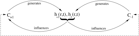
Figure 1: Circular causation between the individuals with different opinions, $C_{-1}$, $C_{+1}$ and the two-component communication field, $h_{\theta}(\mbox{\boldmath$r$},t)$.

The complete dynamics of the community can be formulated in terms of the canonical $N$-particle distribution function

$$P(\underline{\theta},\underline{r},t)=P(\theta_{1},\mbox{\boldmath$r$}_{1},...,\theta_{N},\mbox{\boldmath$r$}_{N},t),$$ (9)

which gives the probability to find the $N$ individuals with the opinions $\theta_{1},...,\theta_{N}$ in the vicinity of $\mbox{\boldmath$r$}_{1},....,\mbox{\boldmath$r$}_{N}$ on the surface $A$ at time $t$. Considering both opinion changes and movement of the individuals, the master equation for $P(\underline{\theta},\underline{r},t)$ reads:

$$\frac{\displaystyle\partial}{\displaystyle\partial t}P(\underline{\theta},\underline{r},t)=\sum_{\underline{\theta^{\prime}}\neq\underline{\theta}}\Big{[}w(\underline{\theta}|\underline{\theta}^{\prime})P(\underline{\theta}^{\prime},\underline{r},t)-w(\underline{\theta}^{\prime}|\underline{\theta})P(\underline{\theta},\underline{r},t)\Big{]}$$

$$-\sum_{i=1}^{N}\Big{[}\nabla_{i}\,\left(\alpha\,\nabla_{i}h_{\theta}(\mbox{\boldmath$r$},t)\,P(\underline{\theta},\underline{r},t)\right)-D_{n}\,\Delta_{i}P(\underline{r},\underline{\theta},t)\Big{]}$$

(10)

The first line of the right-hand side of Eq. (10) describes the “gain” and “loss” of individuals (with the coordinates $\mbox{\boldmath$r$}_{1},...,\mbox{\boldmath$r$}_{N}$) due to opinion changes, where $w(\underline{\theta}|\underline{\theta}^{\prime})$ means any possible transition within the opinion distribution $\underline{\theta}^{\prime}$ which leads to the assumed distribution $\underline{\theta}$. The second line describes the change of the probability density due to the motion of the individuals on the surface. Eq. (10) together with eqs. (5), (7) forms a complete description of our system.

3 The Case of Fast Communication

3.1 Derivation of Mean Value Equations

Let us first restrict to the case of very fast exchange of information in the system. Then, spatial inhomogenities are equalized immediately, hence, the communication field $h_{\theta}(\mbox{\boldmath$r$},t)$ can be approximated by a mean field $\bar{h}_{\theta}(t)$:

$$\bar{h}_{\theta}(t)=\frac{1}{A}\int\limits_{A}h_{\theta}(\mbox{\boldmath$r$},t)\;dr^{2},$$ (11)

where $A$ means the system size. The equation for the mean field $\bar{h}_{\theta}(t)$ results from eq. (5):

$$\frac{\partial\bar{h}_{\theta}(t)}{\partial t}=-\beta\bar{h}_{\theta}(t)+s\bar{n}_{\theta}$$ (12)

with $s_{i}\equiv s$ and the mean density

$$\bar{n}_{\theta}=\frac{N_{\theta}}{A}\;\;;\;\;\;\bar{n}=\frac{N}{A},$$ (13)

where the number of individuals with a given opinion $\theta$ fulfils the condition

$$\sum_{\theta}N_{\theta}=N_{+1}+N_{-1}=N={\rm const.}$$ (14)

We note that in the mean–field approximation no spatial gradients in the communication field exist. Hence, there is no additional driving force for the individuals to move, as assumed in Eq. (8). Such a situation can be imagined for communities existing in very small systems with small distances between different groups. In particular, in such small communities also the assumption of a fast information exchange holds. Thus, in this section, we restrict our discussion to subpopulations with a certain opinion rather than to individuals at particular locations.

Let $p(N_{\theta},t)$ denote the probability to find $N_{\theta}$ individuals in the community which shares opinion $\theta$. The master equation for $p(N_{+1},t)$ explicitely reads:

$$\frac{\partial}{\partial t}p(N_{+1},t) = W(N_{+1}|N_{+1}-1)\,p(N_{+1}-1,t)$$ (15)

$$+W(N_{+1}|N_{+1}+1)\,p(N_{+1}+1,t)$$

$$-p(N_{+1},t)\left[W(N_{+1}+1|N_{+1})\right.$$

$$+\left.W(N_{+1}-1|N_{+1})\right].$$

The transition rates $W(M|N)$ appearing in Eq. (15) are assumed to be proportional to the probability to change a given opinion, eq. (7), and to the number of individuals which can change their opinion into the given direction:

$$W(N_{+1}+1|N_{+1}) = N_{-1}\,\eta\,\exp{\{(\bar{h}_{+1}-\bar{h}_{-1})/T\}},$$ (16)

$$W(N_{+1}-1|N_{+1}) = N_{+1}\,\eta\,\exp{\{-(\bar{h}_{+1}-\bar{h}_{-1})/T\}}.$$

The mean values for the number of individuals with a certain opinion can be derived from the master equation (15)

$$\langle N_{\theta}(t)\rangle=\sum_{\{N_{\theta}\}}N_{\theta}\;p(N_{\theta},t),$$ (17)

where the summation is over all possible numbers of $N_{\theta}$ which obey the condition eq. (14). From eq. (17), the deterministic equation for the change of $\left\langle N_{\theta}\right\rangle$ can be derived in the first approximation as follows schw-lsg-eb-ulb (see also weidl-haag-83 ; weidl-91 ; helbing-95 ):

$$\frac{d}{dt}\left\langle N_{\theta}\right\rangle=\left\langle W(N_{\theta}+1|N_{\theta})-W(N_{\theta}-1|N_{\theta})\right\rangle$$ (18)

For $N_{+1}$, this equation reads explicitely:

$$\frac{d}{dt}\left\langle N_{+1}\right\rangle = \left\langle N_{-1}\,\eta\,\exp\left[\frac{\bar{h}_{+1}(t)-\bar{h}_{-1}(t)}{T}\right]\right.$$ (19)

$$\left.-N_{+1}\,\eta\,\exp\left[-\frac{\bar{h}_{+1}(t)-\bar{h}_{-1}(t)}{T}\right]\right\rangle$$

Introducing now the fraction of a subpopulation with opinion $\theta$, $x_{\theta}=\langle N_{\theta}\rangle/N$, and using the standard approximation to factorize eq. (19), we can write it as:

$$\dot{x}_{+1} = (1-x_{+1})\,\eta\,\exp(a)-x_{+1}\,\eta\,\exp(-a),$$ (20)

$$a = \left[\bar{h}_{+1}(t)-\bar{h}_{-1}(t)\right]/T.$$

Via $\Delta\bar{h}(t)=\bar{h}_{+1}-\bar{h}_{-1}$, this equation is coupled with the equation

$$\Delta\dot{\bar{h}}=-\beta\,\Delta\bar{h}+s\bar{n}\Big{(}2x_{+1}-1\Big{)}$$ (21)

which results from eq. (12) for the two field components.

3.2 Critical and Stable Subpopulation Sizes

Within a quasistationary approximation, we can assume that the communication field relaxes faster than the distribution of the opinions into a stationary state. Hence, with $\dot{\bar{h}}_{\theta}=0$, we find from Eq. (12):

$$\begin{array}[]{lcl}\bar{h}_{+1}^{stat}=\frac{\displaystyle s\,\bar{n}}{\displaystyle\beta}x_{+1}&;&\bar{h}_{-1}^{stat}=\frac{\displaystyle s\,\bar{n}}{\displaystyle\beta}(1-x_{+1})\\ a=\kappa\left(x_{+1}-\frac{\displaystyle 1}{\displaystyle 2}\right)&\mbox{with}&\kappa=\frac{\displaystyle 2s\,\bar{n}}{\displaystyle\beta T}\end{array}$$ (22)

Here, the parameter $\kappa$ includes the specific internal conditions within the community, such as the total population size, the social temperature, the individual strength of the opinions, or the life time of the information generated. Inserting $a$ from eq. (22) into eq. (22), a closed equation for $\dot{x}_{\theta}$ is obtained, which can be integrated with respect to time (Fig. 2a). We find that, depending on $\kappa$, different stationary values for the fraction of the subpopulations exist. For the critical value, $\kappa^{c}=2$, the stationary state can be reached only asymptotically. Fig. 2(b) shows the stationary solutions, $\dot{x}_{\theta}=0$, resulting from the equation for $x_{+1}$:

$$(1-x_{+1})\,\exp\left[\kappa\,x_{+1}\right]=x_{+1}\,\exp\left[\kappa\,(1-x_{+1})\right]$$ (23)

Figure 2: (a: top) Time dependence of the fraction $x_{+1}(t)$ (eq. 20) of the subpopulation with opinion $+1$ for different initial conditions and for three different values of $\kappa$: 1.0 (solid line); 2.0 (dot-dashed line), 3.0 (dashed line). (b: bottom) Stationary solutions for $x_{+1}$ (eq. 23) for different values of $\kappa$. The bifurcation at the critical value $\kappa^{c}=2$ is clearly visible.

For $\kappa<2$, $x_{+1}=0.5$ is the only stationary solution, which means a stable community where both opposite opinions have the same influence. However, for $\kappa>2$, the equal distribution of opinions becomes unstable, and a separation process towards a preferred opinion is obtained, where $x_{\pm 1}=0.5$ plays the role of a separation line. We find now two stable solutions where both opinions coexist with different shares in the community, as shown in Fig. 2. Hence, each subpopulation can exist either as a majority or as a minority within the community. Which of these two possible situations is realized, depends in a deterministic approach on the initial fraction of the subpopulation. For initial values of $x_{+1}$ below the separatrix, $0.5$, the minority status will be most likely the stable situation, as Fig. 2(a) shows.

The bifurcation occurs at $\kappa^{c}=2$, where the former stable solution $x_{+1}=0.5$ becomes unstable. From the condition $\kappa=2$ we can derive a critical population size,

$$N^{c}=\beta\,A\,T/s,$$ (24)

where for larger populations an equal fraction of opposite opinions is certainly unstable. If we consider e.g. a growing community with fast communication, then both contradicting opinions are balanced, as long as the population number is small. However, for $N>N^{c}$, i.e. after a certain population growth, the community tends towards one of these opinions, thus necessarily separating into a majority and a minority. Which of these opinions would be dominating, depends on small fluctuations in the bifurcation point, and has to be investigated within a stochastic approach. We note that eq. (24) for the critical population size can be also interpreted in terms of a critical social temperature, which leads to an opinion separation in the community. This will be discussed in more detail in Sect. 4.

From Fig. 2(b), we see further, that the stable coexistence between majority and minority breaks down at a certain value of $\kappa$, where almost the whole community shares the same opinion. From Eq. (23) it is easy to find that e.g. $\kappa\approx 4.7$ yields $x_{+1}\approx\{0.01;0.99\}$, which means that about $99\%$ of the community share either opinion $+1$ or $-1$.

3.3 Influence of External Support

Now, we discuss the situation that the symmetry between the two opinions is broken due to external influences on the individuals. We may consider two similar cases: (i) the existence of a strong leader in the community, who possesses a strength $s_{l}$ which is much larger than the usual strength $s$ of the other individuals, (ii) the existence of an external field, which may result from government policy, mass media, etc. which support a certain opinion with a strength $s_{m}$.

The additional influence $s_{ext}:=\{s_{l}/A,s_{m}/A\}$ mainly effects the communication field, eq. (5), due to an extra contribution, normalized by the system size $A$.

If we assume an external support of opinion $\theta=+1$, the corresponding field equation in the mean–field limit (eq. 12) and the stationary solution (eq. 22) are changed as follows:

$$\dot{\bar{h}}_{+1} = -\beta\bar{h}_{+1}(t)+s\,\bar{n}\,x_{+1}+s_{ext}$$

$$\bar{h}_{+1}^{stat} = \frac{\displaystyle s\,\bar{n}}{\displaystyle\beta}x_{+1}+\frac{\displaystyle s_{ext}}{\displaystyle\beta}$$ (25)

$$a = \kappa\left(x_{+1}-\frac{\displaystyle 1}{\displaystyle 2}\right)+\frac{\displaystyle s_{ext}}{\displaystyle\beta T}.$$

Hence, in Eq. (23) which determines the stationary solutions, the arguments are shifted by a certain value:

$$(1-x_{+1})\,\exp\left[\kappa\,x_{+1}+\frac{s_{ext}}{\beta T}\right]=$$

$$x_{+1}\,\exp\left[\kappa\,(1-x_{+1})-\frac{s_{ext}}{\beta T}\right]$$ (26)

Fig. 3 shows how the critical and stable subpopulation sizes change for subcritical and supercritical values of $\kappa$, dependent on the strength of the external support.

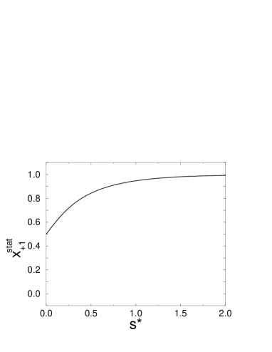
Figure 3: Stable fraction of the subpopulation, $x_{+1}^{stat}$, as a function of the strength $s^{\star}=s_{ext}/\beta T$ of the external support. (a: top) $\kappa=1$, (b: bottom) $\kappa=3$. The dashed line in (b) represents the separation line for the initial conditions, which lead either to a minority or a majority status of the subpopulation.

For $\kappa<\kappa^{c}$ (Fig. 3 a), we see that there is still only one stable solution, but with an increasing value of $s_{ext}$, the supported subpopulation exists as a majority. For $\kappa>\kappa^{c}$ (Fig. 3 b), we observe again two possible stable situations for the supported subpopulation, either a minority or a majority status. But, compared to Fig. 2(b), the symmetry between these possibilities is now broken due to the external support, which increases the region of initial conditions leading to a majority status.

Interestingly, at a critical value of $s_{ext}$, the possibility of a minority status completely vanishes. Hence, for a certain supercritical external support, the supported subpopulation will grow towards a majority, regardless of its initial population size, with no chance for the opposite opinion to be established. This situation is quite often realized in communities with one strong political or religious leader (“fundamentalistic dictatorships”), or in communities driven by external forces, such as financial or military power (“banana republics”).

The value of the critical external support, $s_{ext}^{c}$, of course depends on $\kappa$, which summarizes the internal situation in terms of the social temperature, or the population size, etc. From Eq. (3.3) we can derive the condition for which two of the three possible solutions coincide, thus determining the relation between $s_{ext}^{c}$ and $\kappa$ as follows:

$$s^{\star}_{c}=\frac{s_{ext}^{c}}{\beta T}=\frac{1}{2}\ln\left[\frac{1-\sqrt{1-\frac{\displaystyle 2}{\displaystyle\kappa}}}{1+\sqrt{1-\frac{\displaystyle 2}{\displaystyle\kappa}}}\right]+\frac{1}{2}\kappa\sqrt{1-\frac{\displaystyle 2}{\displaystyle\kappa}}$$ (27)

Fig. 4 shows how much external support is needed to paralyze a community with a given internal situation ($\kappa$) by one ruling opinion. As one can see, the critical external support is an increasing function of the parameter $\kappa$, meaning that it is more difficult to paralyse a society with strong interpersonal interactions.

Figure 4: Critical external support $s^{\star}_{c}$ (eq. 27) as a function of $\kappa$.

Let us conclude the discussion of the phase transition in the mean field limit, presented in this section. With respect to the social impact theory nowak-szam-latane-90 ; valla-nowak-94 ; lewenst-nowak-latane-92 ; kacp-holyst-96 ; kacp-holyst99 , we note that phase transitions have been not considered there, since the focus was on other phenomena so far. On the other hand, for the case of two opinions, our results well correspond to those obtained by Weidlich and Haag in a model of collective opinion formation weidl-haag-83 ; weidl-91 . There, a master equation and appropriate utility potentials are used to analyse the mean-field dynamics of interacting populations. Similar to our model, the approach used in weidl-haag-83 ; weidl-91 leads to a phase transition and a corresponding bifuraction diagram. The main difference between both models is in the interpretation of the bifurcation parameter $\kappa$. In our case, $\kappa$ results from other model parameters, e.g. from the mean “social strength” $s$ which plays a role of a coupling constant between the opinions and the communication field. In the model of Weidlich and Haag, on the other hand, this parameter is interpreted as a derivative of utility potentials. Our analytic result for the critical external support, Eq. (27), is in qualitative agreement with the stability analysis and the computer simulations presented in weidl-haag-83 ; weidl-91 .

4 Critical Conditions for Spatial Opinion Separation

In the previous section, the existence of critical parameters, such as $\kappa^{c}$ or $s_{ext}^{c}$, has been proved for a community with fast communication, where no inhomogenities in the communication field can exist. In the more realistic case, however, we have finite diffusion coefficients for the information, and the mean-field approximation, eq. (12), is no longer valid. Instead of focussing on the subpopulation sizes, we now need to consider the spatial distribution of individuals with opposite opinions.

Starting with the canonical N–particle distribution function, $P(\underline{\theta},\underline{r},t)$, eq. (10), the spatio-temporal density of individuals with opinion $\theta$ can be obtained as follows:

$$n_{\theta}(\mbox{\boldmath$r$},t) = \int\sum_{i=1}^{N}\delta_{\theta,\theta_{i}}\;\delta(\mbox{\boldmath$r$}-\mbox{\boldmath$r$}_{i})\times$$ (28)

$$\times P(\theta_{1},\mbox{\boldmath$r$}_{1}...,\theta_{N},\mbox{\boldmath$r$}_{N},t)\;d\mbox{\boldmath$r$}_{1}...d\mbox{\boldmath$r$}_{N}$$

Integrating eq. (10) according to eq. (28) and neglecting higher order correlations, we obtain the following reaction-diffusion equation for $n_{\theta}(\mbox{\boldmath$r$},t)$

$$\frac{\partial}{\partial t}\,n_{\theta}(\mbox{\boldmath$r$},t)= - \nabla\,\Big{[}n_{\theta}(\mbox{\boldmath$r$},t)\,\alpha\,\nabla h_{\theta}(\mbox{\boldmath$r$},t)\Big{]}+D_{n}\,\Delta n_{\theta}(\mbox{\boldmath$r$},t)$$

$$- \sum_{\underline{\theta^{\prime}}\neq\underline{\theta}}\Big{[}w(\theta^{\prime}|\theta)\,n_{\theta}(\mbox{\boldmath$r$},t)+w(\theta|\theta^{\prime})\,n_{\theta^{\prime}}(\mbox{\boldmath$r$},t)\Big{]}$$

with the transition rates obtained from eq. (7):

$$w(\theta^{\prime}|\theta) = \eta\,\exp\{[h_{\theta^{\prime}}(\mbox{\boldmath$r$},t)-h_{\theta}(\mbox{\boldmath$r$},t)]/T\}$$ (30)

$$w(\theta|\theta) = 0$$

With $\theta=\{+1,-1\}$, Eq. (4) is a set of two reaction-diffusion equations, coupled both via $n_{\theta}(\mbox{\boldmath$r$},t)$ and $h_{\theta}(\mbox{\boldmath$r$},t)$. Inserting the densities $n_{\theta}(\mbox{\boldmath$r$},t)$ and neglecting any external support, eq. (5) for the spatial communication field can be transformed into the linear deterministic equation:

$$\frac{\partial}{\partial t}h_{\theta}(\mbox{\boldmath$r$},t)=s\,n_{\theta}(\mbox{\boldmath$r$},t)\;-\;\beta\,h_{\theta}(\mbox{\boldmath$r$},t)\;+\;D_{h}\Delta h_{\theta}(\mbox{\boldmath$r$},t)$$ (31)

The solutions for the spatio-temporal distributions of individuals and opinions are now determined by the four coupled equations, Eq. (4) and Eq. (31). For our further discussion, we assume again that the spatio-temporal communication field relaxes faster than the related distribution of individuals into a quasi-stationary equilibrium. The field $h_{\theta}(\mbox{\boldmath$r$},t)$ should still depend on time and space coordinates, but, due to the fast relaxation, there is a fixed relation to the spatio-temporal distribution of individuals. Further, we neglect the independent diffusion of information, assuming that the spreading of opinions is due to the migration of the individuals. From Eq. (31), we find with $\dot{h}_{\theta}(\mbox{\boldmath$r$},t)=0$ and $D_{h}=0$:

$$h_{\theta}(\mbox{\boldmath$r$},t)=\frac{s}{\beta}\,n_{\theta}(\mbox{\boldmath$r$},t)$$ (32)

which can now be inserted into Eq. (4), thus reducing the set of coupled equations to two equations.

The homogeneous solution for $n_{\theta}(\mbox{\boldmath$r$},t)$ is given by the mean densities:

$$\bar{n}_{\theta}=\left\langle n_{\theta}(\mbox{\boldmath$r$},t)\right\rangle=\frac{\bar{n}}{2}$$ (33)

Under certain conditions however, the homogeneous state becomes unstable and a spatial separation of opinions occurs. In order to investigate these critical conditions, we allow small fluctuations around the homogeneous state $\bar{n}_{\theta}$:

$$n_{\theta}(\mbox{\boldmath$r$},t)=\bar{n}_{\theta}+\delta n_{\theta}\;;\quad\left|\frac{\delta n_{\theta}}{\bar{n}_{\theta}}\right|\ll 1$$ (34)

Inserting Eq. (34) into Eq. (4), a linearization gives:

$$\frac{\partial\delta n_{\theta}}{\partial t}=\left[D_{n}-\frac{\alpha s\,\bar{n}}{2\beta}\right]\;\Delta\delta n_{\theta}+\left[\frac{\eta\,s\,\bar{n}}{\beta T}-\eta\right]\;\,(\delta n_{\theta}-\delta n_{-\theta})$$ (35)

With the ansatz

$$\delta n_{\theta}\sim\exp\left(\lambda t+i\mbox{\boldmath$k$}\mbox{\boldmath$r$}\right)$$ (36)

we find from Eq. (35) the dispersion relation $\lambda(\mbox{\boldmath$k$})$ for small inhomogeneous fluctuations with wave vector $k$. This relation yields two solutions:

$$\begin{array}[]{l}\lambda_{1}(\mbox{\boldmath$k$})=-k^{2}\,C+2B\;;\;\;\lambda_{2}(\mbox{\boldmath$k$})=-k^{2}\,C\\ B=\frac{\displaystyle\eta\,s\,\bar{n}}{\displaystyle\beta T}-\eta\;;\;\;C=D_{n}-\frac{\displaystyle\alpha s\,\bar{n}}{\displaystyle 2\beta}\end{array}$$ (37)

For homogeneous fluctuations we obtain from Eq. (37)

$$\lambda_{1}=\frac{2\,\eta\,s\,\bar{n}}{\beta T}-2\,\eta\mbox{;}\quad\lambda_{2}=0\quad\mbox{for}\;\mbox{\boldmath$k$}=0$$ (38)

which means that the homogeneous system is marginally stable as long as $\lambda_{1}<0$, or $s\,\bar{n}/\beta T<1$. This result agrees with the condition $\kappa<2$ obtained from the previous mean field investigations in Sect. 3. The condition $\kappa=2$ or $B=0$, respectively, defines a critical social temperature

$$T^{c}_{1}=\frac{s\,\bar{n}}{\beta}$$ (39)

For temperatures $T<T^{c}_{1}$, the homogeneous state $n_{\theta}(\mbox{\boldmath$r$},t)=\bar{n}/2$, where individuals of both opinions are equally distributed, becomes unstable and the spatial separation process occurs. This is in direct analogy to the phase transition obtained from the Ising model of a ferromagnet. Here, the state with $\kappa<2$ or $T>T^{c}_{1}$, respectively, corresponds to the paramagnetic or disordered phase, while the state with $\kappa>2$ or $T<T^{c}_{1}$, respectively, corresponds to ferromagnetic ordered phase.

The conditions of Eq. (38) denote a homogeneous stability condition. To obtain stability against inhomogeneous fluctuations of wave vector $k$, the two conditions $\lambda_{1}(\mbox{\boldmath$k$})\leq 0$ and $\lambda_{2}(\mbox{\boldmath$k$})\leq 0$ have to be satisfied.

Taking into account the critical temperature $T^{c}_{1}$, Eq. (39), we can rewrite these conditions, Eq. (37), as follows:

$$\mbox{\boldmath$k$}^{2}\,\Big{(}D_{n}-D_{n}^{c}\Big{)}-2\,\eta\,\left(\frac{T^{c}_{1}}{T}-1\right) \geq 0$$

$$\mbox{\boldmath$k$}^{2}\,\Big{(}D_{n}-D_{n}^{c}\Big{)} \geq 0$$ (40)

Here, a critical diffusion coefficient $D_{n}^{c}$ for the individuals appears, which results from the condition $C=0$:

$$D^{c}_{n}=\frac{\alpha}{2}\;\frac{s\,\bar{n}}{\beta}$$ (41)

Hence, the condition

$$D_{n}>D^{c}_{n}$$ (42)

denotes a second stability condition. In order to explain its meaning, let us consider that the diffusion coefficient of the individuals, $D_{n}$, may be a function of the social temperature, $T$. This sounds reasonable since the social temperature is a measure of randomness in social interaction, and an increase of such a randomness lead to an increase of a random spatial migration. The simplest relation for a function $D_{n}(T)$ is the linear one, $D_{n}=\mu T$. By assuming this, we may rewrite Eq. (4) using a second critical temperature, $T_{2}^{c}$ instead of a critical diffusion coefficient $D_{n}^{c}$:

$$\mbox{\boldmath$k$}^{2}\,\mu\,\Big{(}T-T^{c}_{2}\Big{)}-2\,\eta\,\left(\frac{T^{c}_{1}}{T}-1\right) \geq 0$$

$$\mbox{\boldmath$k$}^{2}\,\mu\,\Big{(}T-T^{c}_{2}\Big{)} \geq 0$$ (43)

The second critical temperature $T^{c}_{2}$ reads as follows:

$$T^{c}_{2}=\frac{\alpha}{2\mu}\;\frac{s\,\bar{n}}{\beta}=\frac{\alpha}{2\mu}\;T^{c}_{1}$$ (44)

The occurence of two critical social temperatures $T_{1}^{c}$, $T_{2}^{c}$ allows a more detailed discussion of the stability conditions. Therefore, we have to consider two separate cases of Eq. (44): (1) $T^{c}_{1}>T^{c}_{2}$ and (2) $T^{c}_{1}<T^{c}_{2}$, which correspond either to the condition $\alpha<2\mu$, or $\alpha>2\mu$, respectively.

In the first case, $T^{c}_{1}>T^{c}_{2}$, we can discuss three ranges of the temperature $T$:

1. For $T>T^{c}_{1}$ both eigenvalues $\lambda_{1}(\mbox{\boldmath$k$})$ and $\lambda_{2}(\mbox{\boldmath$k$})$, Eq. (37), are nonpositive for all wave vectors $k$ and the homogenous solution $\bar{n}/2$ is completely stable.

2. For $T^{c}_{1}>T>T^{c}_{2}$ the eigenvalue $\lambda_{2}(\mbox{\boldmath$k$})$ is still nonpositive for all values of $k$, but the eigenvalue $\lambda_{1}(\mbox{\boldmath$k$})$ is negative only for wave vectors that are larger than some critical value $\mbox{\boldmath$k$}^{2}>\mbox{\boldmath$k$}_{c}^{2}$:

   $$\mbox{\boldmath$k$}_{c}^{2}=\frac{2\,\eta}{\mu\,T}\;\frac{T^{c}_{1}-T}{T-T^{c}_{2}}$$ (45)

   This means that, in the given range of temperatures, the homogeneous solution $\bar{n}/2$ is metastable in an infinite system, because it is stable only against fluctuations with large wave numbers, i.e. against small-scale fluctuations. Large-scale fluctuations destroy the homogeneous state and result in a spatial separation process, i.e. instead of a homogenous distribution of opinions, individuals with the same opinion form separated spatial domains which coexist. The range of the metastable region is especially determined by the value of $\alpha<2\mu$, which defines the difference between $T^{c}_{1}$ and $T^{c}_{2}$.

3. For $T<T^{c}_{2}$ both eigenvalues $\lambda_{1}(\mbox{\boldmath$k$})$ and $\lambda_{2}(\mbox{\boldmath$k$})$ are positive for all wave vectors $k$ (except $\mbox{\boldmath$k$}=0$, for which $\lambda_{2}=0$ yields), which means that the homogeneous solution $\bar{n}/2$ is completely unstable. On the other hand all systems with spatial dimension $L<2\pi/k_{c}$ are stable in this temperature region.

For case (2), $T^{c}_{1}<T^{c}_{2}$, which corresponds to $\alpha>2\mu$, already small inhomogeneous fluctuations result in an instability of the homogenous state for $T<T_{2}^{c}$, i.e we have a direct transition from the completely stable to the completely unstable regime at the critical temperature $T=T^{c}_{2}$.

That means the second critical temperature $T^{c}_{2}$ marks the transition into complete instability. The metastable region, which exists for $\alpha<2\mu$, is bound by the two critical social temperatures, $T^{c}_{1}$ and $T^{c}_{2}$. This allows us again to draw an analogy to the theory of phase transitions ulbr-schm-mah-schw-88 . It is well known from phase diagrams that the density-dependent coexistence curve $T^{c}_{1}(\bar{n})$ divides stable and metastable regions, therefore we can name the critical temperature $T^{c}_{1}$, Eq. (39), as the coexistence temperature, which marks the transition into the metastable regime. On the other hand, the metastable region is separated from the completely unstable region by a second curve $T^{c}_{2}(\bar{n})$, known as the spinodal curve, which defines the region of spinodal decomposition. Hence, we can identify the second critical temperature $T^{c}_{2}$, Eq. (44), as the instability temperature.

We note that similar investigations of the critical system behavior can be performed by discussing the dependence of the stability conditions on the “social strength” $s$ or on the total population number $N=A\bar{n}$. These investigations allow the calculation of a phase diagram for the opinion change in the model discussed, where we can derive critical population densities for the spatial opinion separation within the community.

5 Conclusions

We have discussed a simple model of collective opinion formation, based on active Brownian particles, which represent the individuals. Every individual shares one of two opposite opinions and indirectly interacts with its neighbours due to a communication field, which contains the information about the spatial distribution of the different opinions. This two-component field has a certain lifetime, which models memory effects. Furthermore, it can spread out in the community, which describes the diffusion of information. This way, every individual locally receives information about the opinion distribution, which affects its further actions: (i) the individual can keep or change its current opinion, or (ii) it can stay or migrate towards regions where its current opinion is supported. Both actions depend (a) on a social temperature, which describes the stochastic influences, and (b) on the local strength of the communication field, which expresses the deterministic influences of the decision of an individual.

For supercritical conditions within the community (e.g. supercritical population size, or supercritical external pressure, or low temperature etc.), the non-linear feedback between the individuals and the communication field, created by themselves, results in a process of spatial opinion separation. In this case, the individuals either change their opinion to match the conditions in their neighbourhood, or they keep their opinion, but migrate into regions which support this opinion.

In this paper, we have studied the critical conditions, which may lead to this separation process. In the spatially homogeneous case, which holds either for small communities or for an information exchange with infinite velocity, the communication field can be described in a mean-field approximation.

For this case, we derived a critical population size, $N^{c}$ (which is related to a critical social temperature, $T^{c}_{1}$). For $N<N^{c}$, there is a stable balance where both opinions are shared by an equal number of individuals. For $N>N^{c}$, however, one of these opinions becomes preferred, hence, majorities and minorities appear in the community. Further, we have shown how these majorities change if we consider an external support for one of the opinions. We found, that beyond some critical support, the supported subpopulation must always exist as a majority, since the possibility of its minority status simply disappears.

As a second case, we have investigated a spatially inhomogeneous communication field, which is locally coupled to the distribution of the individuals. This coupling is due to an adiabatically fast relaxation of the communication field into a quasistationary equilibrium.

Using this adiabatic approximation, we were able to derive critical conditions for a spatial separation of opinions. We found that above the critical population size (or for $T<T^{c}_{1}$), the community could be described as a metastable system, which expresses stability against small-scale pertubations. The region of metastability is bound by a second critical temperature, $T^{c}_{2}$, which describes the transition into instability, where every pertubation results in an immediate separation. Further, we obtained that the range of metastability is particularly determined by the parameter $\alpha$, which characterizes how strong an individual responses to the information received from the communication field.

Finally, we would like to note that our model of collective opinion formation only sketches some basic features of structure formation in social systems. There is no doubt, that in real human societies a more complex behavior among the individuals occurs, and that decision making and opinion formation may depend on numerous influences beyond a quantitative description. In this paper, we restricted ourselves to a simplified dynamical approach, which purposely stretches some analogies between physical and social systems. The results, however, display similarities to phenomena observed in social systems and allow an interpretation within such a context. So, our model may give rise to further investigations in the field of quantitative sociology.

References

- (1)
- (2) W. Weidlich, G. Haag (1983): Concepts and Models of Quantitative Sociology, Berlin: Springer.
- (3) S. Galam (1990): Social paradoxes of majority rule voting and renormalisation group, J. Statistical Physics 61/3-4, 943-951.
- (4) W. Weidlich (1991): Physics and Social Science – The Approach of Synergetics, Physics Reports 204, 1-163.
- (5) S. Galam (1991): Renormalisation group, political paradoxes, and hierarchies, in: W. Ebeling, M. Peschel, W. Weidlich (eds.): Models of Self-Organization in Complex Systems: MOSES, Berlin: Akademie-Verlag, pp. 53-59.
- (6) R. R. Vallacher, A. Nowak (eds.) (1994): Dynamical systems in social psychology, San Diego: Academic Press.
- (7) N. Gilbert, J. Doran (eds.) (1994): Simulating societies: The computer simulation of social processes, London: University College.
- (8) D. Helbing (1995): Quantitative Sociodynamics, Dordrecht: Kluwer Academic.
- (9) M. H. R. Stanley, L. A. N. Amaral, S. V. Buldyrev, S. Havlin, H. Leschhorn, P. Maass, M. A. Salinger, H. E. Stanley (1996): Can statistical physics contribute to the science of economics?, Fractals 4, 415-425.
- (10) J. Laherrere, D. Sornette (1998): Stretched exponential distributions in nature and economy: ”fat tails” with characteristic scales, European Physical Journal B 2, 525-539.
- (11) Challet, D.; Zhang, Y.-C. (1998): On the minority game: Analytical and numerical studies, Physica A 256, 514-532.
- (12) R. N. Mantegna, H. E. Stanley (1999): Introduction to Econophysics: Correlations & Complexity in Finance, Cambridge: Cambridge University Press.
- (13) H. Haken (1978): Synergetics. An Introduction, Berlin: Springer.
- (14) W. B. Zhang (1991): Synergetic Economics, Berlin: Springer.
- (15) D. Helbing (1993): Stochastic and Boltzmann-like models for behavioral changes, and their relation to game theory, Physica A 193, 241-258.
- (16) J.-P. Bouchaud, D. Sornette (1994): The Black-Scholes option pricing problem in mathematical finance: generalisation and extensions for a large class of stochastic processes, J. Phys. 1 France 4, 863-881.
- (17) D.S. Dendrinos, M. Sonis (1990): Chaos and Socio-spatial Dynamics, Berlin: Springer.
- (18) H.W. Lorenz (1993): Nonlinear Dynamical Equations and Chaotic Economy, Berlin: Springer.
- (19) J.A. Hołyst, T. Hagel, G. Haag, W. Weidlich (1996): How to control a chaotic economy?, J. Evolutionary Economics 6, 31-42.
- (20) J.A. Hołyst, T. Hagel, G. Haag (1997): Destructive Role of Competition and Noise for Control of Microeconomical Chaos, Chaos, Solitons & Fractals 8/9, 1489-1505.
- (21) M. Lewenstein, A. Nowak and B. Latané (1992): Statistical Mechanics of Social Impact, Phys. Rev. A 45, 703-716.
- (22) K. Kacperski, J.A. Hołyst (1996): Phase Transitions and Hysteresis in a Cellular Automata-Based Model of Opinion Formation, J. Stat. Phys. 84, 169-189.
- (23) S. Galam (1997): Rational decision making: A random field Ising model at , Physica A 238, 66–88.
- (24) A. Nowak, J. Szamrej, B. Latané (1990): From Private Attitude to Public Opinion: A Dynamic Theory of Social Impact, Psych. Rev. 97, 362-376.
- (25) F. Schweitzer, J. Bartels, L. Pohlmann (1991): Simulation of Opinion Structures in Social Systems, in: W. Ebeling, M. Peschel, W. Weidlich (eds.): Models of Selforganization in Complex Systems: MOSES, Berlin: Akademie-Verlag, pp. 236-243.
- (26) Galam, S.; Moscovici, S. (1991): Towards a theory of collective phenomena: Consensus and attitude change in groups, European Journal of Social Psychology 21, 49-74.
- (27) B. Latané, A. Nowak, J.M. Liu (1994): Dynamism, Polarization, and Clustering as Order Parameters of Social Systems, Behavioral Sci. 39, 1-24.
- (28) K. Kacperski, J.A. Hołyst (1997): Leaders and Clusters in a Social Impact Model of Opinion Formation, in: F. Schweitzer (ed.): Self-Organization of Complex Structures: From Individual to Collective Dynamics, London: Gordon and Breach, pp. 367-378.
- (29) D. Plewczynski (1998): Landau theory of social clustering, Physica A 261, 608–617.
- (30) K. Kacperski, J. Hołyst (1999): Opinion formation model with strong leader and external impact: a mean field approach, Physica A 268, 511–526.
- (31) S. Wolfram (1986): Theory and Application of Cellular Automata, Singapore: World Scientific.
- (32) L. Schimansky-Geier, M. Mieth, H. Rose, H. Malchow (1995): Structure Formation by Active Brownian Particles, Physics Letters A 207, 140.
- (33) L. Schimansky-Geier, F. Schweitzer, M. Mieth (1997): Interactive Structure Formation with Brownian Particles, in: F. Schweitzer (ed.): Self-Organization of Complex Structures: From Individual to Collective Dynamics, London: Gordon and Breach, pp. 101-118.
- (34) F. Schweitzer (1997): Active Brownian Particles: Artificial Agents in Physics, in: L. Schimansky-Geier, T. Pöschel (eds.): Stochastic Dynamics, Lecture Notes in Physics vol. 484, Berlin: Springer, pp. 358-371.
- (35) Schweitzer, F.; Ebeling, W.; Tilch, B. (1998): Complex Motion of Brownian Particles with Energy Depots, Physical Review Letters 80, 5044-5047.
- (36) W. Ebeling, F. Schweitzer, B. Tilch (1999): Active Brownian Particles with Energy Depots Modelling Animal Mobility, BioSystems 49, 17-29.
- (37) L. Lam, R. Pochy (1993): Active-Walker Models: Growth and Form in Nonequilibrium Systems, Computers in Physics 7, 534-541.
- (38) F. Schweitzer, L. Schimansky-Geier (1994): Clustering of Active Walkers in a Two-Component System, Physica A 206, 359-379.
- (39) L. Lam (1995): Active Walker Models for Complex Systems, Chaos, Solitons & Fractals 6, 267-285.
- (40) F. Schweitzer, K. Lao, F. Family (1997): Active Random Walkers Simulate Trunk Trail Formation by Ants, BioSystems 41, 153-166.
- (41) D. Helbing, F. Schweitzer, J. Keltsch, P. Molnár (1997): Active Walker Model for the Formation of Human and Animal Trail Systems, Phys. Rev. E 56, 2527-2539.
- (42) F. Schweitzer (1998): Modelling Migration and Economic Agglomeration with Active Brownian Particles, Advances in Complex Systems 1, 11-37.
- (43) F. Schweitzer, L. Schimansky-Geier, W. Ebeling, H. Ulbricht (1988): A stochastic approach to nucleation in finite systems: theory and computer simulations, Physica A 150, 261-279.
- (44) H. Ulbricht, J. Schmelzer, R. Mahnke, F. Schweitzer, F. (1988): Thermodynamics of Finite Systems and the Kinetics of First-Order Phase Transitions, Leipzig: Teubner.