Functional Dynamics II:
Syntactic structure

Abstract

Functional dynamics, introduced in a previous paper, is analyzed, focusing on the formation of a hierarchical rule to determine the dynamics of the functional value. To study the periodic (or non-fixed) solution, the functional dynamics is separated into fixed and non-fixed parts. It is shown that the fixed parts generate a 1-dimensional map by which the dynamics of the functional values of some other parts are determined. Piecewise-linear maps with multiple branches are generally created, while an arbitrary one-dimensional map can be embedded into this functional dynamics if the initial function coincides with the identity function over a finite interval. Next, the dynamics determined by the one-dimensional map can again generate a ‘meta-map’, which determines the dynamics of the generated map. This hierarchy of meta-rules can continue recursively. It is also shown that the dynamics can produce ‘meta-chaos’ with an orbital instability that is stronger than exponential. The relevance of the generated hierarchy to biological and language systems is discussed, in relation with the formation of syntax of a network.

1 Introduction

In a previous paper [1] (to be referred as I), we introduced functional dynamics to investigate the articulation process carried out on an initially inarticulate network. In the functional dynamics, objects and rules are not separated in the beginning, and we study how objects and rules appear from an inarticulate network through iterations of functions. The functional dynamics provides a simple universal model for this appearance.

In the general introduction of the paper I, we discuss five requisites for a biological system, while two of them are explicitly studied. These are the following:

• Inseparability of rule and variable ($f\circ f$).

• The articulation process from a continuous world.

In I, we investigate functional dynamics defined by

$$f_{n+1}(x)=(1-\epsilon)f_{n}(x)+\epsilon f_{n}\circ f_{n}(x)$$ (1)

The evolution of the function $f_{n}(x)$ has been studied with $n$ representing the iteration step and $\epsilon$ as a parameter. We have shown that an articulation process is generated in this 1-dimensional functional dynamics. As $f_{n}(x)$ evolves, first, type-I fixed points satisfying $f(x^{I})=x^{I}$ are formed, and then type-II fixed points satisfying $f(x^{II})=x^{I}$ are formed [1]. The articulation process is studied as a classification process of how $f_{n}(x)$ converges to distinct intervals consisting entirely of type-II fixed points. For a given value $a=f_{n}(x)$, the inverse set $I_{n}=f^{-1}_{n}(a)$ is given as an articulated class. This means that the filter articulates the continuous world $x$ into some segments according to the value $f_{n}(x)$. For such sets, $I_{n+1}\supseteq I_{n}$ holds, and the dynamics of this system is determined completely by a set of relations among these intervals as $n\rightarrow\infty$. This reduction of the degrees of freedom out of a continuous world is the articulation process. This articulation is most clearly seen in the relation between type-I and type-II fixed points. Intervals of type-II points corresponding to the same type-I fixed points are generated from an initial continuous function.

As an articulation process, a structure independent of $n$ is formed by the fixed points, while the functional values of some points change periodically in time, taking the values of different type-II fixed points successively (i.e., being mapped to the rigid structure constituted by fixed points). This periodic function provides an example of how objects and rules depend on each other, based on a rigid structure unchanged under iteration.

In the present paper, we focus on a dynamical aspect of these functional dynamics, to study how rules for dynamic change emerge through iteration of the functional mapping. With this approach, we investigate the third and forth requisites mentioned in the general introduction of I:

• Formation of a rule to change the relation among objects.

• Formation of hierarchical rules.

From our viewpoint, objects and rules emerge from the same level in which code and encoding circulate dynamically. For example, in natural language, there is a set of words and rules that forms sentences. When we assume in the beginning that the objects and rules are already separated, the theory of language has to be based on formal languages [4][5], since the structure of the language has to be studied without resorting to the objects. With the separation of words and rules, one neglects the fact that the rules have to be described by using words, while the meaning of a word has to be described by a sentence. This implies that a theory starting from a hierarchy in which words and objects are separated is not sufficient as a mathematical framework for natural language. Natural language is described as an assembly of objects, rules, meta-rules, meta-meta-rules, and so forth, while this hierarchy is not given in advance. Indeed, this process of emergence of hierarchical structure from pre-structured “something” is a common characteristic of biological systems, as is seen, for example, in the hierarchy of cell, tissue, organism, and so forth, starting from an assembly of chemical reactions. A mathematical formulation is required to study the hierarchy of the successive formation of rules at successively higher levels [6] [7].

By taking the same viewpoint as that in I, we study a network of language/objects as a functional form. With the evolution of the functional dynamics, some structure is constructed step by step. In particular, we study how a hierarchy of rules and meta-rules emerges through the iteration. Here, a structure is formed first by the configuration of fixed points, while a rule for the dynamic change of the structure is organized according to an ‘orbit’ of the functional dynamical system, and then a meta-rule is formed governing the dynamic structure generated by the orbit.

This implies that once we get a rigid (fixed-point) structure, unchanged under repeated mapping, as the elementary part of the dynamical network, hierarchical structure appears under some restrictions. Here, the rigid structure and hierarchical structure correspond to the articulated objects and the operator acting on the objects, respectively. This separation of objects and rules emerges, since we extract the rigid structure out of the functional dynamics.

The present paper is organized as follows. In Sec.2, we explain the basic properties of the functional dynamics again to facilitate its representation by the introduction of a ‘generated map’. With the generated map, it is shown in Sec.3.1, that a 1-dimensional map is embedded in the functional dynamics. This map works as a rule governing the change of the functional values over some intervals. In Secs.3.1 and 3.2, piecewise linear maps called the Nagumo-Sato map and the ‘multi-branch Nagumo-Sato map’ are naturally embedded in the functional dynamics. In Sec.3.3 a larger class of 1-dimensional maps is embedded into our functional map. This implies that chaotic functional dynamics is possible in our system. By choosing a suitable initial condition, it is shown in Sec.4 that the functional dynamics can form a hierarchical structure. A meta-rule for the change of the functional values is formed which changes according to the (chaotic) dynamics generated by the 1-dimensional map. The maps can be nested recursively and generate higher level meta-maps successively. In Sec.5, we discuss syntactic structure derived from this functional dynamics, and the relevance of our results to the 3rd and 4th requisites of biological systems, mentioned above.

2 Model

The functional map Eq. (1) has the form

$$f_{n+1}(x)=F(f_{n}(x),f_{n}\circ f_{n}(x)).$$ (2)

Here we study some characteristics of this functional equation with a 1-dimensional $f_{n}(x)$. In connection with our motivation for biological systems and language structure, the function $f_{n}(x)$ is considered to represent an abstract relation network, while $f_{n}\circ f_{n}(x)$ provides a self-referential term. Since we are interested in modeling the situation in which code and encoding are not separated, $f_{n}(x)$ represents a projection from a set into itself.

First, we discuss two characteristic properties of this equation:

• If $x^{\prime}$ and $x^{\prime\prime}$ have the same value $f_{n}(x^{\prime})=f_{n}(x^{\prime\prime})$ at $n$, the subsequent evolutions of $f_{m}(x^{\prime})$ and $f_{m}(x^{\prime\prime})$ (with $m>n$) are identical, because dynamics are determined completely by the function $f_{n}(x)$.

• The equation (1) can be split as

  $$\left\{\begin{array}[]{lcl}f_{n+1}(x)&=&g_{n}(f_{n}(x))\\ g_{n}(x)&=&F(x,f_{n}(x)).\end{array}\right.$$ (3)

The first property above implies the ability of articulation of this system. Once $f_{n}(x)$ identifies $x^{\prime}$ and $x^{\prime\prime}$ as the same thing, the two points evolve in the same way. The second property provides a novel viewpoint to study this model. With this separation, one can say that a point $f_{n}(x^{\prime})$ evolves under $g_{n}(x)$, which is generated from $f_{n}(x)$ itself. This is a characteristic property of this functional equation. Given $f_{n}(x)$, a map $g_{n}(x)$ is determined. The $f_{n}(x)$ evolves to $f_{n+1}(x)$ under the map and $g_{n+1}(x)$ is determined. In this paper, the term ‘function’ is used to represent $f_{n}(x)$, while a ‘generated map’ is used in reference to $g_{n}(x)$.

If $f(x^{\prime})$ is a fixed point at $x^{\prime}$ (which does not mean a fixed function as a whole), the generated map of $f(x^{\prime})$ is a fixed generated map at the point $x^{\prime}$. To study the functional dynamics, we first study a fixed generated map $g(x)$ and see how other points $x^{\prime\prime}$ evolve under this generated map (Sec.3). Second, we study the case in which $g_{n}(x)$ itself changes in time, by taking a suitable initial configuration of $f_{0}(x)$. There, a hierarchical structure (meta-map) is considered (Sec.4).

For simplicity, we impose one more restriction on (2), following I. We assume that, if the relation $f(x^{\prime})$ is fixed, it satisfies the relation $f(x^{\prime})=f\circ f(x^{\prime})$. This condition implies that the change of $f(x^{\prime})$ vanishes when the self-reference of a function agrees with the function itself. The simplest model of this type is (1), obtained by choosing the form

$$F(x,y)=(1-\epsilon)x+\epsilon y,$$ (4)

with $0<\epsilon<1$. (The case with a general form for $F(x,y$) is briefly discussed in Appendix A and will be discussed in a future paper.)

For the type of model we study, the dynamics relax toward the self-consistent relation $f(x^{\prime})=f\circ f(x^{\prime})$. For the remainder part of this paper, we focus on the functional dynamics (1). In this case, the generated map is given by $g_{n}(x)=(1-\epsilon)x+\epsilon f_{n}(x)$.

Now we obtain two useful properties:

• A value $f_{n}(x^{\prime})$ which satisfies the condition $f_{n}(x^{\prime})=f_{n}\circ f_{n}(x^{\prime})$ is a fixed point.

• There is a transformation $T$ which satisfies the condition $F\circ T=T\circ F$. (The explicit form of $T$ is discussed below.)

Here, all the points $x^{I}$ which satisfy $f(x^{I})=x^{I}$ are fixed points of the functional equation(1). Since all points $x$ with an identical value $f(x)$ evolve identically, all the points $x^{II}$ that satisfy $f(x^{II})=x^{I}$ are again fixed points. For convenience, we have classified (see I) these fixed points as

• $x^{I}$ is a type-I fixed point with $f_{n}(x^{I})=x^{I}$ .

• $x^{II}$ is a type-II fixed point with $f_{n}(x^{II})=x^{I}\neq x^{II}$.

A type-I fixed point is a point at which $f_{n}(x)$ intersects the identity function. This ‘type’ is extended to arbitrary type-$N$. We define a type-$N$ point as a point which satisfies the condition $f(x^{N})=x^{N-1}$, after the transient in the functional dynamics has died away. Here $x^{N}$ represents a type-$N$ point. Although type-I and II points are fixed points, type-$N$ ($N>2$) points cannot be fixed points. In fact, if $x$ is a fixed point and $y=f(x)$, the fixed point condition is written $y=f(y)$, which means $y$ is a type-I fixed point and $x$ is a type-I or II fixed point.

In I, we introduced the concept of a ‘self-contained section’ (SCS), which is defined as a connected interval $I$ such that $f(I)\subset I$, while no connected interval $J\subset I$ satisfies $f(J)\subset J$, and $f(I+\delta)\subset I+\delta$ for arbitrary small $\delta$, either. Here, we extend this definition to introduce the ‘closed section’ (CS) and ‘closed generated map’ (CGM). A CS is defined as a set $I$ such that $f(I)\subset I$ (where $I$ is not necessarily connected), while a CGM is defined as a set $J$ such that $g(J)\subset J$ (where $J$ is not necessarily connected). In Eq.(1), if $f_{0}(I)\subset I$, then $f_{n}(x)\in I$ for all $n$, and $I$ is a CS.

Now let us return to the transformation $T$. The dynamics of this functional equation is invariant by the transformation $T$:

$$\left\{\begin{array}[]{lcl}ax+b&\rightarrow&X\\ af_{n}(x)+b&\rightarrow&F_{n}(X).\end{array}\right.$$ (5)

In fact, Eq.(1) assumes the form of an operation of taking a weighted average of $f_{n}(x^{\prime})$ and $f_{n}\circ f_{n}(x^{\prime})$. Thus, the functional dynamics are invariant under a scaling transformation in which $x$ and $y=f(x)$ are multiplied by the same factor and shifted by the same value. This invariance means that $T$ and $F$ commute ($T\circ F=F\circ T$). Under this transformation, a connected CS (CGM) $(x_{1},x_{2})$ is shifted to $(ax_{1}+b,ax_{2}+b)$ giving a new CS (CGM). The above invariance will be used to embed a 1-dimensional map into this functional dynamics in Sec.3 and to construct a meta-map in Sec.4.

3 1-Dimensional Map in Functional Dynamics

3.1 General Properties

In I, we found that the function $f_{n}(x)$ does not converge to a fixed function as $n\rightarrow\infty$ for some initial functions. For example, for the initial function $f_{0}(x)=rx(1-x)$, $f_{n}(x)$ does not converge to a fixed function for some range of parameter $r$ referred to as the R (random) phase in I, where the number of discontinuous points of $f_{n}(x)$ and the length of $f_{n}(x)$ increases in proportion to $M$, the number of mesh points adopted for the numerical calculation.

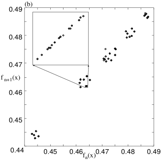
Figure 1: (a) The $f_{50000}(x)$ $(0.4<x<0.5)$ for random initial $f_{0}(x)$ with $M=6000$ and $\epsilon=0.02$. It consists of type-I fixed points, type-II fixed intervals and some periodic points. (b) A part of the return map of (a) for all $(f_{n}(x),f_{n+1}(x))$ $(n=50000-50050)$. The return map consists of some points and lines that have slope $(1-\epsilon)$ (in the inset).

Recalling that the $f_{n}(x)$ for large $n$ looks almost random in the R phase, we have also computed $f_{n}(x)$ from Eq.(1) using random initial conditions, as an extreme case. For such initial conditions, we divide the interval $[0,1]$ into $M$ intervals as ($[i/(M-1),(i+1)/(M-1)]$) and choose the value of $f_{n}(i)\in[0,1]$ randomly. An example of $f_{\infty}(x)$ for an interval $x$ and the return map $(f_{n}(x),f_{n+1}(x))$ for the interval are displayed in Fig.1. Here, $f_{n}(x)$ mainly consists of many flat intervals with the same value, while for some points $x$, $f_{n}(x)$ changes periodically in time. As plotted by the return map, it is found that the periodic dynamics obey a certain rule. As shown in the inset of Fig.1(b), a clear piecewise-linear structure is visible in the return map. In this section, we study how this type of return maps is generated (Sec.3.2) and investigate the class of maps that can appear with these functional dynamics (Sec.3.3).

A fixed generated map can be constructed from type-I and type-II fixed points. This fixed generated map can act as a 1-dimensional map $g(x)$. To extract the temporal change of other $x$ points, it is useful to think of the interval $I$ as the union of three parts: $I=I_{map}\sqcup I_{driven}\sqcup I_{rest}$. Here $f(x)$ with $x\in I_{map}$ generates a fixed generated map $g(x)$ for $f_{n}(x)$ with $x\in I_{driven}$ and $f_{n+1}(x)=g(f_{n}(x))$ with $x\in I_{driven}$. Since $f(I_{map})$ is a fixed function, $f(I_{driven})\subset I_{map}$ and $f(I_{rest})\subset I_{driven}\sqcup I_{rest}$.

First, we assume there exists only one type-I fixed point $x^{I}$ ($f(x^{I})=x^{I}$) and one type-II fixed point $x^{II}$ and that $f(x^{II})=x^{I}$. The generated map at $x=x^{II}$ is $g(x^{II})=(1-\epsilon)x^{II}+\epsilon x^{I}$, which can be rewritten as $g(x)=(1-\epsilon)(x-x^{I})+x^{I}$ by inserting $x=x^{II}$.

Next, we assume that there is an interval $I_{map}$ consisting entirely of a single type-I fixed point and corresponding type-II fixed points, which satisfy $f(x^{\prime\prime})=x^{I}$ for $x^{\prime\prime}\in I_{map}$. Assuming the existence of such an interval, the generated map is given by $g(x)=(1-\epsilon)(x-x^{I})+x^{I}$ for this interval $(x\in I_{map})$. The map $g(x)$ is a line with a slope $1-\epsilon$ that intersects the type-I fixed point. This line that is used as generated map is determined by the configuration of type-II fixed points. If the interval $I_{map}$ is continuous, for $x\in I_{driven}$ all $f_{n}(x)$ evolve to $f_{\infty}(x)=x^{I}$.

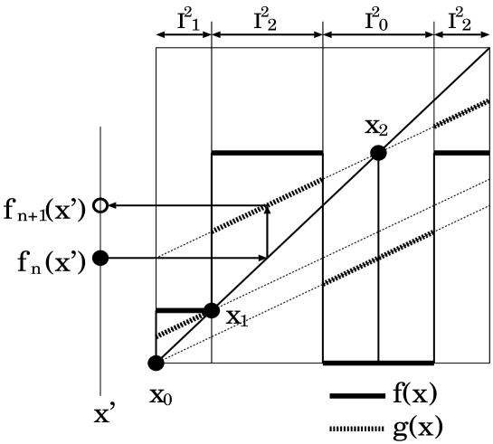
Figure 2: An example of three type-I fixed points ($x_{0}<x_{1}<x_{2}$) and $f(x)$ for $x\in I$. The map $g(x)$ is represented by the dotted line. $g(x)^{\prime}=(1-\epsilon)$ and is constant. the dynamics of another point $f_{n}(x^{\prime})\in I$ is determined by $g(x)$.

Now consider the more general case in which an interval $I_{map}$ consisting of several type-I fixed points and several subintervals of type-II points that are mapped to one of the type-I fixed points. In this case, the generated map is determined by the arrangement of type-I and type-II fixed points. This map is a piecewise linear function with slope $1-\epsilon$, which intersect the type-I fixed points (see Fig.2). Here, we consider the following two cases for the configuration of type-I fixed points:

• There exist countable number of type-I fixed points (Sec.3.2).

• There exist countable number of type-I fixed intervals (Sec.3.3).

A type-I fixed interval is a connected interval $[a,b]$ on which $f(x)=x$ for all $x\in[a,b]$. A type-I fixed point is the limiting case of a type-I fixed interval (i.e., that in which $a=b$).

Let us denote the ordered set of type-I fixed points by $I^{1}\equiv\{x_{0},x_{1},\ldots,x_{n-1}\}$ where $i<j$ implies $x_{i}<x_{j}$. The ordered set of type-I fixed intervals are denoted in the same way as the fixed points, as $I^{1}\equiv\{I^{1}_{0},I^{1}_{1},\ldots,I^{1}_{n-1}\}$, where $i<j$ implies $\max I^{1}_{i}<\min I^{1}_{j}$.

Depending on the configuration of type-I and type-II fixed points, a one-dimensional map is generated, which acts as a fixed CGM for a point $f_{n}(x^{\prime})$ for $x^{\prime}\in I_{driven}$ In the next subsection, we study the case with isolated type-I fixed points, while in Sec.3.3 we discuss the case with type-I fixed intervals.

3.2 Case with Countable Type-I Fixed Points

In this subsection, we consider the case with a finite or countably infinite number of type-I fixed points. As shown in I, the function $f_{n}(x)$ often tends to approach a piecewise constant function, consisting of a discrete set of type-I fixed points and several intervals of type-II fixed points at which $f(x)$ assumes the same value. Thus the existence of such type-I fixed points and type-II intervals is common in our model ([1] and Fig.1(a)).

Corresponding to type-I fixed points $x_{i}$, we define sets of type-II fixed points $I^{2}_{i}$ to be those satisfying $f(I^{2}_{i})=x_{i}$, where $I^{2}_{i}$ is not necessarily connected and consists of several intervals in general. Since $f(x)$ is a single-valued function, there is no intersection among $I^{2}_{i}$ and $I^{1}$. The union of type-II fixed intervals ($\cup_{i}I^{2}_{i}$) is denoted as $I^{2}$. Now, the interval $I$ is the union of $I^{1},I^{2},I_{driven}$ and $I_{rest}$ ($I=I^{1}\sqcup I^{2}_{0}\sqcup I^{2}_{1}\sqcup\cdots\sqcup I^{2}_{n-1}\sqcup I_{driven}\sqcup I_{rest}$). Following the argument in the last subsection, the generated map in the interval $I_{map}$ has the form

$$g(x)=\left\{\begin{array}[]{cccclcl}g[0](x)&=&(1-\epsilon)(x-x_{0})+x_{0}&\mbox{for }&x\in I^{2}_{0},&\mbox{where }&f(I^{2}_{0})=x_{0}\\ g[1](x)&=&(1-\epsilon)(x-x_{1})+x_{1}&\mbox{for }&x\in I^{2}_{1},&\mbox{where }&f(I^{2}_{1})=x_{1}\\ \vdots&&\vdots&&\vdots&&\vdots\\ g[n-1](x)&=&(1-\epsilon)(x-x_{n})+x_{n-1}&\mbox{for }&x\in I^{2}_{n-1},&\mbox{where }&f(I^{2}_{n-1})=x_{n-1}\end{array}\right.$$ (6)

where $[i]$ denotes a line corresponding to the type-I fixed point $x_{i}$. Each $g[i]$ is referred to as an ‘$i$-branch’.

As discussed above, this generated map acts as the evolution rule for points $x^{\prime}$ that are mapped to one of the type-II fixed points [i.e., $f_{n}(x^{\prime})\in I^{2}_{i}$, or, in other words, $f_{n+1}(x^{\prime})=g(f_{n}(x^{\prime}))=(1-\epsilon)f_{n}(x^{\prime})+\epsilon x^{I}$ (see Fig.2)].

The combination of some type-I fixed points and an set of type-II fixed intervals satisfying certain conditions can give a CGM. Here we assume there exist $n$ type-I fixed points ($x_{0}<x_{1}<\cdots<x_{n-1}$), and the points in the interval $(x_{0},x_{n-1})$ are assumed to be mapped to one of the type-I fixed points. Then, according to (6), for $i=0,1,\ldots,n-1$, $g[i](x^{\prime})\in(x_{0},x_{n-1})$ for all $x^{\prime}\in I^{2}_{i}$. As a total, $g(I^{2})\subset I^{2}$, and the set on which $g(x)$ is defined is a CGM. Thus, for $x\in I_{driven}$, the evolution of $f_{n}(x^{\prime})$ $\in I^{2}_{i}$ is determined by the CGM. This $f_{n}(x^{\prime})$ is included in a type-II fixed interval, and thus $f_{n}(x^{\prime})$ can be called type-III. The domain of $f_{n}(x^{\prime})\in I^{2}_{i}$ is denoted as $I^{3}$ ($=I_{driven}$). Now, the interval $I$ can be written as $I^{1}\sqcup I^{2}\sqcup I^{3}\sqcup I_{rest}$. Here we call this type of configuration that generates a closed 1-dimensional map as ‘unit-I’. The situation is drawn schematically in Fig.3.

For example, we assume that there are two type-I fixed points, $x_{0}$ and $x_{1}$ ($I^{1}=\{x_{0},x_{1}\}$). We divide the interval $I=[x_{0},x_{1}]$ into $I^{1},I^{2}_{0},I^{2}_{1},I^{3}$ and $I_{rest}$. Since $f(x)$ has only two values, $x_{0}$ and $x_{1}$, on $I^{2}$, $g(x)$ has a ‘0-branch’ and a ‘1-branch’. The map $g(x)$ has the same slope, ($1-\epsilon$), at each point $x\in I^{2}$. This class of map includes the Nagumo-Sato map [8].

The Nagumo-Sato map is given by the equation

$$x_{n+1}=kx_{n}+w(\bmod 1),$$ (7)

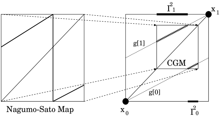
Figure 4: An embedding of the Nagumo-Sato Map. A transformation multiplying $\epsilon$ and moving $(1-w)$ along the $x$ and $y=f_{n}(x)$ directions embeds a map into $g(x)$ for $\epsilon=1-k$.

with $0<k<1$ and $0<w<1$. This map has two branches with the same slope $k$ for the interval $[0,(1-w)/k]$ (the first branch) and $[(1-w)/k,1]$ (the second branch) (see Fig.4). To have these two branches, we need two intervals of type-II fixed points. With the aid of transformation (5), the domain of $f_{n}(x)$ is restricted to [0, 1], where two type-I fixed points are situated at 0 and 1, without loss of generality. Our purpose here is to show that certain intervals $I^{2}_{0}$ and $I^{2}_{1}$ can generate a map of the form (7).

With the transformation (5), the slope $k=(1-\epsilon)$ is conserved. Transforming (7) by multiplying by $\epsilon$ and shifting by $1-w$ along $x$ and $y=f_{n}(x)$-directions, we can embed the Nagumo-Sato map (of the interval size $\epsilon$) into $g(x)$. The required condition is $I^{2}_{0}=[(1-w)/(1-\epsilon),1-\epsilon+w]$ and $I^{2}_{1}=[1-w,(1-w)/(1-\epsilon)]$ (See Fig.4). This map $g(x)\in[1-w,1-w+\epsilon]$ becomes a CGM. Note that this situation can generally arise without choosing a very special initial function. This is why the functional dynamics from arbitrary initial conditions often lead to a periodic cycle governed by the Nagumo-Sato map, as in Fig.1.

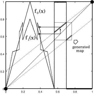
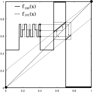
Figure 5: Time evolution of $f_{n}(x)$. The function $f_{n}(x)$ is divided into two parts, the map area and the rest. Here, fixed intervals produce the Nagumo-Sato map, and the dynamics of $f_{n}(x)$ which is mapped to the square is determined by the map. Here $a=0.7$,$\epsilon=0.2$. At the square, the generated map $g(x)$ has the same properties as the map $x_{n+1}=0.8x_{n}+0.44$. (a) $f_{0}(x)$ and $f_{1}(x)$ are plotted. $f_{0}(x)$ is chosen as described in the text. The dynamics of the function mapped to the square region is determined by the generated map, while the remaining part converges to a type-II fixed point. (b) $f_{100}(x)$ and $f_{101}(x)$ are plotted. All points converge to fixed or periodic points. The periodic points are determined by the Nagumo-Sato map. Each point is period-3, and as a whole $f_{n}(x)$ is a period-3 function.

An example of our simulations is displayed for $\epsilon=0.2$ and $w=0.44$ in Fig.5, where the discontinuous point ($a=(1-w)/(1-\epsilon)$) of the Nagumo-Sato map is located at 0.7. In the simulation, the initial configuration of $f_{n}(x)$ was given by

$$f_{0}(x)=\left\{\begin{array}[]{cl}0&x\in[a,1)\\ 1-\frac{2}{(1-\epsilon)a}|x-\frac{(1-\epsilon)a}{2}|&x\in[0.0,(1-\epsilon)a)\\ 1&x\in[(1-\epsilon)a,a),1\end{array}\right.$$ (8)

With the evolution of our functional dynamics, the function $f(x)$ for $x\in I^{2}_{0},I^{2}_{1}$ generates the Nagumo-Sato map. The remaining part ($I_{rest}$) of the interval (i.e., that which is mapped according to a distorted tent map) folds by itself (see I) and if it is mapped to a value in $I^{2}_{0}$ or $I^{2}_{1}$, it subsequently evolves under the generated Nagumo-Sato map. Figure 5(b) shows snapshots of the function $f_{n}(x)$ for $n=100,101$. The function converges to a periodic function as a whole. The period of the cycle is derived from the generated map. The functional values of two different points $x^{\prime}$ and $x^{\prime\prime}$ having the common periodic cycle changes synchronously ($f_{n}(x^{\prime})=f_{n}(x^{\prime\prime})$), because the difference in $f_{n}(x)$ values decreases during the transient process before $f_{n}(x^{\prime})$ and $f_{n}(x^{\prime\prime})$ are attracted to the periodic motion, and also the Nagumo-Sato map has a contraction property (with slope less than 1), in each branch. As $n\rightarrow\infty$, the points in the interval $I$ are contained in either $I^{1},I^{2}$ or $I^{3}$, and $I_{rest}$ vanishes.

In general, an $f(x)$ with (at least) two type-I fixed points has a potential to possess a Nagumo-Sato map as a generated map. To consider a general situation with multiple type-I points and/or with several type-II intervals, we define the ‘multi-branch Nagumo-Sato map’ by (6). In this case, $g(x)$ has the same slope $(1-\epsilon)<1$ for all $x$. This type of map can be generated generally from random initial conditions. In fact, in the inset in Fig.1(b), $g(x)$ consists of several branches with the same slope $1-\epsilon$.

With the multi-branch Nagumo-Sato map, a function $f_{n}(x)$ periodic in $n$ with an arbitrary period can exist for all $\epsilon$. If $g(x)$ with a period-$m$ attractor is given, we denote a value of a type-III $f_{n}(x^{\prime})$ as $a_{n+1}=g(a_{n}),n\bmod m$. Then a new attractor with period-$m+1$ is obtained by choosing an initial function to have two new branches properly. We can arrange branches $[i]$ and $[j]$ to satisfy the conditions that $g_{n}[i](a_{m-1})=a_{m}$ and $g_{n}[j](a_{m})=a_{0}$ for an arbitrary periodic orbit.

By choosing initial functions suitably, we can have rather complex dynamics based on the multi-branch Nagumo-Sato map. In Appendix B, the coexistence of multiple attractors is demonstrated, while it is also shown that $g(x)$ can have countably infinite attractors by suitably choosing the initial conditions to generate the multi-branch Nagumo-Sato map.

In the argument above, the function $g(x)$ is defined at a countable number of points of $x$ (i.e., the attractor of the generated map $x_{n+1}=g(x_{n})$ has a measure zero basin). However, if all type-II fixed points are in a continuous type-II fixed interval, each attractor has a finite measure basin. When $f_{0}(x)$ is a random function, such continuous intervals are formed. In fact, a multi-branch Nagumo-Sato map is often generated from random or other initial functions. In general, the width of each branch is not identical, and a complicated combination of branches is generated. As shown in I, intervals of type-II fixed points form a fractal structure. Hence, branches in the generated map have an infinite number of segments with a fractal configuration, in general. Thus $f_{n}(x)$ can evolve with a complicated cycle that may be of infinite period.

3.3 Case with Continuous Type-I Fixed Intervals

In the cases considered to this point, the generated map in the functional dynamics (1) cannot exhibit chaotic instability, in the sense that the slope of the map is less than 1 for almost all points. Except for a (countable) set of discontinuous points, all generated maps have a slope $1-\epsilon$. Here we study how a generated map can have a larger class of 1-dimensional maps that allow for chaotic instability.

To study this class of functional dynamics, we extend our consideration to the case with a continuous set of type-I fixed points, i.e., with an interval of type-I fixed points ($f(x^{\prime})=x^{\prime}$ for all $x^{\prime}\in I^{1}_{i}$). The existence of such an interval is exceptional in this functional map system, in the sense that it is almost impossible to produce such an interval by the evolution (1) unless the initial function does not include such an interval. Indeed, a monotonically increasing function converges to a step function, and a single-humped function tends to converge to a function consisting of isolated type-I fixed points and continuous intervals of type-II fixed points[1].

Although an initial function evolving into a function possessing type-I fixed intervals is rather rare in functional space, such an initial function may have some meaning in our model. The region in which $f(x)=x$ is nothing but a region where the input is accepted ‘as it is’. With regard to language, it is not absurd to assume that some external input is transferred without being modified or articulated. We can consider that the initial intervals satisfying $f_{0}(x)=x$ represent regions corresponding to such external input. Other regions of $f(x)$ that are mapped to this part process this external input according to the functional dynamics. In addition to this meaning, the situation in which there exists a continuous set of type-I fixed points is convenient for studying the hierarchy of meta maps, to be discussed in the next section. Accordingly, we assume the existence of type-I fixed intervals.

Then, we define sets of type-II fixed points in the same way as in the last subsection. The type-I fixed intervals are labeled as $I^{1}_{0},I^{1}_{2},\ldots,I^{1}_{n-1}$. Now, $I^{2}_{i}$ is defined as an interval where $f(x^{\prime})\in I^{1}_{i}$ for all $x^{\prime}\in I^{2}_{i}$ (See Fig.6). Although in the last subsection, we considered the case in which $f(x)$ is a constant function over an interval $I^{2}_{i}$, in the present case, each $f(I^{2}_{i})$ can have various values in the range of $I^{1}_{i}$. Let us write $f(I^{2}_{i})$ as $f[i](x)$. The generated map from the interval $I_{map}$ with fixed function has the form

$$g(x)=\begin{array}[]{cccc}\cup_{i}g[i](x)=&\cup_{i}(1-\epsilon)(x-f[i](x))+f[i](x)&x\in I^{2}_{i},&f[i](I^{2}_{i})\subset I^{1}_{i}\\ \end{array}$$ (9)

This function $g[i](x)$ is bounded both from above and below, because $f[i](x)$ has a possible minimum value $\min I^{1}_{i}=a$ and possible maximum value $\max I^{1}_{i}=b$, $(1-\epsilon)(x-a)+a\leq g[i](x)\leq(1-\epsilon)(x-b)+b$ (see Fig.6). It is natural to call this function $g[i](x)$ within this bounded area the ‘$i$-branch’, in analogy to the last subsection. For each type-I fixed point $x_{i}$, the generated map is given by $(1-\epsilon)(x-x_{i})+x_{i}$, although $x_{i}$ here can change continuously.

Consider the union of $n$ type-I fixed intervals $I^{1}=I^{1}_{0}\sqcup I^{1}_{2}\sqcup\cdots\sqcup I^{1}_{n-1}$. If type-II fixed intervals are within an interval $(\min I^{1},\max I^{1})$ and the condition $g(I^{1}\sqcup I^{2})\subset I^{1}\sqcup I^{2}$ is satisfied, the interval $I^{1}\sqcup I^{2}$ is a CGM (unit-I). Here, in a type-II fixed point interval corresponding to a type-I fixed point interval, the generated map $g(x)=(1-\epsilon)x+\epsilon f(x)$ no longer has a constant slope. Rather the slope $g^{\prime}(x)=(1-\epsilon)+\epsilon f^{\prime}(x)$ varies with $x$.

Following the argument in the last section, we start from the case with two type-I intervals. Now, we divide the interval $I$ into a type-I fixed interval $I^{1}$ and a type-II fixed interval $I^{2}$ ($I_{map}=I^{1}\sqcup I^{2}$). Then, the interval $I^{1}$ is divided into two parts, $I^{1}_{0}$ and $I^{1}_{1}$. Without loss of generality, we can take $\min I^{1}_{0}=0$ and $\max I^{1}_{1}=1$. The fixed function consisting of type-II fixed points is determined as $f[0](x)\in I^{1}_{0}$ for $x\in I^{2}_{0}$ or $f[1](x)\in I^{1}_{1}$ for $x\in I^{2}_{1}$. Then the generated map $g(x)$ is given by

$$g(x)=\left\{\begin{array}[]{cl}x&x\in I^{1}\\ g[0](x)=(1-\epsilon)x+\epsilon f[0](x)&x\in I^{2}_{0}\\ g[1](x)=(1-\epsilon)x+\epsilon f[1](x)&x\in I^{2}_{1}\end{array}\right.$$ (10)

The area where the generated map can exist is denoted by the dotted area in Fig.6. Any 1-dimensional map included within the dotted area can be embedded into our functional map by choosing the configuration of the type-II fixed function within the shadowed area. Since any function can be embedded in the dotted area, it is possible to have a case with $|g^{\prime}(x)|>1$.

In Fig.6, there are regions where $g(x)\in I^{1}$. If the generated map exists in such a region, a point evolving as a type-III point may be absorbed into this region and become a type-II point. Indeed, when the point is mapped into this region, $f_{n+1}(x^{\prime})\in I^{1}$ is satisfied, and the point $x^{\prime}$ becomes a type-II fixed point. On the other hand, if $g(x)\in I^{2}$, a type-III point remains a type-III during the entire evolution, and it never becomes a type-II fixed point.

Is there some restriction on the possible form of a generated map allowed by the present functional dynamics? As discussed in Appendix C, there is some restriction according to the present embedding of the generated map. However, as is also discussed in that Appendix, an arbitrary 1-dimensional map can be embedded as a generated map by considering a two-step iteration, i.e., as a map to generate $f_{n+2}(x)$ from $f_{n}(x)$.

4 Meta-Map in Functional Dynamics

In Sec.3, we have shown how a 1-dimensional generated map is formed by a suitable configuration of type-I and type-II fixed points. In the example, the 1-dimensional map is explicitly constructed with the condition $g(I^{1}\sqcup I^{2})\subset I^{1}\sqcup I^{2}$. We call the interval $U^{1}\sqcup U^{2}$ a ‘unit-I’ $U^{1}$. In this case the generated map $g_{n}(x)$ is fixed in time. However, the CGM condition ($g(J)\subset J$) does not necessarily impose the condition for the ‘unit-I’. Then, $g_{n}(x)$ is not necessarily a fixed function. In this section we consider such case in which a generated map changes dynamically in time.

In the situation discussed in Sec.3, in order for there to exist a generated map to determine the dynamics of the type-III points, it is essential that the map stays within a bounded area. The type-I fixed intervals are areas where type-II fixed points can exist, from which the type-II fixed function never leaves. The configuration of type-I and II fixed points determines bounded areas in which the generated map remains as a branch. The type-II fixed function determines a generated map within the bounded areas (See Fig.6).

In the last section, we considered the situation in which the dynamics of the type-III point determined by $g(x)$ evolves within the interval $U^{1}$, according to the type-II and corresponding type-I fixed points. This process can be extended hierarchically. In this section, we consider a unit-I instead of a type-I fixed interval and a type-III point instead of a type-II point, to see the dynamics of $f_{n}(x)$ for $x$ determined by the type-III point.

The unit-I ($\in U^{1}$) determines an interval where type-II and III points can exist. The unit $U^{1}$ is $I^{1}\sqcup I^{2}$. Thus, $\{f_{n}(x)|f_{n}(x)\in U^{1},x\in I^{2}\sqcup I^{3}\}$ consists entirely of type-II fixed points and type-III points. Here, the dynamics of the type-III points are determined by a CGM, and their motion is confined within this region. Thus, we replace the type-I fixed interval with unit-I by the transformation (5). In case considered in the last section, the configuration of type-I fixed intervals determines where the branches exist. Here, the arrangement of unit-I determines where the branches of the generated map exist.

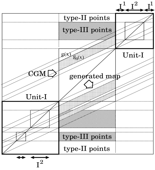
Figure 7: The hierarchical arrangement of a ‘meta-map’. The shaded area is a region where type-III points can exist and the dotted branch indicates a region where the generated map, derived from type-III points, can exist. A generated map in $I^{3}$ has an $n$ dependence ($g_{n}(x)$).

First, we elucidate the branch structure determined by a unit-I (See.Fig.7). These branches are derived from type-I and II points. As noted, at the branch derived from a type-I point, a 1-dimensional map is given according to the configuration of the type-II fixed function. In the same way, at a branch derived from type-II points, a bounded map $g_{n}(x)$ exists according to the configuration of the type-III function. Since $\{f_{n}(x)|x\in I^{3}\}$, consisting of the type-III points, depends on $n$, the generated map, $g_{n}(x)=(1-\epsilon)x+\epsilon f_{n}(x)$, also depends on $n$:

$$\begin{array}[]{l}\left\{\begin{array}[]{cll}f(x)&&x\in I^{2},f(x)\in I^{1}\\ g(x)&=(1-\epsilon)x+\epsilon f(x)&x\in I^{2}\\ \end{array}\right.\\ \left\{\begin{array}[]{cll}f_{n}(x)&=g(f_{n-1}(x))&x\in I^{3},f_{n}(x)\in I^{2}\\ g_{n}(x)&=(1-\epsilon)x+\epsilon f_{n}(x)&x\in I^{3}\end{array}\right.\end{array}$$ (11)

Here, $g_{n}(x)$ is generated from the type-III function and change with time step $n$. The point $f_{n}(x^{\prime})\in I^{3}$ evolves according to $g_{n}(x)$ ($f_{n+1}(x^{\prime})=g_{n}(f_{n}(x^{\prime}))$). Since $g_{n}(x)$ is not a fixed function, it represents a change of rules. Accordingly, we call this type of map a ‘meta-map’. By using these branches, we can construct a new CGM consisting of $g(x)$ and $g_{n}(x)$. The type of point $x$, which evolves under the CGM, can change in time. The interval $I$ can be written $I^{1}\sqcup I^{2}\sqcup I^{3}_{n}\sqcup I^{4}_{n}\sqcup I_{rest}$. Now, $I^{3}$ and $I^{4}$ have the suffix $n$.

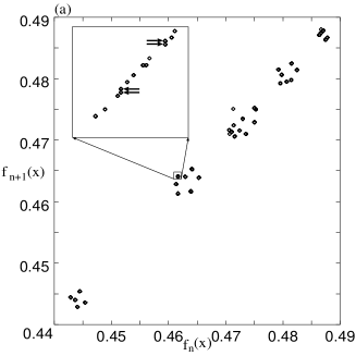
Figure 8: (a) Another close up of the return map of Fig.1(a). At the points $x^{\prime}$ indicated by arrows, $g_{n}(x^{\prime})$ has two values. (b) Time evolution of $f_{n}(x^{\prime})$ for $10000<n<10300$, which is determined by the meta-map and has a period 111. The function $f_{n}(x^{\prime})$ is a type-IV point at the steps $n$ plotted with squares $\Box$, while it is type-III otherwise.

When the dynamics of type-III points are periodic, determined by a (multi-branch) Nagumo-Sato map, the dynamics of a type-IV point determined by the type-III points is also periodic. Indeed, this hierarchical structure is often formed starting from a random initial function, since a generated map of the Nagumo-Sato type is commonly formed, as mentioned in Sec.3. In Fig.8(a), an example of a meta-map (return map) is plotted. These data were obtained with a numerical simulation starting from a random initial function (see Sec.3.1) $f_{0}(x)$. For the points indicated by arrows, the return map has two values. Hence the dynamics of the points are not determined by a fixed generated map, but by a time-dependent generated map. In this case, the ‘type’ of a point $x^{\prime}$ is no longer fixed, but can change between type-IV and type-III, depending on the intervals in which $f_{n}(x^{\prime})$ is situated as $n$ changes. The evolution of the ‘type’ of a particular $x^{\prime}$ is plotted in Fig.8(b).

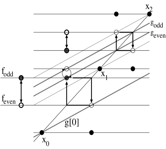
Figure 9: One of the simplest configurations for ‘type’ change. Type-I fixed points $x_{1},x_{2}$ and two type-II points generate a period-2 map (as in the upper-right square). A period-2 motion determined by the generated map generates a period-2 branch $g_{n}(x)$. Then, $g[0](x)$ and $g_{even}(x)$ produce a period-2 orbit (as in the lower left square). If the evolution of a point $f(x^{\prime})$ is determines by $g[0](x)$ ($g[even](x)$), $f(x^{\prime})$ is a type-III (IV) point. The sequence of the ‘type’ of $f(x^{\prime})$ is III, IV, III, IV, III, $\cdots$.

A simple example of the ‘type’ change is displayed in Fig.9. Here, fixed points in the right-hand part generate $g(x)$, which determines the dynamics of type-III point with period 2. The type-III points generate a time-dependent map that switches between $g_{odd}(x)$ and $g_{even}(x)$. The fixed points on the left-hand side generate $g[0](x)$, which determines the dynamics of the type-III points. Here, the fixed map consisting of $g[0](x)$ and $g_{even}(x)$ generates a period-2 orbit. If the evolution of the $f_{n}(x^{\prime})$ is determined by $g_{even}(x)$ at even $n$ or $g[0](x)$ at odd $n$, $f_{n}(x^{\prime})$ changes cyclically with period 2 as

$$\begin{array}[]{l}\left\{\begin{array}[]{ccl}f_{even}(x^{\prime})&=&g[0](f_{odd}(x^{\prime}))\\ f_{odd}(x^{\prime})&=&g_{even}(f_{even}(x^{\prime}))\end{array}\right.\end{array}$$ (12)

and its ‘type’ also changes cyclically with period 2 as III, IV, III, IV, $\cdots$. On the other hand, if the evolution of $f_{n}(x^{\prime})$ is determined by $g_{even}(x)$ at odd $n$ or $g[0](x)$ at even $n$, $f_{n}(x^{\prime})$ is a type-II fixed point.

When a type-III point possesses a chaotic orbit, as given in Sec.3.3, the nature of the functional dynamics determined by this type-III point is more interesting. Let us study the case with a chaotic generated map by constructing an example. By choosing a suitable initial function, one can embed a 1-dimensional map to construct a meta-map explicitly. For example, we adopt the following 1-dimensional map to be embedded:

$$\begin{array}[]{cc}x_{n+1}=2(1-\epsilon)x_{n}+\epsilon&(\bmod 1)\end{array}$$ (13)

This map has chaotic orbits for $\epsilon<1/2$. Indeed, the initial function $f_{0}(x)$

$$\begin{array}[]{l}f_{0}(x)=\left\{\begin{array}[]{cl}x&x\in[0,(1-\epsilon)/2],[(1+\epsilon)/2,1.0]\\ \frac{1-\epsilon}{\epsilon}x+(3\epsilon-1)/(2\epsilon)&x\in((1-\epsilon)/2,1/2]\\ \frac{1-\epsilon}{\epsilon}x-(1-\epsilon)/(2\epsilon)&x\in(1/2,(1+\epsilon)/2)\end{array}\right.\end{array}$$ (14)

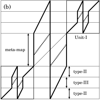
Figure 10: (a) A configuration (indicated by the solid line) which generates a map $x_{n+1}=2(1-\epsilon)x_{n}+\epsilon$ $(\bmod 1)$ (indicated by the dotted line) in the center square ($\epsilon=1/3$). (b) An initial function $f_{0}(x)$ leading to a hierarchical configuration of the map (a).

generates this map. In Fig.10(a), $f_{0}(x)$ is plotted for $\epsilon=1/3$. The dotted line represents a function $g_{0}(x)$ that has exactly the form $x_{n+1}=2(1-\epsilon)x_{n}+\epsilon$.

To construct a meta-map, we replace the type-I fixed interval in Fig.10(b) with this $f_{0}(x)$ (unit-I) by the transformation (5). With this nested structure, there are intervals where a type-III function exists, and the function generates an $n$-dependent $g_{n}(x)$ (CGM). This CGM acts as the map for a point that satisfies $f_{n}(x^{\prime})\in I^{1}\sqcup I^{2}\sqcup I^{3}$. For this configuration, the dynamics of a part of a CGM are determined by type-III points. In this case, a point which satisfies $f_{n}(x^{\prime})\subset I^{3}$ behaves as a type-IV point under the iteration.

In Figs.11(a)-(e), the evolutions of $f_{n}(x)$ and the meta-map are plotted, where the map $g_{n}(x)$ is plotted as a dotted line. Type-III points evolve according to $f_{n+1}(x^{\prime})=2(1-\epsilon)f_{n}(x^{\prime})+\epsilon$. In the present example, the slope $g^{\prime}(x)=2(1-\epsilon)$ is constant, and the slope of the type-III function $(f_{n}(x))$ is easily calculated as: $f^{\prime}_{n}(x)=\frac{(1-\epsilon)}{\epsilon}2^{n}(1-\epsilon)^{n}$. The generated map is determined as $g^{\prime}_{n}(x)=(1-\epsilon)+\epsilon f^{\prime}_{n}(x)$, and it has the form $g^{\prime}_{n}(x)=(1-\epsilon)\{1+2^{n}(1-\epsilon)^{n})\}$. Hence, this meta-map has a part where its gradient increases exponentially with $n$.

This implies that our functional dynamics can have stronger orbital instability than deterministic chaos: A tiny deviation $\delta$ from a point mapped to this type-III points grows as $\prod_{n=i}^{N}|g^{\prime}_{n}(x)|$. Since $\prod_{k=1}^{n}\alpha^{k}=\alpha^{\frac{n(n+1)}{2}}$, the leading order of the exponent of the orbital instability is $n^{2}$. Hence, the orbital instability is such that a tiny deviation grows as $exp(const\times n^{2})$ rather than $exp(const\times n)$, as is the case in conventional chaos. Due to this strong instability based on chaotic dynamics in the generated map, we call this dynamics ‘meta-chaos’. In Fig.11(f), an example of the orbits for meta-chaos is displayed. This evolution is determined by $g_{n}(x)$. The ‘type’ of the point changes between III and IV according to the map $g_{n}(x)$.

For a numerical simulation with this meta-chaos, the required mesh size increases as $2^{n}$. Hence, a simulation quickly becomes invalid as $n$ increases.

In the example mentioned above, we have constructed a meta-map by choosing special initial conditions. However, we note again that a meta-map configuration itself is not special and can be reached, for example, from a random initial function. Still, it is very rare to obtain a continuous type-I fixed interval from random initial conditions. Hence, in most simulations from arbitrarily chosen initial functions, we mostly observe generated maps of the Nagumo-Sato type, where magnitude of the slope, $|g_{n}^{\prime}(x)|$, is always less than 1.

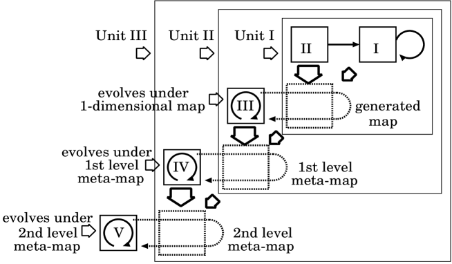
Figure 12: The schema of the meta-map. A 1-dimensional map can be generated from the configuration of type-I and II fixed points (unit-I). The function $f_{n}(x)$ iterated by this map is a type-III point which generates a meta-map (unit-II). The meta-map is determined by the map generated from a type-II fixed function and determines a dynamics of a type-IV point. The type-IV points and unit-II generate a higher level meta-map. This process can be continued recursively.

The nesting process of the meta-map can be continued hierarchically, since the configuration of type-I, II and III points, discussed above, can be a CS, which generates a CGM as a whole. This arrangement is called a ‘unit-II’. One can replace a unit-I in the above construction by such a unit-II. In such a situation, type-IV points generate a map, and with an appropriate configuration, the generated map can be a CGM. Now we can call this CGM a ‘unit-III’. This hierarchy to form a ‘unit-$N$’ can be continued for $N\rightarrow\infty$ (see Fig.12). To continue this nesting process, we define the ‘unit-$N$’ and the $N$-th level meta-map as follows.

A unit-$N$ is an interval $U^{N}$ which consists of type-I, II,$\ldots$, $N+1$ points and satisfies the condition $g(U^{N})\subset U^{N}$. A point $f_{n}(x^{\prime})\in U^{N}$ (with $x^{\prime}\not\in U^{N}$) evolves by the unit-$N$ and has a ‘type’ from I to $N+2$. We denote a function defined on an interval of type-$N$ points as $f^{N}_{n}(x)$ and the generated map from $f^{N}_{n}(x)$ as $g^{N}_{n}(x)$ (a fixed function is written $f(x)$ instead of $f^{II}(x)$). The functional equation rewritten in a recursive form with respect to the ‘type’ has the form

$$\left\{\begin{array}[]{cll}f^{N}_{n}(x)&=g^{N-1}_{n}(f^{N}_{n-1}(x))&x\in I^{N},f(x)\in I^{N-1}\\ g^{N}_{n}(x)&=(1-\epsilon)x+\epsilon f^{N}(x)&x\in I^{N}\end{array}\right.$$ (15)

The $N$-th level meta-map is defined as a CGM consisting of $g(I^{1}\sqcup I^{2}),g^{III}(I^{3}_{n}),\ldots,g^{N+2}(I^{N+2}_{n})$, where a 1-dimensional map generated from type-I and II points is called the ‘0-th level’ meta-map. All meta-maps depend on the fixed function $f(x)$ and are constructed recursively as $f(I^{1}\sqcup I^{2}),f^{III}(I^{3}_{n}),\ldots,f^{N}(I^{N}_{n})$. The whole interval $I$ can be written $I^{1}\sqcup I^{2}\sqcup I^{3}_{n}\sqcup\cdots\sqcup I^{N}_{n}\sqcup\cdots$. Here note that a ‘type’ greater than 2 can change in time, although each point has a finite maximal value of its ‘type’, depending on the initial configuration.

The $N$-th level meta-map is determined by the configuration of type-I, II, $\ldots,N+2$ points. It is important that each unit-$N$ and each branch are bounded. We can arbitrarily arrange any unit-$N$ and type-III, IV, $\ldots N+2$ points according to the branches. The configuration producing a meta-map characterizes a ‘syntax’ for each $x$. Each $x$ has a time evolution as a type. The ‘type’ of a point that is of type-III or higher changes in time. For a meta-map higher than second level, there is a sequence, for example, III, III, IV, V, III, $\ldots$. There is a transition relation among type-$N$ ($N>2$) points. Each point evolves under a hierarchy of meta-maps. In the above representation, the dynamics of the $N$-th level meta-map is independent of that of the type-$N+3$ points.

In a high level meta-map, the orbital instability is stronger than the exponential instability of conventional chaos. If $g^{\prime}(x)\sim\alpha$ $(|\alpha|>1)$ and $f^{III}_{i}(x)$ with a gradient $\beta$ is not a constant function (i.e., $\beta\neq 0$), then $f^{III\prime}_{n}(x)\sim\beta\prod_{k=i}^{n}\alpha\sim\alpha^{n}$, and $g^{III\prime}_{n}(x)\sim\alpha^{n}$. Now, the leading order of the slope of a 1st-level meta-map is $\alpha^{n}$, as is mentioned above. A type-IV function $f^{IV}_{n}(x)$ evolves under this 1st level meta-map. If $f^{IV}_{i}(x)$ is not a constant function and has a gradient $\gamma\neq 0$, $f^{IV\prime}_{n}(x)$ is calculated as $\gamma\prod_{k=i}^{n}\alpha^{k}\sim\alpha^{n^{2}}$, and $g^{IV\prime}_{n}(x)\sim\alpha^{n^{2}}$. Hence, $f^{V\prime}_{n}(x)\sim\alpha^{n^{3}}$ and $g^{V\prime}_{n}(x)\sim\alpha^{n^{3}}$. Repeating this argument, the leading order of the slope of the $N$-th level meta-map is given by $\alpha^{n^{N}}$. Thus a tiny deviation from a point, which evolves under the meta-map, is amplified by $|\alpha|^{n^{N}}$ at each $n$ step. Because of this, an $N$-th level meta map has an orbital instability that behaves as $exp(const\times n^{N+1})$. The level of the orbital instability increases with the level as $exp(const\times n^{N+1})$. In other words, an exponent $\lambda$ corresponding to the Lyapunov exponent of conventional chaos increases as $\lambda\sim n^{N}$ as $n$ increases for the $N$-th level meta-map.

5 Summary and Discussion

In the present paper, we have studied functional dynamics, focusing on the generation of rules (mappings) for the dynamics representing change of a function, and on the hierarchy of meta-rules.

As a first step, we introduced a new concept, the ‘generated map’ $g(x)$, which is derived from $f_{n}(x)$ and determines the dynamics of $f_{n}(x)$. The dynamics of some other parts of $x$ are determined by this generated map, while a closed generated map is defined as one that maps a region into itself. Functional values on some intervals were shown to change according to the generated map. This leads to a 1-dimensional map or a ‘meta-map’ that changes the map itself.

In Sec.3, we explicitly showed that some classes of 1-dimensional maps are embedded into this functional dynamics. In Sec.3.1 and 3.2, a piecewise linear map with two intervals of the slope $1-\epsilon$ were shown to be generated from two type-I fixed points and two intervals of corresponding type-II fixed points. Next, this construction was generalized to cover the case with several isolated type-I fixed points and the corresponding type-II intervals. There, a piecewise linear map with several intervals with slope $1-\epsilon$ were found to be generated. This map, called a ‘multi-branch Nagumo-Sato Map’ exhibits periodic cycles. Hence, the dynamics of the functional values determined by this generated map display a periodic cycle, which explains why periodic cycles are often generated in our functional dynamics.

In Sec.3.3, generated maps with continuous type-I fixed intervals and type-II points were discussed. In this case, a 1-dimensional map with an arbitrary slope can be embedded. Now, the functional dynamics determined by this generated map can also exhibit chaotic dynamics.

As shown in Sec.4, this construction of generated maps can continue hierarchically. The dynamics determined by a generated map forms a higher-level generated map that determines the dynamics of other regions. Since this map is changed by the first generated map, it is regarded as a ‘meta-map’, a map determined by another map. This procedure can be continued ad infinitum, leading to meta-meta-… maps. When a generated map exhibits chaotic dynamics, as discussed in Sec.3.3, the dynamics by meta-map can exhibit ‘meta-chaos’, in the sense that the evolution rule itself changes chaotically in time. It was shown that this meta-chaos has a stronger orbital instability than in chaos, in the sense that a small deviation is amplified as $exp(const\times n^{M+1}))$ for the $M$-th level meta-map, rather than $exp(const\times n)$.

Now, we discuss the relevance of our results for the target problems listed in Sec.1. The basic structure of the functional dynamics is provided by two types of fixed points, while a 1-dimensional map is generated by the configurations of fixed points. The evolution of the type-III points is determined by the map generated by several type-II intervals. A fixed point is invariant under iterations of the map and can be regarded as the basis (words) for the description of the world. The network of fixed points (word) generates the map $g(x)$ (rule). A set of orbits of type-III points can be regarded as the abstraction and categorization for the words. The words generate a rule, and the orbit determined by this rule determines a set of words. Thus, there is a circulation between words and rules, in the sense that the network of words generates a rule and that an orbit determined by the 1-dimensional map can be regarded as a representation of the operation on the fixed point (word).

Similarly, the 1st-level meta-map determines an orbit consisting of type-III and IV points, as an operation on a set of type-II and type-III points. In this hierarchical configuration, each orbit is characterized by a sequence of types and a sequence of values $f_{n}(x)$. A point, which evolves under the $N$th level meta-map, changes its “types’ variously, type-III, IV, $\ldots,N+3$. The sequence of ‘types’ determines the operation on elements which belong to various types in the hierarchy. This is regarded as a representation of the modality of a connection between words/rules and rules/meta-rules.

A map and a meta-map determine an orbit, which evolves following a lower level structure in the hierarchy. In our system, a higher-level structure is formed based on the lower-level structure, which we believe is an important characteristic in language. For example, syntax with regard to words is generated in our system, while this syntax depends on the words themselves. The ‘type’ of a word never changes in time, and the operation (orbit) on the words is determined by the time evolution.

The articulation as a whole is represented as $I=I^{1}\sqcup I^{2}\sqcup I^{3}_{n}\sqcup\cdots\sqcup I^{N}_{n}\sqcup\cdots$. The suffix $n$ is derived from the orbit of each ‘type’. A possible region where an orbit can exist is determined by a branch of the generated map, while the possible region where the branches can exist is determined by the orbit. The abstract language/object space is organized by the real orbit, which is one of the possible orbits under the restriction that of the partition $A_{n}=\sqcup_{i}\{I^{i}_{n}\}$.

When a partition $A_{n}$ is given, an infinite variety of possible orbits can exist. Depending on the evolution, a different $A_{n+1}$ can be formed. The syntax given by the partition $A_{n}$ crucially depends on the orbit, which on the other hand is determined by the generated map organized through $A_{n}$. The syntax (i.e., the rule derived from the generated maps) and the semantics (i.e, the orbit of functional dynamics) determine each other, and cannot be derived independently. This situation can be regarded as representing the ‘speech act’, in which syntactic structure (a generated map) generates an utterance (orbit), and the utterance changes the syntactic structure.

In formal language theory, a grammar is implemented independent of semantics, as an innate structure. In our functional dynamics, such rules governing the use of words are thought of as being formed only through iterations. No other assumption except for the choice of non-trivial initial functions is required. Since iterations are essential to language, we expect that the formation of rules in our system, depending on words themselves, is relevant to the origin of syntax and semantics in language.

In our system, a hierarchical structure is also formed through iterations. This hierarchy is also a characteristic of language, and it is important to note that a simple class of functional dynamics with recursive structure can provide such hierarchy in general. The hierarchical structure in this system has a strong dependence on the lower-level structure, since the higher-level structure is determined according to which branch of the generated map is taken by the orbit.

The form of the generated map $g(x)$ depends on the configuration of type-I fixed points. If they are discrete, the slope of $g(x)$ is smaller than 1. When there exists a continuous interval of fixed points, $g_{n}(x)$ can have a slope larger than 1, and the meta-map can have a more complex orbit than in chaos. A continuous type-I fixed interval is generated by an identity function over some interval, which corresponds to a filter with which an agent acts in response to the world without interpretation. In other words, chaotic functional dynamics and meta-chaos are generated by adding a continuous input from the external world to the ‘closed’ world of functional dynamics only with self-reference.

Possible extensions of the present study will be discussed in the future. In a 2-dimensional version of the functional dynamics, an arbitrary 2-dimensional map can be embedded in the same way as in Sec.3.3. Because of this, we can embed a Turing machine into this system [9] (see also Appendix B), where the search for a relationship between the generalized shift [9] and meta-dynamics (meta-chaos) will be important.

Non-trivial sets of functions over functions are studied in domain theory [10] [6] [7]. The most important difference between systems studied in domain theory and our model lies in the dynamical aspects of functions treated only in our approach. However, our meta-map is restricted within some intervals and is not extended over the whole domain. Indeed, in our system the size of the $N$-th level meta-map decreases with order $\epsilon^{N}$. However, such a contraction can be removed in a more general functional dynamics. This will be important to obtain functional dynamics allowing for a hierarchy of the meta-map over the whole domain.

Another extension required for language will be the inclusion of dialogue [2]. To this point, we have only considered one agent whose function changes recursively. To study the social structure of language, functional dynamics with several agents is necessary.

Appendix A Some Properties of $F(x,y)$

In this appendix, we investigate a general class of functional maps with the form

$$f_{n+1}(x)=F(f_{n}(x),f_{n}\circ f_{n}(x)).$$ (16)

We study a fixed point condition and properties of the generated map.

This type of functional equation has fixed points (fixed functions). First, we define $Z(x)$ from $F(x,y)$. Here, $Z(x)$ is the solution of $x=F(x,Z(x))$. The fixed point condition is defined from $Z(x)$. If the condition $f\circ f(x^{\prime})=Z(f(x^{\prime}))$ is satisfied, $f(x^{\prime})$ is a fixed point. If $F(x,y)=(1-\epsilon)x+\epsilon y$, then $Z(x)=x$, and the fixed point condition is nothing but $f\circ f(x^{\prime})=f(x^{\prime})$. The fixed point condition in the present general case is determined as follows. (We give the correspondent equation for the case with $F(x,y)=(1-\epsilon)x+\epsilon y$ in the square bracket $[...]$, for reference.)

(i)

If $Z(x)$ is a single valued function, $f(x)=Z(x)$ is a fixed function over the entire interval ($f\circ f(x^{\prime})=Z(f(x^{\prime})$).

[$f(x)=x$ is a fixed function]

(ii)

The point where $Z(x)$ intersects the identity function ($x^{\prime}=Z(x^{\prime})=f(x^{\prime})$) is a fixed point ($f\circ f(x^{\prime})=f(x^{\prime})=Z(x^{\prime})=Z(f(x^{\prime}))$).

[Type-I fixed point condition]

(iii)

If a point $(x^{\prime},f(x^{\prime}))$ is a fixed point ($f(x^{\prime})=Z(x^{\prime})$), a point $(x^{\prime\prime},f(x^{\prime\prime}))$ which satisfies $f(x^{\prime\prime})=Z(x^{\prime\prime})=x^{\prime}$ is also a fixed point ($f\circ f(x^{\prime\prime})=f(x^{\prime})=Z(x^{\prime})=Z(f(x^{\prime\prime}))$).

[There is no such fixed point corresponding to this case]

(iv)

If a point $(x^{\prime},f(x^{\prime}))$ is a fixed point, a point $x^{\prime\prime}$ with $f(x^{\prime\prime})=f(x^{\prime}))$ is also a fixed point.

[type-II fixed point]

The most noteworthy difference from the case with $F(x,y)=(1-\epsilon)x+\epsilon y$ is seen in (iii). For a point $f(x^{\prime\prime})=Z(x^{\prime\prime})$, the fixed point condition is that $Z\circ Z(x^{\prime})$ is a fixed point. There, $Z(x)$ decides a fixed point condition as an orbit of a 1-dimensional map. In other words, the ‘attractor’ of $Z(x)$ is a fixed point of the equation (15), and a sequence $\{f(x^{\prime}),Z\circ f(x^{\prime})=f(f(x^{\prime})),Z^{2}\circ f(x^{\prime})=f(Z\circ f(x^{\prime})),\ldots,Z^{\infty}\circ f(x^{\prime})\in$ attractor $\}$ consists of fixed points.

The functional equation can be divided into

$$\left\{\begin{array}[]{lcl}f_{n+1}(x)&=&g_{n}\circ f_{n}(x)\\ g_{n}(x)&=&F(x,f_{n}(x))\end{array}\right.$$ (17)

as in the case $F(x,y)=(1-\epsilon)x+\epsilon y$. The generated map viewpoint is also effective in this general case.

However, for a general $F(x,y)$, the transformation (5) cannot be adopted, because $F(x,y)$ is not linear. However, the use of a generated map to construct a meta-map remains valid in a general $F(x,y)$ case, and a hierarchical configuration can exist for a particular configuration.

Appendix B Multi-Branch Nagumo-Sato Map

In general, $f(x)$ with (at least) two type-I fixed points has the potential of possessing a Nagumo-Sato map as a generated map. To consider the general situation, we define the ‘multi-branch Nagumo-Sato map’ by (6), restricted within a region $I=[x_{0},x_{n-1}]$, while $x_{0},x_{1},\ldots x_{n-1}$ can be arranged arbitrarily. This type of map can be generated from random initial conditions.

In this map, we can choose a function which generates a map producing cycle of any length of period. To illustrate this property, we study the case with some special configurations.

First, two type-I fixed points are assumed to be 0 and 1. For the sake of symmetry, we choose $\epsilon=1/2$. Then, the two branches are given by

$$\left\{\begin{array}[]{clc}g[0](x)&=\frac{1}{2}x&x\in I^{2}_{0},f(I^{2}_{0})=0\\ g[1](x)&=\frac{1}{2}x+\frac{1}{2}&x\in I^{2}_{1},f(I^{2}_{1})=1\end{array}\right.$$ (18)

We represent a rational number $a$ by the binary form $0.a_{1}a_{2}a_{3}\cdots$, with each $a_{i}=0,1$ (here $a=\sum_{k=1}^{\infty}a_{k}2^{-k}$). In this representation, $g_{0}(x)$ acts as a right-shift, which acts as $0.a_{1}a_{2}a_{3}\cdots\rightarrow 0.0a_{1}a_{2}a_{3}\cdots$, and $g_{1}(x)$ acts as a right-shift and inserts 1 into the head of the sequence as $0.a_{1}a_{2}a_{3}\cdots\rightarrow 0.1a_{1}a_{2}a_{3}\cdots$. Hence these two branches act as 0, 1-inserter for a binary sequence.

Here we denote $a$ $(a_{i}=a_{i+m})$ as $\{a_{1}a_{2}\cdots a_{m}\}$, while the set of $m$-length sequences $\{a_{1}a_{2}\cdots a_{m}\}$ is denoted by $S_{m}$. The number of elements which belong to $S_{m}$ is $2^{m-1}$, and the values of $a$ $(\in S_{m})$ take $i/2^{m-1}$ ($i=0,1,\ldots,2^{m-1}$). If $\{a_{1}a_{2}\cdots a_{m}\}\in S_{m}$, $\{a_{m},a_{1}a_{2}\cdots a_{m-1}\}\in S_{m}$. Because of this, when $g(\{a_{1}a_{2}\cdots a_{m}\})\equiv g_{a_{m}}(\{a_{1}a_{2}\cdots a_{m}\})$, the map $g(x)$ is a bijection $S_{m}\rightarrow S_{m}$. We define $M_{m}(x)=g(x)$ over $S_{m}$.

$M_{m}(x)\cup M_{n}(x)$ is a single-valued function for arbitrary $m,n$. The condition that a point $a\in S_{m}\cap S_{n}(m<n)$ exists is that $m$ is a divisor of $n$. In such a case, $a$ has the form $\{a_{1}a_{2}\cdots a_{m}\}\in S_{m}$, and $\{a_{1}a_{2}\cdots a_{m}\}^{n/m}\in S_{n}$. These two representations determine the same $g(a)$. Then, $M_{\infty}(x)$ defined as $\cup_{k=1}^{\infty}M_{k}(x)$ has an infinite period.

The function $M_{m}(x)$ is defined at $2^{m-1}$ points. With an appropriate arrangement, it is possible for $g(x)$ generated by the attractor of our functional dynamics to be made equal to $M_{m}(x)$ for all $x$. As an example, we define g(x) as $g_{o(i)}$ for an interval $[i/2^{m-1},i+1/2^{m-1})$ $(i=0,1,\cdots 2^{m-1}-1)$. Here, $o(i)=0$ for even $i$ and $o(i)=1$ for odd $i$. In Fig.13, we can take a section_i $[i/2^{m-1},(i+1)/2^{m-1})\times[g(i/2^{m-1}),g(i/2^{m-1})+1/2^{m-1})$ within the region where $g(x)$ is defined. The map $g(x)$ determines the bijection section${}_{i}\rightarrow$ section_j. In each section, $g(x)$ has a slope 1/2 ($<1$), and all orbits converge to attractors which are determined by $M_{m}(x)$. Thus we can embed a multi-branch Nagumo-Sato map which has multiple attractors.

In the same way, we can construct an $n$-branch Nagumo-Sato map. We assume $x_{i}=i/n$ $i=0,1,\ldots,n-1$. If $\epsilon=(n-1)/n$, each branch has the form

$$g[i](x)=\frac{1}{n}x+\frac{i}{n}(x\in I^{2}_{i},f(I^{2}_{i})=\frac{i}{n})$$ (19)

Each branch $g[i](x)$ indicates a right-shift and insertion of $i$ at the head of the $n$-digit sequence. Using these branches, we can embed an $m$-periodic point for an $n$-digit representation $\{a_{0},a_{1},\ldots,a_{m-1}\}$ $(a_{i}=0,1,\ldots,n-1)$.

Appendix C Embedding a General One-Dimensional Map as a Generated Map

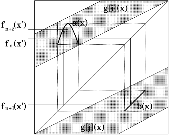
Figure 14: An example with an arbitrary 1-dimensional map embedded. Once the map is generated as in this figure, $f_{n}(x^{\prime})$, which takes a value in this region, evolves according to $f_{2n+1}(x^{\prime})=a(f_{2n}(x^{\prime}))$ and $f_{2n+2}(x^{\prime})=b(f_{2n+1}(x^{\prime}))=b\circ a(f_{2n}(x^{\prime}))$. If $b(x)$ is the identity function, $f_{2n+2}(x^{\prime})=a(f_{2n}(x^{\prime}))$. An arbitrary 1-dimensional map can be embedded by observing the dynamics of the function every two steps.

Let us examine closely the configuration of the type-I fixed intervals adopted to embed a 1-dimensional map. The area in which a 1-dimensional map is embedded has to be on the intersection between each branch of type-II intervals and $I\times\bar{I}^{1}_{i}$ (See.Fig.6). This implies that we cannot embed a map which is continuous around the identity function. However, one can embed an arbitrary 1-dimensional map by considering a two-step iteration, i.e., as a map to generate $f_{n+2}(x)$ from $f_{n}(x)$. As shown in Fig.14, let us take two maps in the dotted areas of Fig.6. As shown in the figure, the generated maps $g[0](x)$ and $g[1](x)$ are put in two regular square sections. Here, $f_{n}(x^{\prime})$ which is mapped to $g[0](x)$ evolves as $f_{n+1}(x^{\prime})=g[0](f_{n}(x^{\prime}))$ and $f_{n+2}(x^{\prime})=g[1]\circ g[0](f_{n}(x^{\prime}))$. If $g[0](x)$ is the identity function, the time evolution of $f_{n}(x^{\prime})$ at $n=2i$ ($i$ integer) is $f_{n+2}(x^{\prime})=g[1](f_{n}(x^{\prime}))$, $f_{n+4}(x^{\prime})=g[1](f_{n+2}(x^{\prime}))$ $f_{n+2i}=a^{i}(f_{n}(x^{\prime}))$. Hence an arbitrary 1-dimensional map can be embedded as a rule for the two-step iteration of the functional dynamics.

Acknowledgments

The authors would like to thank Drs. T. Ikegami and S. Sasa for stimulating discussions. This work is partially supported by Grant-in-Aids for Scientific Research from the Ministry of Education, Science and Culture of Japan. One of authors (NK) is supported by a research fellowship from Japan Society for the Promotion of Science.

Figure 3: The schema of the generated map. The configuration of type-I and type-II fixed points generates the map, while the evolution of the type-III points are determined by the generated map.

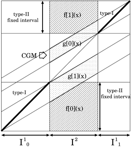
Figure 6: The closed 1-dimensional map. Using two type-I fixed intervals, we can obtain a larger class of a 1-dimensional map. The type-II fixed function $f(x)$ is represented by $f[0](x)$ (for $x\in I^{1}_{0}$) and $f[1](x)$ (for $x\in I^{1}_{1}$). $I^{2}$ is a domain of the type-II fixed function $f(x)$. The generated map $g(x)$ is given by $g[0](x)=(1-\epsilon)x+\epsilon f_{0}(x)$ (for $x\in I^{1}_{0})$ and $g[1](x)=(1-\epsilon)x+\epsilon f_{1}(x)$ (for $x\in I^{1}_{1})$. We call this type CGM a ‘unit-I’. In this figure $\epsilon=0.5$.

Figure 11: Time evolution of $f_{n}(x)$ and $g_{n}(x)$. (a) $f_{1}(x)$ (solid line) and $g_{1}(x)$ (dotted line). (b) $n=2$. (c) $n=3$ (d) $n=10$ (e) $n=11$ (f) Time evolution of one point $f(x^{\prime})$, determined by the generated meta-map, at the center square ($0<x<200$). The ‘type’ of the function $f_{n}(x^{\prime})$ changes between III and IV in time. Squares indicate that the ‘type’ of $f_{n}(x^{\prime})$ is IV at $n$. Since the mesh size required for the computation is extremely large, the plotted orbit is not precise. It is expected, however, that the statistical properties are conserved with this numerical computation.

Figure 13: A multi-branch Nagumo-Sato map $M_{3}(x)$. Two period-3 attractors coexist.

References

- [1] N. Kataoka, K. Kaneko, ”Functional Dynamics : I Articulation process” submitted to Physica D
- [2] N. Kataoka, K. Kaneko, ”Functional Dynamics : III : Dialogue and Community” in preparation
- [3] N. Kataoka, K. Kaneko, ”Functional Dynamics for Natural Language” submitted to Biosystems
- [4] N. Chomsky, ”On certain formal properties of grammar” Information and Control 2, 393-395, 1959
- [5] J. E. Hopcroft, J. D. Ullman, ”Introduction to Automata Theory, Languages, and Computation” Welsley Pub Co, 1979
- [6] J. Soto-Andrade, F. J. Varela, ”Self-Reference and Fixed Points: A Discussion and an Extension of Lawvere’s Theorem” Acta Applicandae Mathmaticae 2, 1-19.
- [7] R. Rosen. ”Life Itself : A Comprehensive Inquiry into the Nature, Origin, and Fabrication of Life” Columbia U.P.,1991
- [8] J. Nagumo, S. Sato, ”On a Response Characteristic of a Mathematical Neuron Model” Kybernetik 10 (1972) 155-164
- [9] C. Moore, ”Generalized Shifts : unpredictability and undecidability in dynamical systems” Nonlinearity 4 (1991) 199-230
- [10] G. D. Plotkin, ”Domains” Unpublished lecture notes, Dept. Computer Science, University of Edinburgh, 1983