Functional Dynamics I:
Articulation Process

Abstract

The articulation process of dynamical networks is studied with a functional map, a minimal model for the dynamic change of relationships through iteration. The model is a dynamical system of a function $f$, not of variables, having a self-reference term $f\circ f$, introduced by recalling that operation in a biological system is often applied to itself, as is typically seen in rules in the natural language or genes. Starting from an inarticulate network, two types of fixed points are formed as an invariant structure with iterations. The function is folded with time, until it has finite or infinite piecewise-flat segments of fixed points, regarded as articulation. For an initial logistic map, attracted functions are classified into step, folded step, fractal, and random phases, according to the degree of folding. Oscillatory dynamics are also found, where function values are mapped to several fixed points periodically. The significance of our results to prototype categorization in language is discussed.

submitted to Physica D

1 General Introduction

In studying a biological system, we face the problem of how rules are generated. In simulations of physical systems, a rule is given in advance from a natural law. On the other hand, in trying to model a biological system at a biological level, we need to study the origin or dynamics of the rule itself.

There are two possibilities for such a study. In one approach, one starts from a level that is more microscopic than that of the biological system (e.g., the chemical reaction level) and determines form a description of of behavior on this smaller scale how a rule (e.g., a rule for cell differentiation) is formed at a biological level. In the other approach, one attempts to start at a biological level from the beginning.

Since the latter approach, when successful, can allow for the extraction of the essential features of a biological system, we consider this approach here. In attempting to employ this approach, however, we face the following difficulty. In this approach, the rule (operator) and variable (operand) are not initially distinguished, and they should be at the same level in the beginning. For example, consider a gene. This is nothing but a set of chemicals within a DNA molecule. Among the chemicals in a cell, the chemicals contained in the DNA molecule constitute some kind of ‘rules’ for other chemicals. A more straightforward example is seen in the problem of language, where code and encoding are not distinguished at a descriptive level. If a language were nothing but a signal (as is the case for the emergency calls of birds), there would be no need to distinguish code from encoding. However, it is thought that there is something called ‘encoding’ within our language. In spite of the conviction that there is meaning in an uttered phrase or piece of text, this meaning can be described only at the code level. Although in describing encoding, it is represented by a set of codes, the encoding in the natural language needs something beyond such a set. (See Sec.2 for discussion on language.)

In view of the above considerations, it would seem that we need to construct a model in which the rule (operator) is not initially separated from the variable (operand). In the case of language, we have to start from a model without distinction between code and encoding. Since a rule is not distinguished from the entity to which the rule is applied, the operation of a rule can be applied to itself. Hence, one has to consider ‘self-reference’ seriously. As will be seen, we consider the dynamics of networks of relationships. These dynamics are formulated in terms of the dynamics of function, instead of dynamics of variables. In this formulation, self-reference is expressed by the operation of the function on itself (i.e., $f\circ f(x)$).

The second problem in a biological system is the emergence of symbols, made possible by ‘articulation’ of continuous objects. Here, ‘articulation’ means the categorization of the words or molecules. Although this categorization is usually used as a classification of some elements at the same level into some groups, the inseparability of the rule and the variable has to be considered, as pointed out in the discussion of the first problem. Thus, the articulation is used to describe a categorization of words and rules. Through the dynamics of networks of relationships of objects, some object begin to act as a symbolization of other objects. This can be seen in the emergence of ‘information carrying molecules’, such as DNA, and in the emergence of language with some symbols. Once the symbols are formed, they remain as stable objects, while connections to such symbols are formed as relatively stable relationships. In the present paper, the process of articulation is studied through the dynamics of functions.

The third problem in the study of a biological system is understanding the formulation of a rule to change the relationships among objects. Such a rule leads to dynamics of the symbols, but it also refers to the object assigned to the symbol. For example, rules for differentiation are formed in reference to genes (symbols) in DNA, but these rules also can depend on other chemicals associated with the genes. Although grammar consists of rules concerning symbols, often these rules are not completely syntactic, but rather depend on the objects that are assigned to symbols.

The fourth problem is that of hierarchical rule formation, as is seen in the development process of an organism or in the language. Here the dynamics of the changes of the rule itself emerge as a meta-rule.

The fifth problem is understanding the formation of a ‘social’ rule among some subjective, tissues or organs. The ‘society’ of ‘units’ is assumed to have a common rule. On one hand, this rule is given from the form of the whole society, and on the other hand, it is generated from the concurrence among some units.

In a series of papers, we attempt to construct a mathematical framework that solves the above five requisites. In this, the first paper of the series, we consider the basic structure of the functional map, and discuss the articulation process. The third and fourth problems, which are more central to the present formulation, will be discussed in the next paper. The fifth problem will be discussed in a third paper.

2 Introduction

Before discussing our model and the results of articulation dynamics, we briefly mention our motivation in connection with the study of language. Since some epistemological understanding are necessary to study natural language, we briefly review trends in the philosophy of language.

Although a logical model for language was extensively studied from the 1920s to the 1950s in the context of ‘logical positivism’ [1][2], this approach could not cover the entire area of cognition or semantics. Theory-laden nature of measurement [3] and the position of the real world in the theory then led to a shift from ‘logical positivism’ to ‘logical negativism’ [4]. There, it has been recognized that a theory of natural language is not sufficient without the concept of cognition. By this recognition, new trend in the language theory started, that is the theory of the ‘speech act’ (usage of language), which focuses on ‘intention’ [5][6]. This theory, however, is grossly insufficient given the diversity of utterances. In the logic-based theory, the problem of how the continuous world can be represented by combinations of finite words is not addressed. In the theory, only minimal elements and rules governing these elements from the outset are included.

In contrast to the above theories, ‘structurism’ attempts to attack the background of language [7]. It the structurism, one focuses on how continuous objects are articulated into words, depending on the structure of all other words. However, this theory deals only with ’static’ structure, and can only describe a ‘snapshot’ property of the language mechanism, which indeed has developed from each individual’s birth and evolved historically since its origin. There are some philosophical discussions [9] with regard to replacing a theory of the static structure of language by a theory including dynamics, but these remain speculative, without any concrete mathematics. A mathematical model for epistemology or articulation dynamics is necessary to study natural languages. However, in a mathematical model we cannot deal with cognition directly. Thus, a ‘detour’ is needed to understand the underlying basic structure of languages.

Since phones and letters are only signs, it is not possible to distinguish a code from the encoding entity. There is only a circulation of signs. The code-encoding relation is decided by correspondence to the real world, although the dynamics of signs seems to be self-driven at the descriptive level, too.

The dependence of the rules imposed on signs upon the description level is evidenced by the existence of dictionaries. This existence implies that a sentence cannot be produced only from the formal logic. If all sentences were made logically, dictionaries would be much thinner or perhaps would be unnecessary. The role of dictionaries shoulder the redundancy in language, which is beyond the formal logic. This redundancy is related to cognition and derives from the uniqueness of our world. Hence, this redundancy shown by the existence of dictionary has to be considered seriously for the study of cognition. In addition to redundancy, an important characteristic of dictionaries is the circulation among words. A word is described by other words, which are, in turn, described by still other words. In other words, there are self-referential relations among signs. This self-referential structure is taken into account for our ‘detour’ of understanding the basic structure of language systems.

However, if we focus only on the static network of words, the detour is not relevant to the study of cognition. The static network that has already been articulated is only a snapshot of language. To study the static structure of language, we need a database of existing languages, which we cannot include in our preliminary study with an abstract mathematical model. Rather, in our study, we focus on some universal structure that the articulation in dynamical networks possesses, from which we regard the articulation process of cognition as one important aspect of the natural language. Of course, this is a difficult problem that cannot be solved in a single paper. Here we present a first attempt at solving this problem by introducing an abstract model for a dynamical network and study a class of general phenomena.

In previous studies of natural language, it is common for code and encoding to be divided. The celebrated theory of code is the ‘generative grammar’ (Chomsky 1955) [8], while ‘cognitive semantics’ (Lakoff 1987) [10] is a theory for the encoding.

For the study of codes, generative grammar deals with transformation of words and sentences. Given a formal system, such transformations are classified into several classes [11], according to computation theory. Study of generative grammar has succeeded in describing how an already described language is structured. However, this is just a one-way flow from the phones or letters to the language structure. Natural language cannot be generated only by this language structure. To produce a sentence, it is inevitably necessary to refer to the real world. If we have to refer to real world structure in order to produce sentences, the syntactic rules must be complemented by additional cognitive rules in order for a machine to be able to speak or a program to be able to write. Thus, a theory or a model of articulation of language is necessary, for example, to construct a machine which can use language.

In this respect, cognitive semantics deals with the structure of the linguistic network among words, which is preserved and constructed through the iteration. It is proposed that there is semantic structure (a network of category, or a set of sets of words), which is formed through these iterations and is robust to some degree. This semantic structure is an articulation of the real world. Although a category is a set of words, it is not decided only from properties of objects, but also through cognitive processes. Because of this property of a category, it is not the case that all the words in the category have the same status, and thus there is asymmetry in the structure of the category derived from cognition. A reference element which is suitable for the cognitive process (restricted physically, socially and so on) is called a ‘prototype’ [10], while other elements in the same category can have various status. The repeated use of language produces a semantic network of category whose prototype is essential to the articulation in the language.

In communication it is essential that some entities are identified through iteration which is restricted, for example, by cognitive, physical, social and common laws. Iteration gives the foundation of the language. If the language were not formed through iteration, it would be destroyed into fragments like those Borges imagined [12] or in Finnegans Wake. Some iteration processes preserve meaning, while some others alter existing meanings. With the confliction of these two processes, one can describe something already described, while one can also think about what has not yet been described. By iterating encoded words in a language network, such a network is formed as a connection of codes.

A fuzzy logic can be one of the tools to extract semantic structure, because each element which belongs to the category can have a different status. However, semantic structure formed through the cognitive process has a dynamical aspect, and hence a fuzzy ‘logic’ is not sufficient to deal with it. To consider cognitive and semantic processes, a dynamical model of fuzzy logic [13] and a dynamical network of proposition in a fuzzy logic as a functional form [14] have been proposed. However, to study the duality between rule and code directly, we must avoid such a logic-based approach. Starting from an inarticulate system without logic, the emergence of articulation is studied in this paper, while the emergence of rule (logic) is studied in the next paper, II.

To sum up the long discussion so far, we have to study a system having following features: (a) networks of relationships change in time, (b) rules (operators) and variables (operands) are not initially separated (c) the rules (operators) are applied to themselves, since operands are not separated (d) through the iteration of the rules (e.g., the use of language), some robust structure in the network is formed, by which the roles of operators (rules) and operands are separated (e) from continuous objects, discrete symbols are formed through the iteration of the rules to change the network of relationships.

To represent an inarticulate network mathematically, we adopt a function (network) instead of a variable, as its minimal element (word). This function $x\rightarrow f(x)$ can represent the network of relationship, or a filter from inputs to outputs. With this representation by a function, the application of a rule to itself is represented by the self-reference term $f\circ f(x)$ so that the relationship $x\rightarrow f(x)$ is applied to $f(x)$ itself. Since the operand of the function is the function itself in this term, the operator and operands are not separated.

In addition to the robust structure with respect to iteration, the language has ability to create variety. Objects indicated by codes can vary in context and in time. Also, if a novel object, which has not existed before, appears, language is able to refer to it. Conversely, we can describe only what our language can approach. In spite of this restriction, we can always face new objects in a new manner. Hence the network structure in language has variability to support such diversity. To cope with such variability, a dynamics of the function $f(x)$ will be introduced into our model, so that the relationship $x\rightarrow f(x)$ can change dynamically. We study the evolution of the function $f_{n}(x)$ at time step $n$, following functional dynamics depending on $f_{n}(x)$ and $f_{n}\circ f_{n}(x)$.

By taking a continuous variable $x$, the problem of articulation will be studied as a classification process how $f_{n}(x)$ converges to distinct intervals in each of which $f_{n}(x)$ takes a different constant value. For a given value $a=f_{n}(x)$ the inverse set $I_{n}=f^{-1}_{n}(a)$ is given as an articulated class. This means that the filter articulates the continuous world $x$ into some segments according to the value $f_{n}(x)$.

This paper is organized as follows. We propose a model of the articulation process in Sec.3, where a map for a function $f(x)$, not for a variable $x$, is introduced. The dynamics of this function are given by a balance between the original map $f(x)$ and its iteration $f\circ f(x)$. As a preliminary step for later studies, we discuss some elementary properties of these functional dynamics in Secs.4 and 5. In Sec.4, we discuss the case in which the dynamics are given only by $f\circ f(x)$, to clarify periodic dynamics of the network. In Sec.5, we discuss the simplest case with a monotonic function, to understand the minimal articulation property of our dynamics. In Sec.6 we choose a single-humped map as an initial function, to understand the articulation process balancing between self-reference and diversity. The limiting forms of the functions are classified in Secs.7 and 8 by introducing several quantities characterizing stepwise, fractal and other singular functions. A self-folding mechanism is discussed in detail. Periodic solutions in this model are given in Sec.9. Summary and discussion are given in Secs.10 and 11.

The possible class of behavior in our functional dynamics is not restricted to those discussed in the present paper. Here, we discuss only periodic structures generated by isolated fixed points. Indeed, a method to determine periodic points mapped to continuous fixed points is presented in a subsequent paper, where hierarchical rules to change rules will be organized in our functional dynamics [15].

3 The Model

As a minimal model of the dynamics of articulation or categorization, we introduce a functional dynamics. Here a function represents a relation among elements that can be words, chemicals, and so forth. In this abstract model, a function corresponds to a network consisting of directed elements. We study some characteristic features of functional dynamics with the iterated application of the function to itself.

Given an initial network, it evolves according to a transformation rule that is determined by the shape of the network itself. On one hand, the function is postulated to have a self-referential property through the operation of the function on itself. On the other hand, the function is required to have the ability to exhibit diverse behavior, to drive the network to include a variety of elements.

Here, we consider a minimal model with a transformation rule possessing both a self-referential structure and some driving mechanism leading to diversity. For simplicity, we restrict the initial network to that represented by a one-dimensional map, i.e., a one-variable function. This means that each point $x^{\prime}$ is mapped to a point $f(x^{\prime})$. In other words, the function $f(x)$ represents the connection between a point in the inarticulate network $x$ and another point $f(x)$. The function $f(x)$ determines a network of relations among words. By setting some initial relations through an initial function, we study how the network spontaneously grows and generates articulation from the initial inarticulate network. As the dynamics of the network, we postulate that the form of the function changes through reference to the function itself. This self-reference is represented by the application of the function to itself, given by the term $f\circ f(x)$. Another and equivalent possible interpretation may be made by regarding the function $f(x)$ as a filter from the input $x$ to the output $f(x)$. In a biological system, the filter is changed in time by some feedback process from its output. We try to capture the nature of the self-feedback process due to the output and its influence on the filter itself, as the simplest form of self-reference. Now the evolution of the function is written as follows:

$$f_{n+1}(x)=F(f_{n}(x),f_{n}\circ f_{n}(x)).$$ (1)

The term $f_{n}\circ f_{n}(x)$ changes the connections from $x\rightarrow f(x)$ to $x\rightarrow f\circ f(x)$ for all $x$. Next, we assume that the change of $f(x)$ vanishes when the self-reference of a function agrees with the function itself. In other words, we assume that the function can ‘relax’ to a fixed point function satisfying $f(x)=f\circ f(x)$.

For example, when one listens to a sound $x^{\prime}$ through the filter $f_{n}(x)$ and pronounces $f_{n}(x^{\prime})$, it is referred as $f_{n}\circ f_{n}(x^{\prime})$. In this case, the relation $f(x^{\prime})=f\circ f(x^{\prime})$ represents a self-consistent relation for the imitation of sound. If $f(x)=f\circ f(x)$ is satisfied as a whole function, the network is articulated to form a consistent input-output table.

As the simplest form of the evolution, we choose the form

$$F(x,y)=(1-\epsilon)x+\epsilon y,$$ (2)

which is nothing but the operation of a weighted mean with weight parameter $\epsilon$. The evolution equation of the function is now given by

$$f_{n+1}(x)=(1-\epsilon)f_{n}(x)+\epsilon f_{n}\circ f_{n}(x).$$ (3)

The time evolution of these functional dynamics is determined by giving an initial function $f_{0}(x)$ and a control parameter $\epsilon$. In other words, the inarticulate network spontaneously evolves without referring to the outer world. The outer world is given as an initial function $f_{0}(x)$. The complexity of the outer world ($f_{0}(x)$) and the intensity of self-reference $\epsilon$ determines the time evolution.

Although we have introduced the evolution rule of the function $f_{n}(x)$ as Eq.(3), this rule is applied within the functional space. We can study how some points $f_{n}(x^{\prime})$ work as rules for other points, through the application of the function to itself by (3). Indeed, the emergence of rules from objects will be demonstrated in a subsequent paper.

Depending on the initial function $f_{0}(x)$, the final state of the function as $n\rightarrow\infty$ is generally different. These different $f_{n}(x)$ represent the variety of manners of articulation as a network of relations. Here we study the evolution of the function under this iteration, varying the initial function $f_{0}(x)$ and the (control) parameter $\epsilon$. In the present paper, we choose a monotonically increasing function, a logistic map (as a representative of single-humped map), as the initial function $f_{0}(x)$, while some other $f_{0}(x)$ leading to periodic points will be briefly discussed in Sec.9.

A model related to with ours, including the $f\circ f$ term, was proposed by Deutsch [16] [17]. In that model motion in a random potential is studied under the iteration of functions.

4 Recursive Equation with $\epsilon=1$

First, we discuss the case $\epsilon=1$, in which the dynamics of the network are simple. The equation is written

$$f_{n+1}(x)=f_{n}\circ f_{n}(x).$$ (4)

This iteration yields snapshots of $2^{n}$ steps of the equation $g_{n+1}(x)=f_{0}(g_{n}(x))$, $g_{0}(x)=x$. If $f_{0}(x)$ is a map which generates a chaotic orbit, equation (4) generates a chaotic sequence.

As a simple introduction, let us consider the ‘discrete mesh’ case, where the initial function $f_{0}(x)$ takes only $M$ possible values, (for example given by $f(i)=j$ $(i,j=0,\ldots,M-1)$. We adopt the integer index $i$ for each element in this discrete mesh, and we denote by $f(i)$ the functional value at $i$. In this case, we can consider only $M$ elements, and the function is nothing but a network from $[0,1,\ldots,M-1]$ to the same set. Once a map, represented by a finite mesh, is given, the model gives the dynamics of the network in which each element connects to itself or to a different element. Each element is represented by a site index $i$, while $f_{n}(i)$ gives the site index to which $i$ is mapped.

In this equation, the functional map changes only the connection from the element $f_{n}(i)$ to the element to which the mapped element $f_{n}(i)$ is mapped, that is $f_{n}\circ f_{n}(i)$.

In this section we discuss only the special case that $M$ elements are arranged cyclically as $f_{0}(i)=i+1\pmod{M}$ (for $i=0,\ldots,M-1$). General properties of the network with a ‘discrete mesh’ are discussed in the Appendix.

The evolution of the network of $M$ elements is displayed in Fig.1 for $M=1,2,\ldots,7$. We call the network ‘elementary’ if it does not disintegrate into parts upon iteration of the function. A one-element cyclic network (i.e., type-I fixed point) is obviously ‘elementary’. A cyclic network with $M=2$ is reduced to two disintegrated fixed points, and thus is not ‘elementary’. A cyclic network with $M=3$ has a period-2 cycle without disintegration and is an elementary network.

First, note that a network of $2m$ cyclic elements is reduced to an $m$-element network, since the first iterate of the map leads to connection to the next nearest neighbor and produces two disintegrated networks of $m$ elements. Repeating this process, cyclic networks of $2,4,8,\ldots,2^{n}$ elements are finally reduced to fixed points. In the same way, networks of $6,12,\ldots,3\cdot 2^{n}$ elements are reduced to elementary networks of three elements with period 2. We thus see that a network consisting of an even number of elements cannot be ‘elementary.

Contrastingly, a cyclic network of an odd number ($M$) elements is not reduced to disintegrated elements. Such a network remains a cyclic one as a results of the first iterate. Therefore, the network does not disintegrate under the next iteration, and this argument can be repeated ad infinitum. A network consisting of $M$ elements is rearranged and returns to the original position after some number $n$ of iterations ($n<M$). Therefore cyclic networks of odd numbers are elementary.

The period $P(M)$ is plotted for odd $M$ in Fig.2. For some values of $M$ the period assumes the maximal possible value $M-1$ (e.g., for $M=3,5,11,\ldots$), while a sequence of some numbers $M$, satisfies $P(M)=$ $(M-1)/2$, $M/3$, $(M-1)/4$ and so forth, as shown in Fig.2. The algorithm to determine $P(M)$, as well as its upper bound, is given in the Appendix, where it is also shown that any network is attracted into a combination of elementary networks.

For functional dynamics with a countably infinite number of mesh points, the points may not be attracted into an elementary cycle within a finite number of time steps. However, the network structure described here for a finite mesh exists in the case that element number is countably infinite. For a real number $x$, a chaotic orbit can exist, as mentioned at the beginning of this section. However, if $f_{0}(x)$ is a map with periodic attractors, the dynamics are expected to be defined in terms of these of elementary networks with fixed points and transient behabiour exhibited in the evolution toward these points.

Note, however, that the structure of an elementary network described here has no correspondence to the case with $\epsilon<1$.

5 General Properties

Now, we consider equation (3) with $\epsilon\neq 1$:

$$f_{n+1}(x)=(1-\epsilon)f_{n}(x)+\epsilon f_{n}\circ f_{n}(x).$$ (5)

In this paper, we consider only functions whose ranges are subsets of their domains. Such a function is bounded from above and below by the above mapping of $f(x)$ with $0\leq\epsilon\leq 1$. By rescaling $x$, we can choose the domain of a function in $0\leq x\leq 1$ (which contains its range as a subset).

The evolution described by our model is characterized by $\epsilon$ and the initial function $f_{0}(x)$. Also, we note that two points with the same $f(x)$ at some time value exhibit identical evolution subsequently, since our model is completely specified by $f(x)$.

In the following study, it is useful to introduce the concept of the “self-contained section” (SCS). The SCS is defined as a connected interval $I$ such that $f(I)\subset I$, no connected interval $J\subset I$ satisfies $f(J)\subset J$, and $f(I+\delta)$ does not satisfy $f(I+\delta)\subset I+\delta$ for arbitrarily small $\delta$. The total interval $[0,1]$ may include several SCS. In each SCS the function $f_{n}(x^{\prime})$ is mapped into the SCS. Thus, $f_{n+1}(x)$ remains in the SCS.

For a given function $f_{n}(x)$, the domain can be divided into SCS intervals and points outside these intervals. For an SCS $I$, the evolution of $f_{n}(x)$ for any $x\in I$ is determined completely by the evolution of $f_{n}(x)$ within this interval alone. Information regarding the evolution of $f_{n}(x)$ in an SCS is self-contained. The evolution of the remaining parts, on the other hand, is not self-contained but is affected by $f_{n}(x)$ in the SCS to which $x$ is mapped.

This form of the functional map (5) has, of course, a fixed point solution with $f(x)=f\circ f(x)$. Even if this solution may not be satisfied for all values of $x$, the fixed point condition is often satisfied locally at some points $x$. There are two types of such fixed points. (Note that this does not necessarily mean that the function is a fixed function for the whole domain.)

(i) a point $x^{I}$ satisfying $f(x^{I})=x^{I}$ (Type-I).

(ii) a point $x^{II}$ satisfying $f(x^{II})=f\circ f(x^{II})$ (but $f(x^{II})\neq x^{II}$) (Type-II).

A type-I fixed point $x^{I}$ is such that $x^{I}$ is mapped to $x^{I}$. A type-II fixed point, given by the condition $f(x^{II})=f\circ f(x^{II})$ but $f(x^{II})\neq x^{II}$ depends on a type-I fixed point: $f(x^{II})=f\circ f(x^{II})$ implies that $f(x^{II})$ is a type-I fixed point. Thus, in reference to Fig.3, the type-II fixed points are those with the same heights as the type-I fixed points.

The type-II fixed point $x^{II}$ is mapped to $f_{n}(x^{II})$, where it remains under subsequent evolutions, as $f_{n}(x^{II})$ is a type-I fixed point. As $n$ increases the number of points at which $f_{n}(x)$ intersects the identity function increases. Thus, most points of $x$ are expected to converge to a fixed point, especially within a finite mesh simulation of a functional map. Still, periodic points (or chaotic points) also exist. This point is investigated in Sec.9 and in a subsequent paper [15].

In the rest of the present section we study the simplest case, i.e., the evolution from an initial, continuous monotonically increasing function (Fig.4). In this case, $f_{n}(x)$ converges to a step function as $n\rightarrow\infty$. Note first that if $f_{n}(x)$ is continuous and monotonically increasing, $f_{n+1}(x)$ is too. Further, if $f_{n}(x^{\prime})>x^{\prime}$, $f_{n}\circ f_{n}(x^{\prime})\geq f_{n}(x^{\prime})$ also holds. Thus $f_{n+1}(x^{\prime})\geq f_{n}(x^{\prime})$. Since $f_{n+1}(x)$ conserves the monotonically increasing property, a given initial function intersects the identity function at some points. Let us denote by $x_{i}$ successive intersection points of an initial function $f_{0}(x)$ with $x_{i}<x_{i+1}$ ($f_{0}(x_{i})=x_{i}$). Thus $f_{n}(x_{i})$ is a type-I fixed point. Hence, the function $f_{0}(x)$ can be decomposed into some sections $[x_{i},x_{i+1}]$. In these sections, $f_{0}(x)$ satisfies either $f_{0}(x)\geq x$ or $f_{0}(x)\leq x$. In the former case, a slightly smaller interval $I\equiv[x_{i}+\delta,x_{i+1}]$ satisfies $f_{0}(I)\subset I$, and we can choose a function $h_{n}(x)$ so that $h_{n}(x)=\gamma_{0}$ as $\gamma_{0}(x-x_{i+1})+x_{i+1}\leq f_{0}(x)\leq x_{i+1}$ with $0<\gamma_{0}<1$ for $x\in I$. If $h_{n}(x)<f_{n}(x)$, then $h_{n+1}<f_{n+1}$ holds, since $h_{n}(x)$ and $f_{n}(x)$ are continuous, monotonically increasing functions. For arbitrary $n$, the relation that $\gamma_{n}(x-x_{i+1})+x_{i+1}\leq f_{n}(x)\leq x_{i+1}$ is satisfied. Here, $\gamma_{n+1}=(1-\epsilon)\gamma_{n}+\epsilon\gamma^{2}_{n}$. Hence, $\lim_{n\rightarrow\infty}\gamma_{n}=0$, and thus $\lim_{n\rightarrow\infty}f_{n}(x)=x_{i+1}$ (type-II fixed point) uniformly on $I$. In the latter case, with $f_{0}(x)\leq x$, an interval $I\equiv[x_{i},x_{i+1}-\delta]$ satisfies $f_{0}(I)\subset I$ and vice versa.

Hence, the function $f_{n}(x)$ as $n\rightarrow\infty$ converges to a step function consisting of fixed points, and it is articulated into each interval in which $f(x)$ takes the same value (see Fig.4). A domain in which $\lim_{n\rightarrow\infty}f_{n}(x)$ assumes a single value is given by the connected interval $(x_{i},x_{i+1}]$ or $[x_{i},x_{i+1})$. The set of such domains is determined once we choose an initial function.

It is clear that the approach to this step function is independent of the value of $\epsilon$, which changes only the speed of convergence.

The present example demonstrates the simplest evolution of our functional map. For a general initial function, it is not easy to make analytic arguments to understand the qualitative nature of the evolution, and one has to resort to numerical simulation. For a simulation we have to divide the interval $[0.0,1.0]$ into a finite number of mesh points. This use of a finite mesh is equivalent to the use of a piecewise constant function whose values $f(x)$ are restricted to $i/M(i=0,1,\ldots,M)$ with a large integer $M$ giving the mesh size $1/M$. As an approximation of the evolution of a smooth initial function $f(x)$, use of a finite mesh size may introduce an artificial effect. In particular, if a function intersects the identity with a large slope $|f^{\prime}(x)|$, the corresponding type-I fixed point may be overlooked in the finite mesh simulation. Another effect is seen near a tangent bifurcation with a type-I fixed point when the slope $f^{\prime}(x)$ is close to 1. In this case, instead of a single type-I fixed point, the finite mesh simulation may have a tendency to produce a chain of type-I fixed points continuing over some interval. We treated such problems in a statistical manner, increasing and decreasing the mesh size (e.g., $\pm 5$) and computed averaged quantities for such meshes, to determine the mesh size dependence.

6 Functional Logistic Map

As a nontrivial class of evolution, we choose a logistic map as an initial function. Indeed the behavior to be discussed here is observed for any single-humped function. We study the logistic map as a representative of the universality class of single-humped maps $f_{0}(x)$. We choose the initial function

$$f_{0}(x)=rx(1-x),$$ (6)

with $x\in(0.0,1.0)$, $r\in(0.0,4.0)$.

We have carried out extensive simulations of this model, by changing the parameter $\epsilon$ and the configuration of the initial network determined by $r$. With this type of the initial function, the function $f_{n}(x)$ converges to fixed functions for small $\epsilon$ and $r$. If $\epsilon$ and $r$ are sufficiently large, $f_{n}(x)$ does not necessarily converge to a fixed function. Some points $x$ exhibit periodic behavior, while most of them converge to fixed points.

An example of the time evolutions is shown in Fig.3. With the iteration $f_{n}\circ f_{n}(x)$ and the chaotic dynamics in the logistic map, the function is folded repeatedly. Within the first few steps, the function forms several mountains and valleys, with this folding mechanism. On the other hand, due to the weighted average of $f_{n}(x)$ and $f_{n}\circ f_{n}(x)$ composing $f_{n+1}(x)$, the function is distorted from the case with $\epsilon=1$. This leads to relaxation to a fixed-point structure. With the time evolution, the number of type-I and type-II fixed points increases with successive folding of the function. With this creation of fixed points, the folding leads to form many step structures.

Functions to which $f_{n}(x)$ converges as $n\rightarrow\infty$ can be classified into some types. Typical such functions are presented in Fig.5, for different values of $\epsilon$ and $r$. In this plot of $f_{n}(x)$, simulations are carried out with the mesh size $=4096$, where the function converges to a fixed point function at the time step $n$ on the order of 100. The function consists of flat pieces and sharp steps. The flat pieces are derived from type-II fixed points. In contrast with the case of a monotonically increasing function, there can be several separated domains of $x$ with the same value $f(x)$.

As shown in Fig.5, fine step structures appear in (b) (around $x=0.0,1,0$) and infinitely fine step structures appear in (c) and (d). There, finer and finer folding structures appear in time with the folding. The number of fixed points increases with time, although the new structures become successively smaller. (Note, however, in a finite mesh simulation, the function converges to a function with a finite number of steps).

In Fig.5(a) and (b), $f_{n}(x)$ converges to a fixed step function. In Fig.5(b), $f_{n}(x)$ has localized fine structures in addition to the steps, but as seen in the next section, the function finally converges to a step function. In Fig.5(c) and (d), $f_{n}(x)$ has infinitely small folds. As $\epsilon$ or $r$ increases, regions with fine structures start to dominate as seen in (c) and (d). Flat pieces remain for some intervals in $x$ in Fig.5(c), while almost all regions are non-flat in Fig.5(d).

According to overall results of the simulations, the functions to which $f_{n}(x)$ converges can be classified into four types.

• (S): Step Phase (Fig.5(a))

  In this region $f_{n}(x)$ has 3 or fewer values, and it converges to a step function with a finite (few) number of discontinuous points.

• (FS): Folded Step Phase (Fig.5(b))

  For most intervals of $x$, $f_{n}(x)$ assumes the form of a step function, as in the case (S), but there are few points $x$ (around $x=0.0,1.0)$ around which a fine folding structure exists.

• (F): Fractal Phase (Fig.5(c))

  The function has flat pieces and some areas with infinitely fine folding structures. In these areas, the folding structure folds itself. The number of type-I fixed points increases with iteration.

• (R): Random Phase (Fig.5(d))

  Flat pieces in the function vanish and are replaced by infinitely fine folding structure.

In the next section, we discuss the origin of the changes of these phases.

7 Mechanism of Phase Changes

Folding plays a central role in the phase change. In studying this folding structure, let us recall the concept of self-contained sections (SCS). There is a difference in the folding mechanism between $f(x)$ within an SCS and outside of the SCS. A part of $f(x)$ within each SCS evolves by self-folding ($f_{n}\circ f_{n}(x)$). The balance between self-folding and averaging with $f_{n}(x)$ determines the shape of the function within the section. Whether the humped function grows into a sharp step structure or a flat piece depends on this balance.

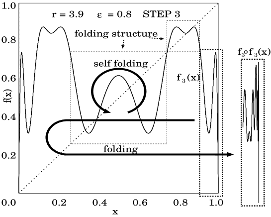
Figure 6: The folding structure. A self-contained section (SCS) folds the region outside it and itself. This is plotted at step 3, for $r=3.9$, $\epsilon=0.8$. The dynamics of the region outside the SCS are driven by the structure in the SCS.

On the other hand, the points outside of the SCS are eventually mapped to values $f_{n}\circ f_{n}(x)$ in some SCS, where they remain for all subsequent times. Following hump(s) in an SCS, the function in the remaining part can also be folded, as shown in Fig.6. The hump in the SCS can lead to a successive folding structure within itself and also in the remaining part, whose $f(x)$ is mapped to the SCS. This SCS plays an important role in classifying the types of functions.

The limiting function $\lim_{n\rightarrow\infty}f_{n}(x)$ is plotted as a function of $r$ and $\epsilon$ in Fig.10. Here, one dot in the figure represents a value of $f_{n}(x)$ in a flat piece or on a peak of the map. This figure looks similar to the bifurcation diagram of the logistic map. In fact, this graph is identical to the bifurcation diagram of the logistic map for the case$\epsilon=1$. Although the ‘bifurcation diagram’ is distorted because of the average by the weight $\epsilon$, we can detect some similarity with the original bifurcation diagram.

In the plot, one can find structures corresponding to tangent bifurcations and other bifurcations. Also, there is ’bifurcation collapse’ corresponding to crisis [19]. Here, however, there is one significant difference. In strong contrast to the case of crisis, ‘bifurcation collapse’ occurs at different parameter values, depending on each bifurcated branch of $f(x)$ (see Fig.10). Thus, there is a new regime in the ‘bifurcation diagram’ where one branch collapses and the other remains stable.

To see what happens in this new regime, we plot two functions $f_{5}(x)$ before and after a collapse of one bifurcation branch. As is seen in Fig.11(a), when bifurcated branches coexist, there are two closed SCS. Here each SCS corresponds to a bifurcated branch. Any two branches evolve independently, because points in an SCS, plotted by the dotted squares in the figure, remain within the same SCS. Regions outside the two SCS are eventually mapped to these SCS. The folding structure in each SCS is folded by itself while the folding structures outside these SCS are folded by these SCS.

As $r$ or $\epsilon$ is increased, the bifurcation collapses. As shown in Fig 11(b), one of the the SCS ( around $.3<x<.7$) collapses while the other remains. Some parts of the function $f(x)$ at the collapsed SCS are mapped to the SCS around $x\approx 0.8$. This is displayed in (b), where the function in the lower section ‘invades’ the upper area. This parameter region is nothing but the region where only one bifurcated branch is collapsed.

With further increase of $r$ or $\epsilon$, the SCS around $x\approx 0.8$ also collapses and they form a single SCS. This parameter regime corresponds to the region in which both the two branches are collapsed.

The change of the four phases can be understood in terms of the folding and SCS as follows.

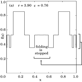
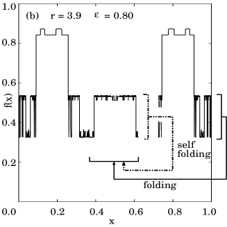
Figure 7: The folding mechanism in the SCS and the remaining part. (a) Folding process at the center region stops to form steps, but it leads to fine step structures at the edges of the map (near $x$ = 0.0 and 1.0) during the transient time, before the function (at the center) converges to a fixed function with few steps. Here, $r=3.9,\epsilon=0.76$. (b) The center structure folds itself and the part outside the SCS. This folding structure does not converge as $n\rightarrow\infty$ and forms finer and finer steps with time, leading to fractal steps. Here, $r=3.9,\epsilon=0.80$.

• (S) & (FS): As is seen in Fig.7 (a), the folding structure in an SCS continues to fold the rest of the map until it converges as $n\rightarrow\infty$. If the folding structure converges to a step function, the number of type-I fixed points no longer increases for large $n$.

  • (S): In the step phase, the folding structure in the each SCS converges to flat pieces. The points outside the SCS are not folded by the SCS.

    This phase is seen in the parameter region between the tangent bifurcation and the second bifurcation.

  • (FS): In folded step phase, the folding mechanism stops at an SCS. Until the folding structure converges, a few points, mapped to an SCS, continue to form foldings, due to step structures in the SCS. For most intervals of $x$, $f_{n}(x)$ is a step function, as in the region(S), while a few intervals exhibit fine folded structure (with a finite number of folds).

    This phase is observed in the parameter region between the second bifurcation and the first bifurcation collapse.

• (F) & (R): The folding structure in an SCS folds itself when $r$ or $\epsilon$ is large. Here, as $n$ increases, the function $f_{n}(x)$ intersects the identity function an increasing number of times. Thus, the number of type-I fixed points increases with iteration in the SCS.

  • (F): In some regions of the remaining part, the folding does not continue. Here flat pieces are formed. This process leads to a fractal phase.

    This phase exists in the parameter region between the first and the last bifurcation collapses.

  • (F)$\rightarrow$(R): With the increase of $r$, the number of bifurcation branches, as well as the number of collapsed bifurcations, increases. Infinite folding structure starts to cover the entire domain.

  • (R): In the random phase, all bifurcation branches are collapsed, and no SCS smaller than the total interval exists anymore. The entire domain forms a single SCS with self-folding structure. Hence no flat pieces remain anymore.

    This phase corresponds to the region from the last bifurcation collapse.

8 Characterization of Phases

In the present section we quantitatively characterize the four phases, considering the folding effects discussed in Sec.7. As statistical characteristics, we compute the number of discontinuous points $D$ and the Euclidean length $L$ of the fixed point function to which $f_{n}(x)$ converges after transient time steps. We then study the length of the transient time $T$ before the function converges to an attractor. Discontinuous points are the edges of the flat pieces of the map, i.e., the points where $f_{\infty}(x+1/M)\neq f_{\infty}(x/M)$, while the length is given by $\sum_{j}\sqrt{(1/M)^{2}+(f_{\infty}(x_{j}+1/M)-f_{\infty}(x_{j}))^{2}}$.

For each simulation, we choose the mesh number $M$, the function is iterated until it converges, and the numbers $D$ and $L$ are determined. The dependence on $M$ is studied as the number of mesh points is doubled.

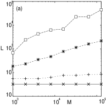
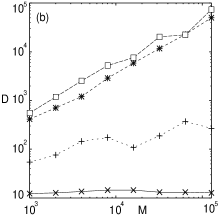
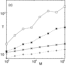
Figure 8: Log-log plot of the mesh number $(M)$ dependence of the $(L)$, $(D)$ and $(T)$: (a) the length of the graph $(L)$, (b) the discontinuous points $(D)$ and (c) the transient length $(T)$. The largest mesh size is $128000$. The length and discontinuous points are defined in the text, while the transient is measured as the time steps before an initial function is attracted to a fixed point for a given mesh. four examples from the four phases are given, with $r=3.90,\epsilon=0.60$ ($\times$); $r=3.90,\epsilon=0.76$ ($+$); $r=3.90,\epsilon=0.80$ ($*$); and $r=3.90,\epsilon=0.96$ ($\Box$). For (c), $\epsilon=0.90$ is adopted for the plot with ($\Box$) instead of 0.96.

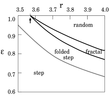
Figure 9: Phase diagram of our functional map with the initial logistic map $rx(1-x)$. The phases (S), (FS), (F) and (R) are classified according to the behavior of $L$, $D$ and $T$. The point $\epsilon=1.0,r=3.57$ corresponds to the onset of chaos of the logistic map.

The log plots of these quantities are displayed as functions of the log of the number of mesh points $M$ in Fig 8. According to the behavior of these quantities and the previous discussion on the folding structure, the four phases in Sec.7 are characterized as follows (See Fig.9).

• (S): Step (Fig.5(a))

  $D=const$, $L=const$ as $M$ increases.

  Since the folding structure does not fold the part outside the SCS, $D$ and $L$ do not change as the number of mesh points increases.

• (FS): Folded step (Fig.5(b))

  $D\propto M^{\alpha}$, $L\propto M^{\alpha^{\prime}}$, ($\alpha$, $\alpha^{\prime}<1$) for $M<M_{max}$, while they approach constants for larger $M$.

  The function $f_{n}(x)$ undergoes a stretching and folding process under the iteration, until the folding structure converges. This folding process leads to a successively finer structure, and brings about more discontinuous points with the increase of mesh points. The existence of $M_{max}$ such that for $M>M_{max}$, $D=const$ and $L=const$, is expected, because the folding structure converges. The folded region existing outside the SCS intervals is localized in a narrow interval of $x$, and the number of mesh points ($M_{max}$) necessary to observe the convergence is huge. Thus in Fig.8(a)(b), $D$ and $L$ increase with the number of mesh points, but we believe that the increase stops with a further increase of mesh points. In this region, only a finite number of such folding structures exists, and these regions are separated from other fixed points with a step function.

• (F): Fractal (Fig.5(c))

  $D\propto M^{1}$, $L\propto M^{\beta}$, ($\beta<1$).

  The function has flat pieces and folded areas, where the folding structure folds itself in each SCS. The number of type-I fixed points (thus possible values of $f_{n}(x)$) increases with iteration. Because of the folding of folding structure itself, there are some discontinuous points in any neighborhood of a point $x$ in an SCS with the bifurcation collapse. Thus, $D\propto M^{1}$ follows.

• (R): Random (Fig.5(d))

  $D\propto M^{1}$, $L\propto M^{1}$.

  Flat pieces in the function vanish, and they are replaced by folded regions. In this area there are discontinuous points around any infinitesimal neighborhood of $x$. Now, the statistical behavior of $D$ and $L$ is identical to that of a function with random values at each mesh point.

Of course, the number of type-I fixed points (possible values of $f(x)$) is a basic quantities. This number does not increase with the mesh number $M$ for (S) and (FS) phases, while it increases with $M$ for (F) and (R) phases. Roughly speaking, the increase is proportional to $M$, although there is a large variation around this, possibly due to some number theoretic complication.

In addition to the characteristics of limiting functions $\lim_{n\rightarrow\infty}f_{n}(x)$, we also study the transient process. In Fig.8(c), the length of the transient $(T)$ before the function reaches a fixed point is plotted. The transient length stays very small in (S) and (FS) phases. On the other hand, the length increases in proportion to $M^{\delta}$, in (F) and (R) phases. The exponent $\delta$ increases with $r$ in the (F) phase, and it is approximately 1/2 in the (R) phase.

This divergence of the transient length implies that the function does not converge to a fixed point function in the limit of infinite precision. The process in which a finer folding structure is formed continues forever. Note, however, that our numerical results with a finite mesh can capture the behavior of the function. Even though the function does not converge in the infinite precision limit, the dynamical change at a fine scale does not affect the larger structure. As time increases, the change in the value of $f_{n}(x)$ becomes smaller and smaller. Hence, the classification of $f_{n}(x)$ obtained with a finite-mesh simulation is valid.

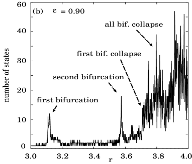
Figure 12: The parameter $r$ dependence of some characteristics. (a) The quantity $\int dxf(x)$ versus $r$ with fixed $\epsilon$. (b) The number of type-I fixed points versus $r$ with fixed $\epsilon$, with mesh size 4096. As mentioned, there are effects introduced by the finite size of the mesh: addition of pseudo type-I fixed points near a tangent bifurcation, and missing type-I fixed points with a large slope in the random phase. To remove the former effect, we count a series of 3 type-I fixed points ($x=(i-1)/M$, $i/M$, and $(i+1)/M$) as one fixed point.

Note that the phase diagram (in Fig.9) plotted with the above characteristics agrees with that obtained earlier using the bifurcation collapse and folding characteristics (see Table 1 for a summary). The phase transition is also characterized by other ‘order parameters’. In Fig.12, the quantity $\int dxf_{\infty}(x)$ and the number of type-I fixed points (the number of possible states) are plotted. From these figures, we can see the bifurcation of the phases as the parameter value is changed.

The value $\int dxf_{\infty}(x)$ is governed by a dominant step structure for small $r$. At the first and second bifurcation points, there are cusps in the integral. After the first bifurcation collapse, the integral does not change smoothly as a function of the parameter $r$. Rather, it begins to exhibit sensitive dependence on $r$. At the last bifurcation leading to the (R) phase, there is a large jump in the integral, due to the collapse of the SCS.

Such bifurcation structure is also seen in the change of the number of type-I fixed points, plotted in Fig.12(b) (for $M=4096$). The number remains small (3 or fewer) up to the second bifurcation. At the second bifurcation leading to (FS), it starts to increase slightly. After the first bifurcation collapse, the number jumps to a much larger value.

In the present and last two sections we have discussed the function dynamics for the case $\epsilon\neq 1$, starting from a single-humped map. For $\epsilon=1$, our dynamics is nothing but normal iteration of the logistic map. In this case, ‘bifurcation collapses’ occur at the same parameter. The function $f_{n}(x)$ exhibits fixed, periodic and chaotic behavior, as in the bifurcation of the logistic map. (In a finite-mesh computation, the number of type-I fixed points is much larger than the case $\epsilon<1$, while periodic points are also frequently observed there.)

9 Periodic Attractor

To this point, we have focused on the fixed point solutions in the case $\epsilon\neq 1$. Although they are not so common, periodic points of $f_{n}(x)$ are also observed in the case $f_{0}(x)=rx(1-x)$. In fact, it is often the case that a function with multiple humps evolves into a function possessing periodic points. Even in such case, the function $f(x)$ is a fixed point for most points, and only at a few points $x^{\prime}$ $f_{n}(x^{\prime})$ changes periodically. Here we study how such periodic points are constructed in the case that they depend on a finite number of type-II fixed points.

The mechanism allowing for a periodic cycle for $\epsilon\neq 1$ is different from that for the case with $\epsilon=1$, discussed in Sec.4. Here, we focus on the case $\epsilon\neq 1$. Periodic attractors for a particular $x^{\prime}$ with an arbitrary period are constructed as follows. We note that as far as we have examined extensively, a periodic point moves successively on type-II fixed points.

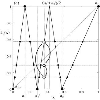
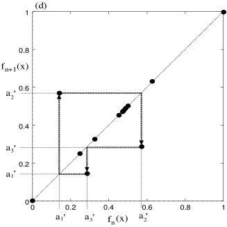
Figure 13: Periodic structures. (a) and (b) are schematic representations how at a given point $x=x^{\prime}$ (a) or $x=x^{\prime\prime}$ (b) shows a period-2 motion. In the representation, $a_{i}$ is a type-I fixed point, while $a_{i}^{\prime}$ is a type-II fixed point mapped to it. The value of $f_{n}(x^{\prime})$ changes with period 2, where $x^{\prime}$ is mapped to $a_{i}^{\prime}$. In (b), the hierarchical configuration of periodic structure is shown, where $f_{n}(x^{\prime\prime})$ changes with period 2, mapping to the periodic points $x_{i}^{\prime}$. (c) An example of $f_{0}(x)$ giving a period-3 cycle. By starting from a function given by solid line, $a_{1}=1$ and $a_{2},a_{3}=0$ are type-I fixed points, and $a_{1}^{\prime},a_{2}^{\prime},a_{3}^{\prime}$ are type-II fixed points mapped to $a_{1},a_{2},a_{3}$ respectively. Then, the function values $f_{n}(x)$ in our model at small black points are mapped with period 3 as $a_{1}^{\prime}$, $a_{2}^{\prime}$ and $a_{3}^{\prime}$, successively. As an example, the period 3 behavior is indicated by the white points and the arrows. (d) A return map with starting $f_{0}(x)$ as (c) for all ($f_{n}(x^{\prime}),f_{n+1}(x^{\prime})$) ($n=1000-1010$) with $M=8000$. All $f_{n}(x^{\prime})$ fall to a fixed point or a period-3 attractor. In general, a map with $k$ humps has the possibility to form $k$-periodic points.

For example, let us design a period-2 solution with $f_{2n}(x^{\prime})$ ($f_{even}(x^{\prime})$), $f_{2n+1}(x^{\prime})$ ($f_{odd}(x^{\prime})$) and $f_{m+2}(x^{\prime})=f_{m}(x^{\prime})$. Our purpose is to arrange the fixed points so that $f_{n}(x^{\prime})$ is mapped to two different fixed points by each step. If $f_{n}(x^{\prime})$ is mapped to a type-I fixed point, $f_{n}(x^{\prime})$ becomes a type-II fixed point. Here, we treat such a case that $x^{\prime}$ is mapped to a type-II fixed point. In this case, to have period-2 solution of $f_{n}(x^{\prime})$, 2 type-I fixed points and 2 type-II fixed points must be chosen. We denote type-I fixed points as $a_{1}$ ($f(a_{1})=a_{1}$) and $a_{2}$ ($f(a_{2})=a_{2}$) and the correspondent type-II fixed points as $a_{1}^{\prime}$ ($f(a_{1}^{\prime})=a_{1}$) and $a_{2}^{\prime}$ ($f(a_{2}^{\prime})=a_{2}$). Now we consider the situation shown in Fig.13(a), where it is assumed $f_{even}(x^{\prime})=a_{1}^{\prime}$ and $f_{odd}(x^{\prime})=a_{2}^{\prime}$. The condition for period-2 is given by

$$\left\{\begin{array}[]{lclcl}f_{odd}(x^{\prime})&=&(1-\epsilon)f_{even}(x^{\prime})&+&\epsilon f\circ f_{even}(x^{\prime})\\ f_{even}(x^{\prime})&=&(1-\epsilon)f_{odd}(x^{\prime})&+&\epsilon f\circ f_{odd}(x^{\prime})\end{array}\right.$$ (7)

which is written as

$$\left\{\begin{array}[]{r}a_{2}^{\prime}=(1-\epsilon)a_{1}^{\prime}+\epsilon a_{1}\\ a_{1}^{\prime}=(1-\epsilon)a_{2}^{\prime}+\epsilon a_{2}\end{array}\right.$$ (8)

From this equation, $a_{1},a_{2}$ are determined by $a_{1}^{\prime},a_{2}^{\prime}$ (or vice versa) as

$$\left(\begin{array}[]{c}a_{1}^{\prime}\\ a_{2}^{\prime}\end{array}\right)=\frac{\epsilon}{1-(1-\epsilon)^{2}}\left(\begin{array}[]{cc}(1-\epsilon)&1\\ 1&(1-\epsilon)\end{array}\right)\left(\begin{array}[]{c}a_{1}\\ a_{2}\end{array}\right)$$ (9)

If this condition is satisfied for $a_{1}$,$a_{2}$,$a_{1}^{\prime}$ and $a_{2}^{\prime}$, $f_{n}(x^{\prime})=f_{n+2}(x^{\prime})$.

A function of an arbitrary period is constructed in the same way as one of period 2. To construct a solution of period $N$, we introduce $N$ type-I fixed points denoted by $a_{i}$ $(i=1,2,\ldots,N)$ and $N$ corresponding type-II fixed points denoted by $a_{i}^{\prime}(i=1,2,\ldots,N)$ with $f_{n}(a_{i}^{\prime})=a_{i}(i=1,2,\ldots,N)$. For $f_{n}(x^{\prime})$ to change the values $a_{i}^{\prime}$ $(i=1,2,\cdots,N)$ cyclically, the fixed points have to satisfy the condition

$$\left(\begin{array}[]{c}a_{1}^{\prime}\\ a_{2}^{\prime}\\ \vdots\\ a_{N}^{\prime}\end{array}\right)=\frac{\epsilon}{1-(1-\epsilon)^{N}}\left(\begin{array}[]{ccccc}(1-\epsilon)^{N-1}&(1-\epsilon)^{N-2}&(1-\epsilon)^{N-3}&\ldots&1\\ 1&(1-\epsilon)^{N-1}&(1-\epsilon)^{N-2}&\ldots&(1-\epsilon)\\ \vdots&\vdots&\vdots&\ddots&\vdots\\ (1-\epsilon)^{N-2}&(1-\epsilon)^{N-3}&(1-\epsilon)^{N-4}&\ldots&(1-\epsilon)^{N-1}\end{array}\right)\left(\begin{array}[]{c}a_{1}\\ a_{2}\\ \vdots\\ a_{N}\\ \end{array}\right)$$ (10)

.
which is obtained in the same way as in the period-2 case.

If an initial function is continuous and has the type-I and II fixed points $a_{i}$ and $a_{i}^{\prime}$ for $i=1,\ldots,N$, there are some points $f_{n}(x^{\prime})$ which are period $N$. An example of the shape of such a $f_{0}(x)$ is displayed in Fig.13(c) for the case $N=3$. The map has period-3 points plotted with small black points. If all $a_{j}$ except one are $0$, the function of period $N$ has $N$ hills and $N$ valleys. Indeed, an $N$-humped initial function has the potential to possess period-$N$ points.

We have carried out simulations starting from an initial function with many humps. As expected, the limiting function consists of type-I and type-II fixed points, that form a step, folded step, fractal, and random phases, depending on $\epsilon$ and the height of the humps. Within these structures, periodic points are embedded. For several values of $x^{\prime}$, the function $f_{n}(x^{\prime})$ falls on the same periodic cycle mapping the same type-II fixed points. In Fig.13(d), the return map starting from Fig.13(c) for all $(f_{n}(x^{\prime}),f_{n+1}(x^{\prime}))$ is displayed ($n=1000-1010$). This return map was produced given by a computer simulation with $M=8000$. All $f_{n}(x^{\prime})$ fall onto a fixed point or onto a period-3 attractor, and $f_{n}(x)$ is a period-3 function as a whole.

The values of the period-3 function $f_{n}(x^{\prime})$ for several points $x^{\prime}$ often oscillate synchronously with the same phase. Before $f_{n}(x)$ falls onto a periodic point, the function often takes the same $f_{n}(x)$ value for several values of $x$. Later, the function $f_{n}(x)$ is mapped to type-II fixed points, and starts to form a cycle. In this case, all $f_{n}(x)$ for these $x^{\prime}$ values oscillate synchronously.

Hierarchical organization of periodic points is also possible. Noting that for a $k$-periodic point $f_{n}(x^{\prime})$ takes the same value every $k$ steps, we can construct a new periodic point by utilizing other periodic points. First, we select one period-$k$ point. If another point $f_{n}(x^{\prime\prime})$ is mapped to this point after $k$ steps, the $k$-periodic $f_{n}(x^{\prime})$ acts as a fixed point for $f_{n}(x^{\prime\prime})$, and a consistent hierarchical equation can be constructed. For this, we have to prepare period-$k$ points $x_{1}^{\prime},\cdots,x^{\prime}_{k}$ that are used to make a new period-$k$ point, where each $k$-periodic point acts as a fixed point for $x^{\prime\prime}$ per $k$ steps. Thus, the required number of $k$-periodic points to make a new one is $k$. If each period-$k$ point acts as a fixed point for $f_{n}(x^{\prime\prime})$, $f_{n}(x^{\prime\prime})$ will also have period $k$. Thus, we can obtain a hierarchical periodic point $f_{n}(x^{\prime\prime})$ depending on other periodic points.

For example, we select two period-2 points (see schematic configuration Fig.13(b)). Two period-2 points, $f_{n}(x_{1}^{\prime})$ and $f_{n}(x_{2}^{\prime})$ are mapped to type-II fixed points as $f_{even}(x_{1}^{\prime})=a_{11}^{\prime}$, $f_{odd}(x_{1}^{\prime})=a_{12}^{\prime}$, and $f_{even}(x_{2}^{\prime})=a_{21}^{\prime}$, $f_{odd}(x_{2}^{\prime})=a_{22}^{\prime}$, respectively. If $f_{n}(x^{\prime\prime})=x_{1}^{\prime}$ for even $n$ and $f_{n}(x^{\prime\prime})=x_{2}^{\prime}$ for odd $n$, $f_{n}(x^{\prime\prime})$ is mapped $a_{11}$ and $a_{22}$ alternatively. This condition is given by

$$\left\{\begin{array}[]{lcl}f_{odd}(x^{\prime\prime})&=&(1-\epsilon)f_{even}(x^{\prime\prime})+\epsilon a_{11}^{\prime}\\ f_{even}(x^{\prime\prime})&=&(1-\epsilon)f_{odd}(x^{\prime\prime})+\epsilon a_{22}^{\prime}\end{array}\right.$$ (11)

The above equation has the same form as equation (9). If $a_{11},\ldots,a_{22}$ and $a_{11}^{\prime},\ldots,a_{22}^{\prime}$ support two period-2 points and $x_{1}^{\prime},x_{2}^{\prime},a_{11}^{\prime}$ and $a_{22}^{\prime}$ satisfy the above condition, $f_{n}(x^{\prime\prime})$ evolves by period-2.

In the same way period-$k$ points which depend on $k$ period-$k$ points can be constructed. Also, hierarchical construction for the next level periodic function can be carried out in the same manner.

In the fractal and random phases, the evolution leads to infinite type-I fixed points. In the present paper, however, we have discussed only the construction of periodic solutions using a finite number of type-I and type-II fixed points. If there is a continuous interval consisting entirely of type-II or type-I fixed points, the evolution of the function itself starts to be governed by some mapping generated by this interval of fixed points. Then, quasi-periodic, chaotic, and ‘meta-chaotic’ evolutions of function are possible, as will be discussed in a subsequent paper [15].

10 Summary

In the present paper, we have introduced a simple functional map to consider a dynamical system in which rules and variables (or objects) are not distinguished at the initial time. A simple (possibly the simplest) universal model was introduced to study such a situation, as a map describing the dynamics of a function.

As a first step, we studied the case in which the dynamics are given simply by $f\circ f(x)$, which can be thought of as defining the way the network is reconnected. Its elementary cyclic structures were revealed. In Sec.4, we illuminated some of the basic structures of our functional map. We found that the type-I and type-II fixed points provide the elementary core structure. A type-I fixed point is mapped to itself under $f(x)$ ($x^{I}=f(x^{I})$) and forms a basis of symbolization in the abstract language space ($x$). A type-II fixed point $x^{II}$ is mapped to a type-I fixed point under $f(x)$ ($x^{I}=f(x^{II})$. The concept of a self-contained section (SCS) was also introduced as a region in which the functional dynamics remain confined within the the region in question.

The articulation process studied here is a process in which intervals of $x$ are classified according to how $f_{n}(x)$ converges to divided intervals consisting of type-II fixed points, while each type-I fixed point corresponds to a symbol for each articulated object. The function as a filter articulates the continuous world $x$ into a set of segments on each of which $f_{n}(x)$ assumes a distinct constant value.

Starting from a monotonic function, a piecewise constant solution is reached as a fixed function. Each step consists of a continuous set of type-II fixed points mapped to the same type-I fixed point. This step function is the simplest example for the articulation process. In Secs.5-8, we studied the evolution from a single humped map, where the folding of the function to itself can lead to many type-I fixed points. Depending on the degree of folding, the limiting forms of $f_{n}(x)$, $\lim_{n\rightarrow\infty f_{n}(x)}$ are classified as step (S), folded step (FD), fractal (F) and random (R) phases. These phases are characterized by the mesh number dependence of the number of type-I fixed points and discontinuous points and of the length of the function defined in Sec.8. (see Table 1).

In the step and folded step phases, as in the case for a monotonic function, our functional dynamics lead to a partition of $x$ into a continuous interval $[x_{i},x_{i+1}]$ in which $f(x)$ assumes a constant value ($const_{i}$). Rigid, fixed articulation structure is formed there. The difference in the degree of folding distinguishes the (FS) and (S) phases. In the fractal and random phases, the function successively forms smaller and smaller articulation structures (Secs.6, 7). In the fractal phase, successive foldings are restricted within SCS and $f_{n}(x)$ outside the SCS is folded by the SCS. In the random phase, the whole interval folds itself and forms successively smaller structures. In these two phases, finer structures are formed successively, and a fixed point function is not reached in the limit of an infinite number of mesh points. In Sec.9, we constructed periodic functions using a finite number of fixed points. Hierarchical periodic points were also constructed by assuming new periodic points $x^{\prime\prime}$ mapped to a higher-level periodic point $x^{\prime}$ ($f(x^{\prime\prime})=x^{\prime}$).

11 Discussion

Note that the type-I and type-II fixed points provide a basis to have the five requisites discussed in Sec.1. These fixed points give a core structure to the network, obtained through the iteration process. One might say, in some sense, that with the emergence of type-I and type-II fixed points, code and encoding become separated. Such separation is not limited to these two types of fixed points. The distinction between SCS and the points outside these provide a separation of self-referenced units and the structure mapped to them. Summing up, the evolution of our dynamics can capture

• core structure (prototypes) as fixed points

• folding structure (categories) in SCS, which leads to the articulation of the network and alters the folding structure itself

• the points outside SCS intervals that are mapped to some SCS (entailed categorization by categories)

Note that the above described structure of our model corresponds well with the separation of cognition and notion, in language. Out of an inarticulate and time-variant network, some invariant structures are separated as a rigid structure through iterations. This rigid structure, at the lowest level, is given by fixed points, while a set of SCS provides such rigid structure at a higher level. The configuration of fixed points can provide a base for periodic motion of other points, while SCS have the role of controlling the remaining, vague part. With the rigid parts, some structures are articulated. This rigid part provides a basis to describe the web of relationships or circulation of signs.

When an initial function (a single-humped map) is given, the SCS for the function is the whole domain. Through iterations, time-invariant parts and time-variant parts can be separated. The dynamics of variant part (that outside SCS intervals) is governed by that of the function within the invariant (SCS) part, while the invariant part also is mapped to variant parts before it forms the SCS. During the transient process to form the invariant part, the dynamics of the invariant part may depend on variant parts also. In addition to the above roles of the variant part, it can create some relationships between elements within it.

The function $f(x)$ for points $x$ outside the SCS intervals can form some relationships through the folding mechanism before the function is mapped into SCS. For example, synchronization $f_{n}(x^{\prime})=f_{n}(x^{\prime\prime})$ can be reached during the transient step before the function is mapped to a rigid part. Although the rigid invariant part governs the dynamics of $f_{n}(x)$ later, this synchronization relationship, which is invariant later, is determined only by the dynamics within the variant part. We may say that the invariant part is the basis to describe the circulation of signs (the rigid part being a ‘stable element’ in the sea of relations), and that the dynamics of the variant part is determined by the invariant part. After some iterations, the synchronization is dealt as ‘social’ redundancy by the invariant part.

In fact, within this context, the term ‘prototype’ was introduced in cognitive linguistics [10]. For example, language is constrained by the structure of the human body. The linguistic structure (prototype and category) suitable for the human body (which enables one to iterate language as symbols) is the foundation for the speech act. The basic structure of the human body is common for all humankind, and for this reason we have common linguistic structure. This common structure is rigid (invariant) with respect to the iteration, just like the fixed point of our model. This rigidness provides the possibility of speech act that is common in a society. Of course, if the entire articulation is common for all individuals, there is no novelty. The prototype gives only a foundation for language and the category can be articulated in various ways.

Although the speech act is restricted by the condition of the body, there is some redundancy in the language network with regard to describing something. In our system, such redundancy is seen in the points lying outside the SCS intervals, where some ‘synchronization’ is generally observed, driven identically by a prototype structure in SCS. Such ‘synchronization’ is attained through iteration of the functional mapping within the region outside the SCS intervals, before $f(x)$ is mapped to $x$ in an SCS.

With the change of the bifurcation parameter in our model, a section is no longer an SCS when a function value in the section starts to be mapped to outside of the section. Then, a larger network structure with mutual reference is formed, as is seen in the collapse of bifurcation in our model. Such collapse of prototype structure is also a concern of cognitive linguistics.

In the fractal and random phases of our model, successively smaller core structures are formed through the folding process. Novel core structures can be formed ceaselessly in principle. In these phases, the network exhibits a variety of articulation structures, which have sensitive dependence on the initial network. This diversity in the network is a consequence of our model, where, in contrast to typical artificial intelligence studies, rules and objects are not separated in the beginning, and a table between the two is not given in advance.

It should be noted that the above described structure of prototype and category, as well as the capacity for novelty and diversity, are a consequence of a dynamical system with a self-reference term and initial folding structure. Such structure is universally observed as long as our dynamics includes $f\circ f$ and some folding structure, given for example, by a humped mapping. In this sense, we may hope that the present study gives a first step to understand dynamic separation of prototype and category in language, although the model may be abstract and metaphorical at the present stage.

As mentioned in Sec.1, such separation is not limited to language, but is often seen in biology, for example, in the separation of function between DNA and protein. Since self-replication processes in life require a self-referential structure., the present study may give some insight into biological organization [26]

With folding structure, a function does not always reach a fixed point for all $x$ values. In Sec.9, we explicitly demonstrated the existence of periodic motion of a function value by choosing an initial function suitably. The value is mapped to several type-II fixed points periodically. The connection defined by $x\rightarrow f(x)$ dynamically moves over articulated type-II fixed points that are mapped to a ‘core symbol’ (type-I fixed point). Hence, a dynamic syntax is formed in a hierarchy of periodic points. In Sec.9, periodic points mapped to such periodic points are also constructed. Thus, rules over rules can be formed in our model. As mentioned in Sec.1, organization of a meta-rule is important in biological problems, including development, cognition, and language. In a subsequent paper we will report on how a rule of a one-dimensional map is formed within our functional dynamics, which allows for periodic, quasi-periodic, chaotic dynamics. There it will be shown explicitly that a rule to change a one-dimensional map itself can be embedded in our functional equation, which allows for ‘meta-chaotic’ dynamics, where the rule itself changes chaotically, and the orbital instability is stronger than exponential in time. With these dynamical structures, modalities of rule, meta-rule, meta-meta rule, $\cdots$ will be formed successively.

In this article, we have studied the case with only one function $f_{n}(x)$. In other words, there is only one self-feedback process for one agent. This use of a single function is, of course, not sufficient to discuss ‘social’ aspects of language. For this, functional dynamics with multiple functions $f^{i}_{n}(x)$ (with the term $f^{i}_{n}\circ f^{j}_{n}(x)$) should be considered, to see the articulation and rule-generation process in a society of agents [23]. Note that the results in the present paper are for a special case when the functions agree ($f^{i}_{n}(x)=f^{j}_{n}(x)$) through iterations. Indeed, we have often observed such agreement in some preliminary simulations of the multiple functional dynamics case, where the present argument is valid.

Of course, some other extensions should be considered in the future, including the use of a space of higher-dimension than the one-dimensional space used here, ‘sequential dynamics’ instead of ‘parallel dynamics’ applied to $x$, the addition of noise to smooth $f(x)$, and so forth. Indeed, some preliminary studies suggest that the basic structures presented in this paper are valid for these extensions.

Finally, it should be mentioned that self-reference structure is mathematically studied as domain theory [24][25][26], where consistent and non-trivial sets including $f\circ f$ are constructed. Although there may be some relationship between our fixed-point functions and domain theory (and the establishment of such a relationship will be an important future study), the dynamics in the present approach are missing in domain theory. A bridge between dynamical systems theory and domain theory may be required to construct a mathematical foundation of our functional dynamics, in addition to the construction of a suitable functional space to support our function.

Appendix A Appendix

In this appendix we investigate the equation (4) with a ‘discrete mesh’ (see Sec.4). A simple network which consists of elements arranged cyclically was introduced in Sec.4. In general, an initial network is given as $f_{0}(i)=j(i,j=0,\ldots,M-1)$. In this equation, the functional map changes only the connection from the element $f(i)$ to the element to which the mapped element $f(i)$ is mapped, that is $f_{n}\circ f_{n}(i)$. Here we study the dynamics of such a connection changing among a finite number of elements.

A fixed point is classified as either type-I or II, as mentioned in Sec.3. The value $f(i)$ for these fixed points remains unchanged through the iteration.

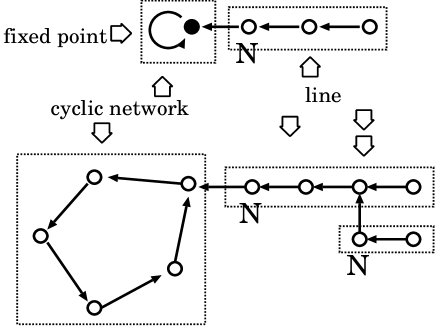
Figure 14: Classification of the network. Once an initial network is given, it is separated into cyclic networks and lines.

When an initial function (i.e., the connection in the graph) is given, the graph is separated into two parts (See Fig.14):

(i) a cyclic network which consists of $M$-elements (If $M=1$, it is type-I fixed point.)

(ii) a line defined as an $N$-length line which does not belong to (i) but connects to either (i) or another (ii) line.

The initial network is represented by a combination of these restricted graphs that are drawn in one stroke, since the number of elements is finite and each element $i$ has one value $f(i)$. The allowed graphs are only cyclic networks and lines. A cyclic network is a set of elements in which a bijection exists. In other words, $f_{0}(i)$ ($i=1,2,\ldots,M$) takes a different value for each $i$ in the set, and there is one element $i$ in the set for each $j$ that satisfies ${f_{0}}^{n}(i)=j$ ($n=1,2,\ldots,M$). Hence, the elements of the set are arranged in a cyclic manner. Each element $i$ that belongs to this network satisfies ${f_{0}}^{M}(i)=i$, where $f^{n}(x)$ is the $n$th iterate of the function $f$. A line consists of $N$ elements, while each element $i$ is mapped to $f_{0}(i)=i+1$ for $i=1,2,\ldots,N$ as displayed in Fig.14. The last element $N$ is, by $f_{0}(N)$, mapped to another line or a cyclic network.

If a given initial network possesses some lines, as is easily understood, the network has at least one line that is mapped to a cyclic network (including a type-I fixed point). With the time evolution, lines are attracted to the structure to which element $N$ mapped. Finally, each element which belongs to this line is mapped to an element that belongs to a cyclic network (i.e., $f^{n}(i)$ belongs to a cyclic network). At this stage, elements on the same line evolve in the same way as the elements in the limiting form of the cyclic network.

Hence, to discuss the behavior of the limiting form of the network (i.e., $f^{n}(i)$ with large $n$), we need to consider only the evolution of the $M$-element cyclic network. Under the iteration of the function, the network is either reduced to disintegrated parts or remains a cyclic network. We call the network ‘elementary’ if it is not disintegrated into parts under the iteration of the function. A one-element cyclic network (i.e., type-I fixed point) is obviously ‘elementary’.

We can always arrange the $M$ elements on a circle, in a cyclic manner as $i$, $f(i)$, $f\circ f(i)$, $f\circ f\circ f(i)$$\cdots$. Here we call this $f_{0}(i)$ a ‘cyclic network’. The evolution of a cyclic network of $m$ elements is shown in Fig.1 for $M=1,2,\ldots,7$.

We can compute the period ($P(M)$) for each cyclic network. In this case, each element $i$ connects to its left-hand neighbor at first. After the first iteration, the connection is changed to the next nearest neighbor $i+2$. With the next iteration, the connection is changed to $i+4$. In this way, after $n$ iterations, the connection has changed to $i+2^{n}$. Since the element is mapped to $2^{n}\pmod{m}$ neighbor at the $n$th step, it is convenient to introduce the $a_{n}$ given by

$$a_{n+1}=2a_{n}\pmod{M}$$ (12)

with $a_{0}=1$.

When $a_{n}$ reaches $a_{n}=1$, the $M$ elements form a cycle of period $n$. On the other hand, if $a_{n}$ coincides with one of previous $a_{i}$ $(i=1,2,\ldots,n-1)$, the network is reduced to a cycle with a period that is a divisor of $M$.

As seen in Sec.4, a cyclic network consisting of an even number of elements is reduced to disintegrated elementary networks, while a cyclic network consisting of an odd number elements is elementary. By simple calculation, periods of some particular series can be obtained, such as $P(2^{n}-1)=n$ and $P(2^{n}+1)=2n$. It is also found that there is a function $\Phi(M)$ such that $P(M)\leq\Phi(M)$ from Euler’s theorem. Here, the function $\Phi(M)$ ($M$ is odd) is defined as follows. Let us first decompose $M$ into factors of prime numbers as $\prod_{k=1}^{m}{p_{i}}^{\alpha(i)}$, where $p_{i}$ as a prime number. Then $\Phi(M)$ is defined as the least common multiple among the values ${p_{i}}^{\alpha(i)-1}(p_{i}-1)$ for $i=1,2,\ldots,m$. $\Phi(M)$ satisfies $2^{\Phi(M)}\equiv 1\pmod{M}$, but it is not necessarily the smallest integer satisfying the condition. Hence, the above inequality $P(M)\leq\Phi(M)$ is obtained.

Now let us consider the evolution of a network from a general initial condition. If there are cyclic networks in the initial graph, the elements in the cyclic networks fall onto an elementary network, and they remain in this elementary network. The cyclic network evolves only within the elements included in the initial network (i.e., $f^{k}(x)$ belongs to the network), while the elements belonging to a line are eventually attracted to the network that the last element of the line is mapped to.

Now it is clear how the initial $f_{0}(i)$ is reduced to a combination of elementary networks. With the initial function, its configuration has been classified into (i) and (ii). The final function $f_{n}(i)$ with $n\rightarrow\infty$ is given by elementary networks (including type-I fixed points), and the elements that are connected to them. If the elementary network is a type-I fixed point, elements on the line connected to it form type-II fixed points.

Acknowledgments

The authors would like to thank Drs. T. Ikegami and S. Sasa for discussions. This work is partially supported by Grant-in-Aids for Scientific Research from the Ministry of Education, Science and Culture of Japan. One of authors (NK) is supported by a research fellowship from the Japan Society for the Promotion of Science.

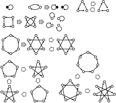
Figure 1: Time evolution of cyclic networks with $M=1,2,\ldots,7$. The network with $M=3$ has period 2, that with $M=5$ has period 4, and that with $M=7$ has period 3. The network with $M=4$ is reduced to 4 disintegrated fixed points and that with $M=6$ is reduced to two disintegrated $M=3$ networks. The algorithm to decide the period (see the Appendix) for $M=3$ is given by $a_{0}=1,a_{1}=2,a_{2}=1$, and the period is thus 2. For $M=5$, the algorithm proceeds as $a_{0}=1,a_{1}=2,a_{2}=4,a_{3}=3,a_{4}=1$, and the period is 4.

Figure 2: The period $P(M)$ plotted for elementary networks for odd $n$.

Figure 3: Time evolution of $f_{n}(x)$ ($n=0,1,2.$) for $r=3.90,\epsilon=0.80$. The number of type-I and type-II fixed points increases with time. Circles indicate fixed points, while arrows indicate type-I fixed points, at which $f_{n}(x)$ intersects the identity function. With the $\epsilon f_{n}(x)\circ f_{n}(x)$ term, the function is distorted from the simple iteration of the logistic map.

Figure 4: For an initial continuous monotonically increasing function $f_{0}(x)$, the corresponding $f_{\infty}(x)$ after the evolution is plotted (here $f_{100}(x)$ is plotted with $f_{0}(x)$). Once the initial function is given, the intervals in which $f_{0}(x)>x$ or $f_{0}(x)<x$ are determined as encircled by the dotted line. In each interval, $f_{\infty}(x)$ takes the same value as type-II fixed points.

Figure 5: Four typical results of numerical simulations of our functional map, with $M=4096$, plotted at step 100, when $f(x)$ has converged to a fixed function. (a) $r=3.9,\epsilon=0.60$, (b) $r=3.9,\epsilon=0.76$, (c) $r=3.9,\epsilon=0.80$, (d) $r=3.9,\epsilon=0.96$. By increasing $r$ or $\epsilon$, discontinuous jumps spread all over the domain.

Figure 10: Bifurcation diagram. Values of limiting forms of $f(x^{\prime})$ for all $x^{\prime}$ (i.e., the values of all fixed points of $f_{\infty}(x)$) are plotted versus $r$ with fixed $\epsilon$ for all $x^{\prime}$. The values $f(x^{\prime})$ for all $x^{\prime}$ are overlaid after the function converges under the iteration of the functional map. (Thus, each point gives a value of a fixed point.) (a) $\epsilon=0.7$, (b) $\epsilon=0.8$, (c) $\epsilon=0.9$. Bifurcation collapse occurs at the parameter value where the points start to scatter. This gives the onset of phase (F).

Figure 11: The function $f_{5}(x)$ is plotted for (a) $r=3.80,\epsilon=0.90$ and (b)$r=3.83,\epsilon=0.90$. They correspond to parameter values before and after the collapse of the lower bifurcation branch. In (a), there remain 2 self-contained sections indicated by the squares. In (b) the SCS at the lower value is collapsed, while the upper SCS remains.

Figure 15: Table 1: Characteristics of the four phases.

References

- [1] F. Waismann, ”Ludwig Wittgenstein and The Vienna Circle” Oxford U.P., 1979
- [2] A. J. Ayer, ”Language, Truth and Logic” Revised Edition. Victor Gollancz, Ltd. London, 1946
- [3] N. R. Hanson, ”Patterns of Discovery” Cambridge U. P., 1958
- [4] W. V. Quine, ”From a Logical Point of View” Harper & Row, 1963
- [5] J. L. Austin, ”How to Do Things with Words” Oxford, 1960
- [6] J. Searle, ”Speech Acts”, Cambridge U.P., 1970
- [7] Ferdinand de Saussure, ”Cours de linguistique géneŕale” Lausanne et Paris, Payot, 1916
- [8] N. Chomsky, ”The logical Structure of Linguistic Theory” Mimeographed, MIT Library, 1955. [The logical Structure of Linguistic Theory. New York: Plenum.1975]
- [9] Gilles Deleuze, ”Le pli, Leibniz et le baroque” Ed.Minuit, 1988.
- [10] George Lakoff, ”Women, Fire, and Dangerous Things” The University of Chicago Press, 1987.
- [11] J. E. Hopcroft, J. D. Ullman ”Introduction to Automata Theory, Languages, and Computation” Wesley Pub Co, 1979.
- [12] J. L. Borges, Edit. Emecé, ”FICCIONES” Buenos Aires, 1944.
- [13] P. Grim, ”Self-Reference and Chaos in Fuzzy Logic” IEEE Trans. Fuzzy Systems, 1 (1993) 237-253
- [14] I.Tsuda, ”A logic-base dynamical theory for a genesis of biological threshold” Biosystems, 42 (1997) 45-64
- [15] N. Kataoka, K. Kaneko, ”Functional Dynamics II : Syntactic Structure” in preparation.
- [16] J. M. Deutsch, ”Noise-Induced Phases of Iterated Functions” Phys. Rev. Lett. 52 (1984) 1230.
- [17] J. M. Deutsch, ”Aggregation-disorder transition induced by Fluctuating random forces” J.Phys. A.: Math. Gen. 18 (1985) 1449-1456.
- [18] M.J. Feigenbaum, ”The universal metric properties of nonlinear transformations” J. Stat. Phys. 21 (1979) 669
- [19] C. Grebogi, E. Ott and J.A. Yorke, ”Crises, Sudden Changes in Chaotic Attractors and Chaotic Transients” Physica D 7, 181 (1983c)
- [20] M. Yamaguti and M. Hata ”Takagi function and its generalization” Japan J. Appl. Math. 1 (1984) 186-199
- [21] K. Kaneko, ”Fractalization of Torus” Prog. Theor. Phys. 71 (1984) 1112-1115;
- [22] T. Nishikawa and K. Kaneko, ”Fractalization of Torus as a Strange Nonchaotic Attractor” Physical Rev. E. 54 (1996) 6114-6124
- [23] N. Kataoka, K. Kaneko, ”Functional Dynamics III : Dialogue and Community” in preparation.
- [24] G. D. Plotkin, ”Domains” Unpublished lecture notes, Dept. Computer Science, University of Edinburgh, 1983
- [25] J. Soto-Andrade, F. J. Varela, ”Self-Reference and Fixed Points: A Discussion and an Extension of Lawvere’s Theorem” Acta Applicandae Mathmaticae 2 (1984) 1-19.
- [26] R. Rosen. ”Life Itself : A Comprehensive Inquiry into the Nature, Origin, and Fabrication of Life (Complexity in Ecological Systems Series)” Columbia U. P., 1991