A dynamical model of non regulated markets

The main focus of this work is to understand the dynamics of non regulated markets. The present model can describe the dynamics of any market where the pricing is based on supply and demand. It will be applied here, as an example, for the German stock market presented by the Deutscher Aktienindex (DAX), which is a measure for the market status. The duality of the present model consists of the superposition of the two components - the long and the short term behaviour of the market. The long term behaviour is characterised by a stable development which is following a trend for time periods of years or even decades. This long term growth (or decline) is based on on the development of fundamental market figures. The short term behaviour is described as a dynamical evaluation (trading) of the market by the participants. The trading process is described as an exchange between supply and demand. In the framework of this model there the trading is modelled by a system of nonlinear differential equations. The model also allows to explain the chaotic behaviour of the market as well as periods of growth or crashes.
PCAS numbers: 01.75.+m, 05.40.+j, 02.50.Le
Contribution to the technical seminar 22/12/98, DESY-IfH Zeuthen

The traditional approaches of pricing models (indices, stocks, currencies, gold, etc.) are related to combinations of economic figures like profit or cash-flow and their expected development. Indeed, these fundamental figures are related to the approximate price. However, it is well known that similar objects (companies, goods, …) can be priced on the same market quiet different. One can observe quick changes in the pricing, which can’t be explained by any change of the underlying basic figures [1].

The present model consists of two basic components:

• (Long term trend) Scaling of the price (index) based on the long term development of basic figures [3]

• (Short term trend) Pricing by the exchange between buyers (optimists), sellers (pessimists) and neutral market members

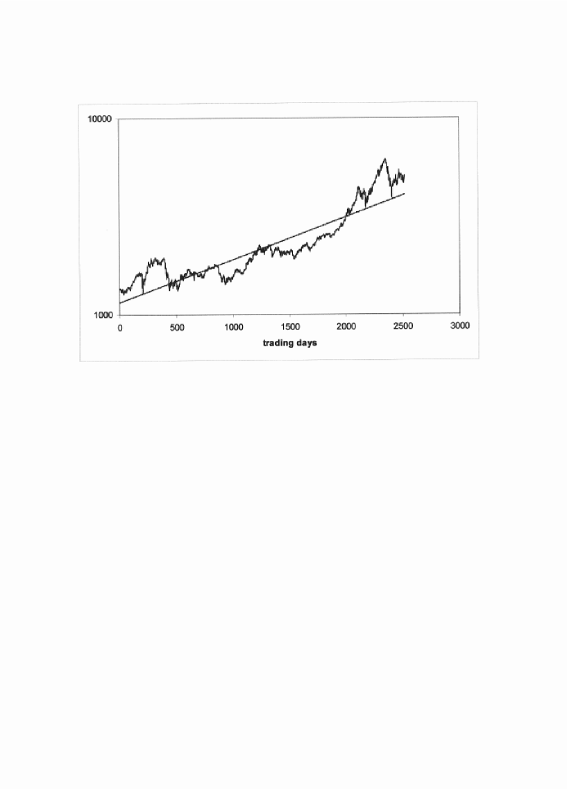
Figure 1: DAX and long term trend $I_{0}\;$ since Jan. 3. 1989

Studying, for example, the DAX $I$ for a time period of one decade one will recognise, that the basic trend $I_{0}(t)$ shows an exponential behaviour with deviations (fig. 1.). This trend can be presented as:

$$I_{0}(t)=\hat{I}_{0}\,e^{\lambda t},\;\;\mbox{with}\;\;\hat{I}_{0},\lambda=const.$$ (1)

The parameter $\hat{I}_{0}$ is the starting value: $\hat{I}_{0}(t)\equiv I_{0}(t=0)$. The growth rate $\lambda$ can variate on different markets. This parameter summarises all basic influences on the market, such as economic freedom, taxes, social-economic parameters, infrastructure and others. Comparing different markets one will find, that certain economics are growing (US, Europe) while others are declining over years (Japan ).

The value for the parameter $\hat{I}_{0}$ and $\lambda$ can be fitted from the historical market data using the least square method. The development $I_{0}(t)$ symbolises the average growth of the economy which is measured in various economic figures. The growth in (1) fulfils the Euler equation, describing the “natural” growth of unlimited systems:

$$I_{0}^{\prime}(t)-\lambda I_{0}(t)=0$$ (2)

where $y^{\prime}(t)\equiv\frac{d}{dt}y(t)$. The function (1) describes a real growth process.

As far as there is no universal pricing model, the individual evaluations by the market participants differ and the price deviates from the fundamental average. These different evaluations which are changing in time lead to some kind of spontaneous oscillations. As far as each market has another scale it is useful to normalise the market index (price) to make different markets better comparable:

$$I(t)\rightarrow i(t)=\frac{I(t)}{I_{0}(t)}$$ (3)

The function (3) performs a normalisation which will project all indices of real markets to a unitarian index $i$ with a constant basic trend: $i_{0}(t)\equiv 1$ and $\lambda=0$. This way the development of markets can be compared in a single scheme.

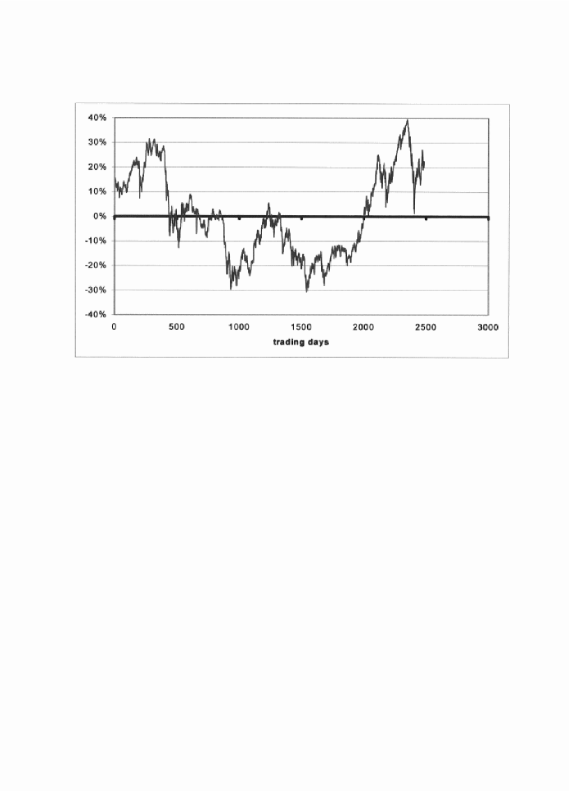
Figure 2: DAX and deviation from long term trend $\Delta i\;$ since Jan. 3. 1989

For further discussions it is necessary to define the market structure. A market is the totality of all market members participating in the trading process [2]. The total amount of market members on normalised markets (3) is constant. The normalised DAX can be found in (fig. 2.).

As already mentioned above, the subjective evaluations of the market status differ from each other [1]. The market participants can be separated into three groups: optimists, pessimists and neutral market participants. Each group has a certain concentration which evolves in time $c_{k}(t)$. Based on the normalisation there is:

$$c_{o}(t)+c_{p}(t)+c_{n}(t)=1,$$ (4)

with $c_{o}(t)$, $c_{p}(t)$ and $c_{n}(t)$ as the corresponding concentrations

The dynamics of the market is a result of the development of the $c_{k}(t)$ and the index $i(t)$. Each market group has certain features and react on market changes in a different way:

• Optimists consider the market to be priced low. They want to buy.

• Pessimists consider the market to be priced high. They want to sell.

• Neutral market members consider the market to be priced fair. They are passive.

The groups have different sizes. Comparing a typical daily trading volume with the total market capitalisation one will find that it is orders of magnitude smaller ($<1\%$). This leads to the following relation between the concentrations:

$$c_{o}(t),c_{p}(t)<<c_{n}(t).$$ (5)

Using (4) the dimension of the problem reduces from 3 to 2 independent functions $c_{p}(t)$ and $c_{p}(t)$. The system dynamics can be written in the form of a system of differential equations:

$$c_{k}^{\prime}(t)=L_{k}\big{(}c_{o}(t),c_{p}(t),t\big{)},\;\;k=o,p$$ (6)

Now it is necessary to describe in $L$ the structure of the market drivers, which determine the dynamics of trading:

On non regulated markets there the price is determined by supply and demand. The ratio of the concentration of optimists and pessimists defines the price level [8]. In general the functional relation between the concentrations of different market members and the index $i$ can be expressed in the following form:

$$i(t)=f\Bigg{(}\frac{c_{o}(t)}{c_{p}(t)}\Bigg{)}.$$ (7)

At present it is not possible to derive the explicit form of $f$ from economic principles. The function $f$ expresses the subjective evaluations of market participants. Here and in the following there will be made extensive use of Taylors theorem. Unknown functions will be expanded in Taylor series in order to parametrise them. As far as the higher order terms of each expansions will be neglected, it is possible to define the function $f$ in the following form:

$$i(t)=f\Bigg{(}\frac{c_{o}(t)}{c_{p}(t)}\Bigg{)}\equiv\frac{c_{o}(t)}{c_{p}(t)}$$ (8)

In the equilibrium state there the equation (8) gives sensible results:

$$c_{p}(t)=c_{o}(t)\leftrightarrow i(t)=i_{0}(t)\equiv 1$$ (9)

After defining the basic conceptions there will be studied now the development of the concentrations $c_{o}(t)$ and $c_{p}(t)$. Their changes in time can be expressed by the following system of equations:

$$c_{o}^{\prime}(t) = F_{o}(\Delta i(t))+\xi_{o}U(t),$$

$$c_{p}^{\prime}(t) = F_{p}(\Delta i(t))-\xi_{p}U(t),$$

$$\Delta i(t) = i(t)-1$$ (10)

The system describes the exchange of concentrations as functions of the current index and as external influences. The functions $F_{k}(\Delta i(t)),\;k=o,p$ describe the subjective evaluations of the market members as a function of supply (pessimists) and demand (optimists). The function $U(t)$ represents an “external field”. It models effects that influence the market, but which are not related to the present value of the index $i(t)$. Typical external influences could be related to interest rates, taxes, political events or persons. The constants $\xi_{k}$ describe the difference in perception of external influences by the different market groups. The external influences lead to periods of continues optimism or depression, as they are observed on real markets.

In general the functions $F_{k}$ in (10) are unknown. They will be expanded in Taylor series around the equilibrium state $i_{0}$:

$$F_{k}(\Delta i(t))=\sum_{n=0}^{\infty}\alpha_{k,n}\cdot\big{[}\Delta i(t)\big{]}^{n}$$ (11)

In the following the will be used the following approach:

$$F_{k}(\Delta i(t))=\alpha_{k,1}\Delta i(t)+O([\Delta i(t)]^{2}).$$ (12)

In case without external influences $U(t)=0$ it makes sense to assume that the system is symmetric concerning optimism and pessimism. Otherwise the system would follow a systematic trend, which has been already taken into account in (4). This leads to the relation

$$F_{p}(\Delta i(t))=-F_{o}(\Delta i(t))\equiv F(\Delta i(t))\;.$$ (13)

On ideal markets the perception of external influences would be symmetric too. Real markets show deviations from this symmetry $\xi_{o}\neq\xi_{p}$. Performing a redefinition of $U(t)\rightarrow\xi_{o}U(t)$ one can substitute the the $\xi$ such as $\xi_{o}=1$ and $\frac{\xi_{p}}{\xi_{o}}=1+\varepsilon$, where $\varepsilon$ is an empirical parameter defining the asymmetry of perception of optimists and pessimists.

Based on several reasonable assumptions, it has become possible to construct a nonlinear system of differential equations that reflects the market dynamics:

$$c^{\prime}_{o}(t)-\alpha\Big{[}c_{o}(t)c_{p}^{-1}(t)-1\Big{]}-U(t)=0,$$

$$c^{\prime}_{p}(t)+\alpha\Big{[}c_{o}(t)c_{p}^{-1}(t)-1\Big{]}+(1+\varepsilon)\,U(t)=0,$$ (14)

with the starting conditions:

$$c_{o}(0)=c_{o0},\;c_{p}(0)=c_{p0}.$$ (15)

and $\alpha\equiv\alpha_{1}$.

The equations of system (14) describe the principal relation between the concentrations and the market index, where the exchange between the concentration levels can be performed in infinite small steps (continuum limit). That means that the ideal market would react on infinite small deviations from the equilibrium with infinite small trading reactions (exchange of fractions of stocks). This is not possible on real markets, which react with the exchange of finite sized trading units. This causes discontinuous changes of the index. Each new trading process is related to the former trading process which itself has caused a change of the index. One can realize this discontinuous trading behaviour by transforming the system of differential equations (14) into a system of logistic equations, where the trading process becomes described as a sequence of finite exchange transactions [2, 10]:

$$c_{o}^{(n+1)} = c_{o}^{(n)}+\Delta c_{o}^{(n)},$$

$$c_{p}^{(n+1)} = c_{p}^{(n)}+\Delta c_{p}^{(n)},$$

$$\Delta c_{o}^{(n)} = \alpha\Big{[}c_{o}^{(n)}\Big{(}c_{p}^{(n)}\Big{)}^{-1}-1\Big{]}+U^{(n)},$$

$$\Delta c_{p}^{(n)} = -\alpha\Big{[}c_{o}^{(n)}\Big{(}c_{p}^{(n)}\Big{)}^{-1}-1\Big{]}-(1+\varepsilon)\,U^{(n)},$$

$$U^{(n)} \equiv U(t_{n}),$$

$$n = 0,1,...$$ (16)

with the starting conditions

$$c_{o}^{(0)}=c_{o}(0),\;\;c_{p}^{(0)}=c_{p}(0).$$ (17)

Now there will be shown the results of the application of the model to real markets. At first there will be studied growth periods and crashes, which are observed regularly on all financial markets. Using historical data of the DAX one can find, that the growth periods are caused by an exponential growing external optimism

$$U(t)=U_{0}\,\Big{(}e^{\beta(t-t_{0})}-1\Big{)}\rightarrow U^{(n)}=U_{0}\Big{(}e^{\beta(t_{n}-t_{0})}-1\Big{)}\;.$$ (18)

As one can see in (fig. 3.) that an exponential growing external optimism leads to an exponential growing index $i(t)$. Starting from a certain deviation the system starts to generate oscillations and becomes instable. This fact may cause pessimism (or even panic) in a self reinforcing process [9]. After some time this leads to a collapse of the market [11]. Therefore crashes are not only the result of changes in the external influences $U$, but they are caused by the internal instability when the system is far from the equilibrium [2, 4, 5]. Even if the external optimism would continue growing, the system would start to collapse starting from a critical deviation (DAX: critical deviation at $\pm 35\%$). An external potential of the type (18) is mathematically equivalent to a redefinition of the long term trend $I_{0}(t)$:

$$I_{0}(t)=\hat{I_{0}}e^{\beta(t-t_{0})}\rightarrow I^{*}_{0}(t)=\hat{I^{*}_{0}}e^{\beta^{*}(t-t_{0})},\;\;\;\beta^{*}>\beta$$ (19)

This “excited” state exists usually only a certain time period, until the system reaches the critical deviation. After the begin of the collapse the external optimism vanishes and the system returns to the equilibrium state. This behaviour can be found in the historical data of the DAX and other markets. Phases of continuous growth over several month are followed by phases of decline. All of these periods show an exponential behaviour.

The market system is very sensitive concerning changes in the neutral component of the market $c_{n}$. Relatively small external influences on the neutral component become enhanced by a leverage effect on the index. This effect is caused by the different orders of magnitude of the concentrations (5):

$$\Delta i(t)\sim\frac{c_{n}(t)}{c_{p,o}(t)}\,\Delta U(t),\;\;\;\frac{c_{n}(t)}{c_{p,o}(t)}\sim 100...1000$$ (20)

Another essential feature of the dynamics of markets is the chaotic behaviour, for example in the daily changes of the index. The reason for the appearance of chaos is the feedback of the market to itself. The strength of response on deviations of the equilibrium is described by the model parameter $\alpha$. In (fig. 4) there are shown examples of the development of the market system (16) in dependence of $\alpha$.

In (fig. 4a) there the response of the market is relatively small, so that the market compensates after several transactions. If $\alpha$ reaches a critical value (fig. 4b) the reaction on a deviation $\Delta i$ is that strong, that it creates a new deviation with the same size but opposite sign. As the result of this the system starts to oscillate. A further increase of $\alpha$ causes a permanent overcompensation of the market deviations. The system becomes chaotic (fig. 4c). The parameter $\alpha$ is proportional to the volatility of markets.

It is worth to remark, that the market shows a typical feature of non linear problems - fractal patterns. The basic trend over years or decades has an exponential behaviour. The different fragments (medium term trends) have an exponential behaviour as well (but a different growth rate).

In this work the model was applied on financial markets, but it can be generalised to all markets which are based on supply and demand. The model describes the long and the short term dynamics of markets within a single theoretical framework, using a few empirical parameters. The model can describe crashes as phase transitions, caused by it’s internal instability. Important features of real markets like chaotic behaviour and a fractal structure are described by a system of non linear differential equations. Using this model it is possible to determine basic parameters, which can describe the status of the market in both, the short and the long term trend.

I would like to thank Gerhardt Bohm and Klaus Behrndt for their helpful support and discussion.

Figure 3: Model behavior of $\Delta i$ with external optimism $U_{n}=U_{0}e^{\beta(t_{n}-t_{0})}$

DAX with medium term trends Jan. 2 1998 - Feb. 4 1999

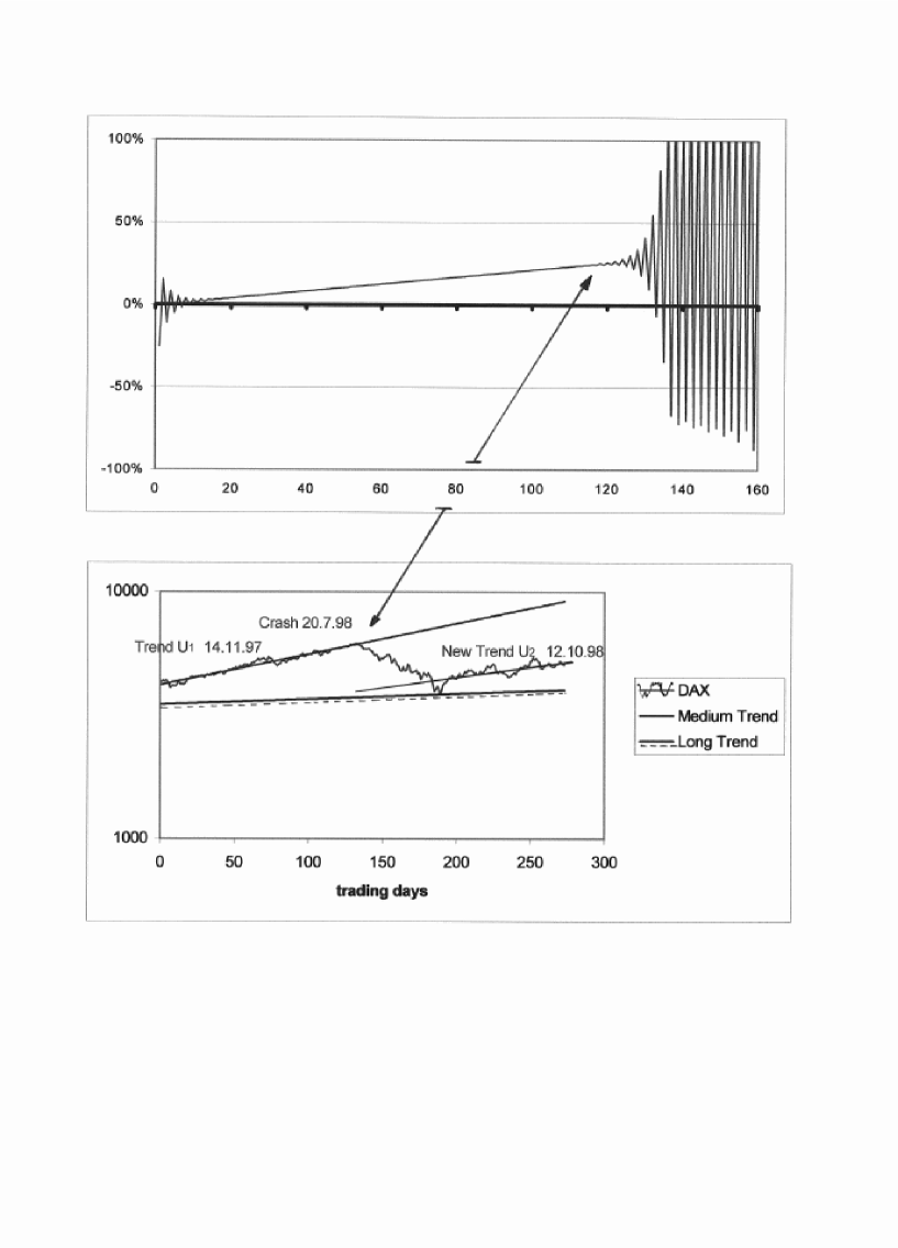
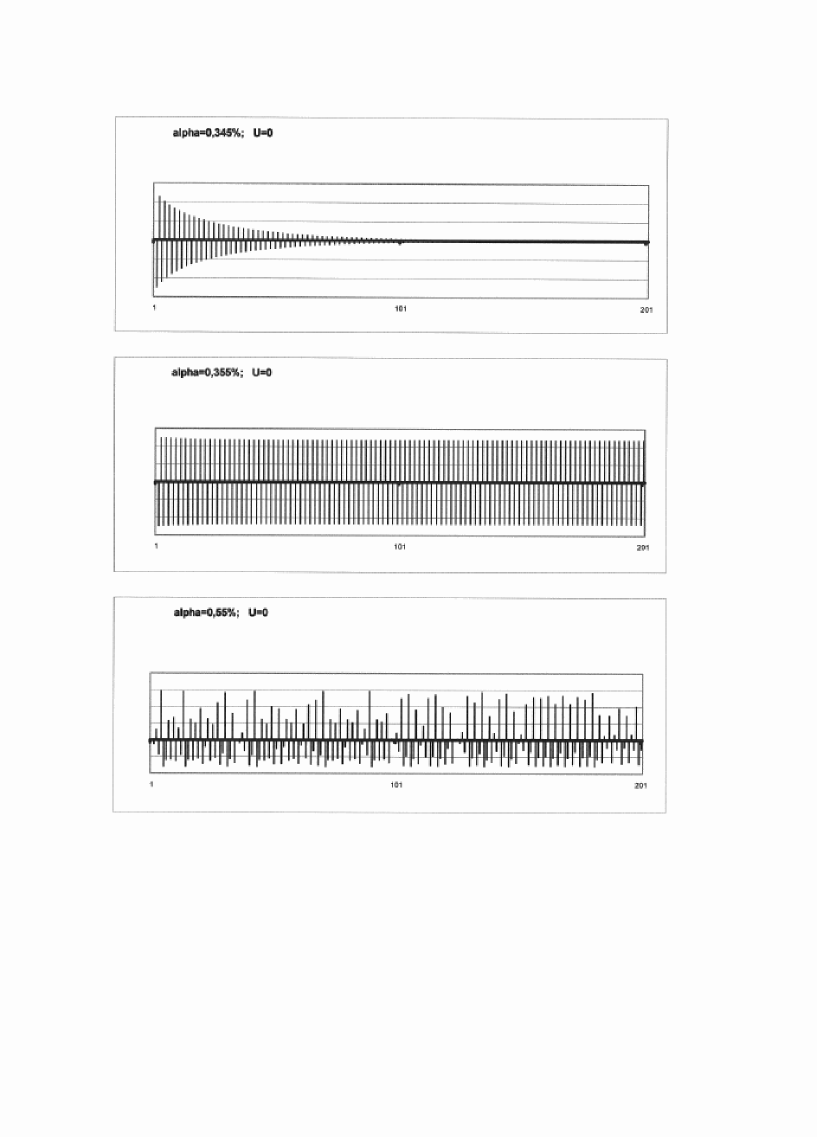
Figure 4: Model behavior of $\Delta i_{n}$ for different parameters $\alpha$

References

- [1] C.Davidson, “The New Science”, 1st International Conference on High Frequency Data in Finance, March 29-31, 1995, Zurich
- [2] G.Caldarelli, M.Marsili and Y.-C. Zhang, “A Prototype Model of Stock Exchange”, cond-math/9709118, SISSA Ref 22/97/CM, 1997
- [3] B.Mandelbrot, Jour. of Business of the Chicago University, 39, p. 242, (1966); dt. 40, p. 393, (1967)
- [4] A.Johansen and D.Sornette, “Critical Crashes”, Risk, v.12, No. 1, p.91, (1999)
- [5] K.Illinski, “Critical Crashes?”, Preprint IPHYS-99-5, (1999)
- [6] J.Agyris, G.Faust, M.Haase, “Die Erforschung des Chaos”, Vieweg, (1995)
- [7] B.Mandelbrot, “Fractals and Scaling in Finance”, Springer, (1997)
- [8] J.D.Farmer, “Market force, ecology and evolution”, Preprint adap-org/9812005, (1998)
- [9] J.-P.Bouchaud and R.Cont, “A Langevin Approach to Stock Market Fluctuations and Crashes”, Preprint cond-mat/98012379, (1998)
- [10] C.Busshaus and H.Rieger, “A Prognosis Oriented Microscopic Stock Market Model”, Preprint cond-mat/9903079, (1999)
-
[11]
T.Hogg, B.A.Huberman and M.Youssefmir, “The Instability of
Markets”, Preprint adap-org/9507002, (1995)
T.Hogg, B.A.Huberman and M.Youssefmir, “Bubbles and Market Crashes”, Preprint adap-org/9409001, (1994)