Non-Separable Halo Bias from High-Redshift Galaxy Clustering

Abstract

The halo model provides a powerful framework for interpreting galaxy clustering by linking the spatial distribution of dark matter haloes to the underlying matter distribution. A key assumption within the linear bias approximation of the halo model is that the halo bias between two halo populations is a separable function of the mass of each population. In this work, we test the validity of the separable bias approximation on quasi-linear scales using both simulations and observational data. Unlike previous studies, we explicitly disentangle the effects of scale dependence of the bias to assess the robustness of bias separability across a broad range of halo masses and redshifts. In particular, we define a separability function based on halo or galaxy cross-correlations to quantify deviations from halo bias separability, and measure it from N-body simulations. We find significant departures from separability on quasi-linear scales ($\sim 1\text{--}5\,\mathrm{Mpc}$) at high redshifts ($z\geq 3$), leading to enhancements in halo cross-correlations by up to a factor of 2 – or even higher. In contrast, deviations at low redshifts remain modest. Additionally, using high-redshift ($z\sim 3.6$) galaxy samples, we detect deviations from bias separability that closely align with simulation predictions. The breakdown of the separable bias approximation on quasi-linear scales at high redshifts underscore the importance to account for non-separability in models of the galaxy–halo connection in this regime. Furthermore, these results highlight the potential of high-redshift galaxy cross-correlations as a probe for improving the galaxy-halo connection from upcoming large-scale surveys.

1 Introduction

In hierarchical theory of structure formation, the gravitationally collapsed dark matter haloes provide potential wells within which galaxies subsequently form and evolve (White & Rees, 1978). The spatial clustering of galaxies, as measured by their correlation functions, traces the underlying large-scale structure of the Universe and carries crucial information about the processes governing cosmic structure formation. Clustering measurements, when interpreted within the framework of a theoretical model, serve as a powerful probe to refine models of galaxy-halo connections and galaxy formation (Seljak, 2000; Scoccimarro et al., 2001; Bullock et al., 2002; Berlind & Weinberg, 2002; Kravtsov et al., 2004; Zheng et al., 2005; Lee et al., 2009; Zehavi et al., 2011; Harikane et al., 2018; Okumura et al., 2021; Chaurasiya et al., 2024; Yuan et al., 2024; Shuntov et al., 2025). In addition, they impose stringent limits on the growth of structures over cosmic time (Yang et al., 2003; Conroy et al., 2006; Jose et al., 2013a; Jose et al., 2013b; Park et al., 2016; Bhowmick et al., 2018; Jiménez et al., 2019; Pei et al., 2024), and constrain cosmological parameters (Tinker et al., 2012; Alam et al., 2017; Ivanov et al., 2020; Abbott et al., 2022; Valogiannis et al., 2024; Pellejero Ibáñez et al., 2024) and beyond $\Lambda$CDM models (Moretti et al., 2023; Gsponer et al., 2024; Hahn et al., 2024). Current and upcoming large-scale surveys measure galaxy and halo clustering across a broad range of redshifts and galaxy luminosities with unprecedented accuracy, advancing a new era of precision cosmology (LSST Dark Energy Science Collaboration, 2012; DESI Collaboration et al., 2016; Euclid Collaboration et al., 2020; Dalmasso et al., 2024).

The correlation functions of dark matter haloes and galaxies are interpreted within the framework of the halo model of large-scale structure (Cooray & Sheth, 2002). In this model, galaxy clustering arises from two distinct components: the one-halo term, which accounts for clustering within individual haloes, and the two-halo term, which describes clustering between galaxies residing in different haloes. The one-halo term dominates on small scales, where clustering occurs within typical dark matter haloes, whereas the two-halo term is due to the clustering of galaxies in distinct haloes and is important on larger scales. A key quantity for calculating the two-halo term is the halo bias, which quantifies the relationship between the spatial distribution of dark matter haloes and the underlying density fluctuations (Kaiser, 1984; Mo & White, 1996). The halo bias is typically calibrated using gravity-only N-body simulations, where physically motivated empirical fitting functions provide accurate approximations across different cosmologies, as theoretical predictions remain challenging (e.g., Sheth & Tormen 1999; Tinker et al. 2005).

A widely adopted assumption within the halo model is the scale-independent linear halo bias approximation, which applies on large scales (Mo & White, 1996). Under this approximation, the halo correlation function is proportional to the matter correlation function, with the proportionality factor given by the square of the scale-independent bias factor (Mo & White, 1996). This approximation has been shown to agree well with results from N-body simulations and has proven effective in modelling low redshift galaxy clustering on large scales (Zheng et al., 2005; Zehavi et al., 2011).

On quasi-linear scales, which are a few times larger than the typical sizes of dark matter haloes, the linear bias approximation often underpredicts the clustering strength. This discrepancy, in the simplest approach, can be reduced by incorporating nonlinear matter power spectrum derived from N-body simulations into the halo model (e.g., Smith et al. 2003). However, this alone is not sufficient. At low redshifts, where the scale dependence of halo bias on quasi-linear scales is relatively small (typically around ten percent), scale-dependent expressions for halo bias are fine-tuned using N-body simulations and incorporated into the halo model (Tinker et al., 2005; Smith et al., 2007; van den Bosch et al., 2013). At high redshifts, theoretical models and simulations reveal a strong scale dependence of the halo bias, resulting in a significant enhancement of clustering on quasi-linear scales (Scannapieco & Barkana, 2002; Barkana, 2007; Reed et al., 2007). This effect, which amplifies galaxy clustering by an order of magnitude on quasi-linear scales, has been calibrated using simulations (Jose et al., 2016) and is essential for accurately interpreting the high redshift galaxy clustering at $z\geq 3$ on quasi-linear scales (Jose et al., 2017; Harikane et al., 2022).

Another key premise of the linear bias approximation is that the halo bias between two halo populations can be expressed as a separable function of the mass of each population (Scoccimarro et al., 2001; Smith et al., 2007, 2011; Schneider et al., 2012). The approximation of bias separability is often adopted in the halo model, as it simplifies the analysis of two-halo clustering (Smith et al., 2007). Incorporating the non-linear matter power spectrum and the scale-dependent halo bias into this framework effectively reproduces observed galaxy clustering across a wide range of redshifts and on large and quasi-linear scales (Zehavi et al., 2005, 2011; van den Bosch et al., 2013; Jose et al., 2017).

Mead & Verde (2021) introduced a beyond-linear bias framework within the halo model, incorporating both the non-separability and scale dependence of halo bias without explicitly disentangling the two effects. Independently, earlier theoretical work by Scannapieco & Barkana (2002) had already indicated that halo bias is not separable at very high redshifts ($z\gtrsim 6$), highlighting the need for more general approaches. A number of subsequent studies have adopted the formalism of Mead & Verde (2021) to interpret galaxy clustering data within the halo model (Mahony et al., 2022; Dvornik et al., 2023; Pizzati et al., 2024); however, their primary focus has been on the implications of non-linear bias, rather than isolating the distinct roles of scale dependence and non-separability.

In this work, we investigate the separability of halo bias using both simulations and observational data. Unlike previous studies, we explicitly test the validity of the separability assumption by disentangling it from the scale dependence of bias of a given halo mass. Specifically, we examine this assumption on quasilinear scales using dark matter simulations that span a wide mass range ($5\times 10^{11}\rm M_{\odot}-5\times 10^{13}\rm M_{\odot}$), which host typical galaxies at both low and high redshifts. Additionally, we perform clustering analysis of the observed bright galaxy samples at $z\sim 3.6$. Our goal is to assess the robustness of the separable bias approximation across different redshifts and to determine whether its validity can be tested with current datasets at high redshifts.

This paper is organized as follows. In Section 2, we briefly discuss the halo model under the assumption of non-separability of halo bias. Section 3 introduces the N-body simulations and observational data used in this study, along with the statistical analysis tools employed. In Section 4, we use the halo cross-correlation to assess the validity of the non-separability assumption of the halo bias using simulations, and subsequently apply the same methodology to observational data. The discussion and conclusions are presented in Section 5. We adopt the cosmological parameters from Planck Collaboration et al. (2020a) for all the analysis in this paper.

2 Non-Separable halo bias and halo cross-correlations

We first introduce the scale-dependent, non-linear halo bias framework for describing the clustering of high-redshift dark matter haloes and galaxies. Since measurements from simulations and observations in this work are made in real space, we present our equations accordingly.

The halo bias $b_{\mathrm{hh}}$ for haloes of masses $M_{1}$ and $M_{2}$ separated by a distance $r$ can be defined using the real-space cross-correlation function of haloes, $\xi_{\mathrm{c}}(r,M_{1},M_{2},z)$, and is given by (Cooray & Sheth, 2002; Smith et al., 2007; Mead & Verde, 2021):

$$\xi_{\rm c}(M_{1},M_{2},r,z)=b^{2}_{\rm hh}(M_{1},M_{2},r,z)\xi_{\rm mm}(r,z).$$ (1)

Here $\xi_{\rm mm}(r,z)$ is the linear matter spatial auto-correlation function. The halo cross-correlation quantifies the excess probability, in N-body simulations, of finding a dark matter halo of one mass $M_{1}$ at a given distance from a halo of another mass $M_{2}$, relative to a random distribution, and serves as an important statistic for characterizing the large-scale matter distribution (Peebles, 1980).

Two key assumptions, commonly employed in the standard halo model, significantly simplify the calculations. The first is the assumption that the halo bias is a separable function of masses $M_{1}$ and $M_{2}$ and is expressed as

$$b^{2}_{\rm hh}(M_{1},M_{2},r,z)=b(M_{1},r,z)b(M_{2},r,z),$$ (2)

where the scale-dependent halo bias $b(M,r,z)$ of dark matter haloes with mass $M$ is defined via their spatial auto-correlation function as

$$\xi_{\rm a}(r,M,z)=b^{2}(M,r,z)\xi_{\rm mm}(r,z).$$ (3)

The second assumption is the scale independence of halo bias given by

$$b(M,r,z)=b(M,z).$$ (4)

Both of these approximations hold on sufficiently large scales, where linear perturbation theory provides a highly accurate description of the growth of structures (Mo & White, 1996; Cooray & Sheth, 2002). Under these conditions, Eq. 1 simplifies to

$$\xi_{\rm c}(M_{1},M_{2},r,z)\simeq b(M_{1},z)b(M_{2},z)\xi_{\rm mm}(r,z).$$ (5)

The scale-independent linear halo bias, $b(M,z)$, depends on the "peak height", $\nu(M,z)=\delta_{c}/\sigma(M,z)$, which quantifies the rarity of dark matter haloes (Kaiser, 1984; Mo & White, 1996; Cooray & Sheth, 2002). Here, $\delta_{c}=1.686$ is the critical overdensity for spherical collapse, and $\sigma(M,z)$ is the root-mean-square (rms) linear density fluctuation on the mass scale $M$, defined as

$$\sigma^{2}(M,z)=\sigma^{2}(R,z)=\int_{0}^{\infty}\frac{dk}{2\pi^{2}}k^{2}P_{\rm lin}(k,z)W^{2}(k,R),$$ (6)

where $R$ is the comoving radius of a sphere enclosing the mass $M$, $W(k,R)$ is the Fourier transform of the spherical top-hat window function, and $P_{\rm lin}(k,z)$ is the linear matter power spectrum (Peebles, 1980).

Among these two assumptions, the scale dependence of halo bias has been more extensively studied using analytic models and N-body simulations. Several alternative models have been developed to better describe how halo bias varies with scale, particularly on quasi-linear scales ranging from approximately 0.5 Mpc to a few Mpc. We therefore briefly discuss this aspect before returning to the validity assumption of separability of bias.

Theoretical and observational efforts have shown that halo bias exhibits pronounced scale dependence on quasi-linear scales—those larger than typical halo sizes (Scannapieco & Barkana, 2002; Iliev et al., 2003; Tinker et al., 2005; Van Den Bosch et al., 2007; Barkana, 2007; Reed et al., 2007; Jose et al., 2016; Jose et al., 2017; Harikane et al., 2022). At low redshifts, this effect leads to a modest increase in the correlation function, typically by a few tens of percent (Tinker et al., 2005). On the other hand, at high redshifts, it can significantly amplify halo clustering (Jose et al., 2016). For rare haloes with masses exceeding $10^{12}\rm M_{\odot}$ at $z\geq 3$, the bias becomes strongly scale-dependent, leading to a correlation function that can be up to an order of magnitude higher on quasi-linear scales than predicted by the linear bias model.

The assumption of separable halo bias, as expressed in Eq. 2, has been more widely adopted than scale-independence of the bias in analytic models of galaxy clustering (Smith et al., 2007, 2011; Lapi & Danese, 2021). While computationally simple and often sufficiently accurate, this simplification has recently been revisited. In particular, Mead & Verde (2021) proposed an alternative beyond linear bias framework where the halo bias is scale-dependent and no longer a separable function of $M_{1}$ and $M_{2}$. In this case, the halo power spectrum is defined as,

$$P(M_{1},M_{2},k,z) =b(M_{1},z)b(M_{2},z)P_{\rm lin}(k,z)$$ (7)

$$\quad\times\left[1+\beta_{\text{NL}}(M_{1},M_{2},k,z)\right],$$

The term $\beta_{\text{NL}}(M_{1},M_{2},k,z)$ is a non-separable function of $M_{1}$ and $M_{2}$ that also incorporates the scale dependence of halo bias. On large scales, where the linear bias approximation remains valid, $1+\beta_{\text{NL}}$ approaches unity.

At $z\sim 0$, for haloes with masses in the range of $10^{11}-10^{13}M_{\odot}$, $\beta_{\text{NL}}$ enhances cross-correlations by 10-20%. Following (Mead & Verde, 2021), a number of studies have incorporated this non-separable and scale-dependent bias into the halo model to understand the observed clustering of galaxies at low redshifts (Mahony et al., 2022; Dvornik et al., 2023) and analyze the quasar correlation functions at $z\sim 6$ (Pizzati et al., 2024).

The definition of $\beta_{\text{NL}}(M_{1},M_{2},k,z)$ by Eq. 7 does not explicitly separate the scale-dependence from the non-separability of the halo bias. Therefore, in order to assess whether the assumption of bias function separability remains valid on quasi-linear scales, we must disentangle the effects of separability from the inherent scale dependence of the bias of halo of mass $M$. To achieve this, we introduce a real space halo bias separability function $s(M_{1},M_{2},r,z)=1+\alpha(M_{1},M_{2},r,z)$, such that

$$\xi_{\rm c}(M_{1},M_{2},z,r) =b(M_{1},r,z)\,b(M_{2},r,z)\xi_{\rm mm}^{\rm lin}(r)\,$$ (8)

$$\quad\times\left[1+\alpha(M_{1},M_{2},r,z)\right].$$

Note that while $s$ retains a dependence on scale, the explicit scale dependence associated with the halo bias at each mass, $b(M,r,z)$, has been factored out by this definition. The separability function $s(M_{1},M_{2},r)$ can be estimated from cosmological N-body simulations as

$$s(M_{1},M_{2},r,z)=\frac{\xi_{\rm c}(M_{1},M_{2},r,z)}{\sqrt{\xi_{\rm a}(M_{1},r,z)\,\xi_{\rm a}(M_{2},r,z)}}.$$ (9)

On sufficiently large scales, where the linear bias approximation is valid, the function $s(M_{1},M_{2},r,z)$ is expected to approach unity, similar to the behaviour of $1+\beta_{\text{NL}}$ and in this case the bias is a separable function of $M_{1}$ and $M_{2}$. Also, by definition, $s(M_{1},M_{2},r,z)$ also tends to unity when the two halo masses become equal (as $M_{1}\to M_{2}$), and this holds across all spatial scales. Thus, $s$ is sensitive primarily to the non-separability of halo bias function. In contrast, $1+\beta_{\text{NL}}$, which also accounts for the scale dependence of bias, deviates from unity even as $M_{1}\to M_{2}$, particularly on quasi-linear scales. Therefore, the function $s(M_{1},M_{2},z,r)$ provides a reliable and more direct probe for isolating the separability of halo bias function, independently of the scale dependence in $b(r,M,z)$.

Furthermore, the estimation of $\beta_{\text{NL}}$ from observations requires knowledge of the linear matter correlation function, which in turn depends on the assumption of a specific set of cosmological parameters. In contrast, the function $s$ can, in principle, be measured directly from observations, as it requires only halo–halo (or galaxy–galaxy) cross- and auto-correlation functions for its computation. This make $s$ less reliant on cosmological modelling assumptions, enabling for a more straightforward comparison between observations and simulations.

2.1 How rare are high-z galaxy-hosting haloes?

Figure 1: Top panel: Halo masses corresponding to various values of $\nu$ as a function of redshift. Bottom panel: The total number of dark matter haloes in unit logarithmic mass interval in the sky, per unit redshift interval, with a given $\nu$, as a function of redshift.

It is important to note that the high-redshift galaxy populations used in this study are statistically distinct from their low-redshift counterparts in terms of their host halo properties. The galaxies analysed here have halo masses ranging from approximately $5\times 10^{11}$ to a few times $10^{13}\,\rm M_{\odot}$ (Harikane et al., 2022). At low redshift $(z\sim 0)$, emission-line galaxies and luminous red galaxies (LRGs) from SDSS and DESI, which are typically not associated with clusters or groups, have comparable halo masses (Masaki et al., 2013; van Uitert et al., 2015; Gao et al., 2023; Berti et al., 2023).

Although the halo masses of high-redshift galaxies are slightly smaller than their low-redshift counterparts, high-redshift haloes are statistically much rarer, as they form from high-$\sigma$ fluctuations. Using Eq. 6 and $\nu=\delta_{c}/\sigma$, we obtain the masses of haloes collapsing from $2.5$, $3$, and $4\sigma$ fluctuations as a function of redshift, which we show in the top panel of Fig. 1. It is evident that, for a given $\nu$, the halo mass is lower at high $z$, which means that haloes of a given mass are much rarer at high redshifts. For example, $10^{13}\,\rm M_{\odot}$ haloes at $z\sim 4$, which collapse from $4\sigma$ fluctuations, are as rare as superclusters at $z\sim 0$.

In the lower panel of Fig. 1, we also show the total number of dark matter haloes per unit logarithmic mass and redshift in the sky, corresponding to a given $\nu$, obtained from the Tinker et al. (2005) halo mass function. Clearly, for a given $\nu$, this number increases with redshift. For example, at $z\sim 4$, there are about a million haloes with a mass of $10^{13}\,\rm M_{\odot}$ per unit logarithmic mass interval and unit redshift, compared to only a few hundred objects with similar $\nu$ ($M\sim 5\times 10^{15}\,\rm M_{\odot}$) at $z\sim 0$. These larger samples of rare, high-redshift haloes enable detailed statistical analyses of their properties. As tracers of the extreme tail of the halo mass distribution, their statistical behaviour is expected to differ significantly from that of their low-redshift counterparts.

3 The data and Measurements

In this section, we provide an overview of the N-body simulations and observational data used in our study to probe the impact of non-separable bias on quasi-linear scale clustering of dark matter haloes and galaxies. Additionally, we describe the statistical estimators employed for measuring halo and galaxy correlation functions, along with the methods used to quantify uncertainties.

3.1 The Abacus N-body Simulations

We use the AbacusSummit suite of N-body simulations, a large volume, high-accuracy and high-resolution dataset designed to support large-scale structure studies in the era of next-generation surveys (Maksimova et al., 2021). It consists of over 150 simulations covering 97 cosmological models. These simulations were produced using Abacus, a GPU-optimized N-body code that employs the static multipole mesh method to efficiently compute gravitational interactions (Garrison et al., 2021; Hadzhiyska et al., 2022). They enable precise measurements of halo auto- and cross-correlations, particularly for very massive dark matter haloes at high redshifts, which are required in this study.

To compute halo correlations, we use simulations based on the Planck 2018 baseline $\Lambda$CDM cosmology (Planck Collaboration et al., 2020b). In particular two simulation volumes are used: (i) huge simulation, with $8640^{3}$ particles in 7.5 $h^{-1}$ Gpc box, with a particle mass resolution of $5\times 10^{10}h^{-1}\rm M_{\odot}$, and (ii) base simulation, with $6912^{3}$ particles in 2$h^{-1}$Gpc box, with a particle mass resolution of $2\times 10^{9}h^{-1}\rm M_{\odot}$(Maksimova et al., 2021). Dark matter haloes in these simulations are identified using the CompaSO algorithm  (Hadzhiyska et al., 2022), which assigns halo masses based on spherical overdensity criteria. We adopt $M_{200}$, the mass enclosed within a region of 200 times the critical density of the universe, as our halo mass definition.

3.2 The HSC-SSP observations

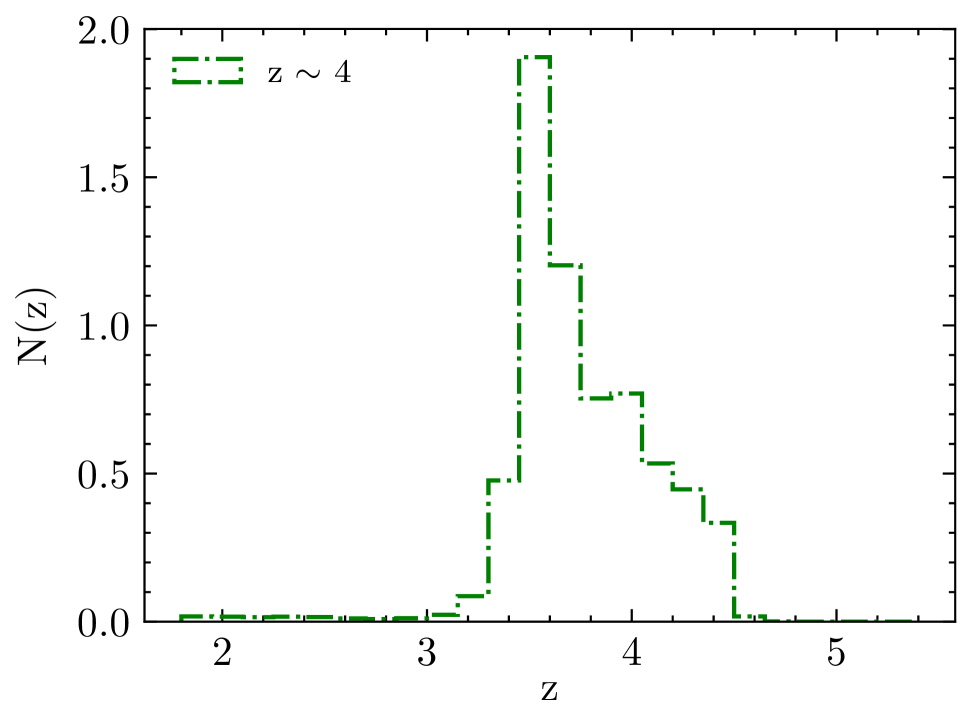
Figure 2: Normalized redshift distribution of g-dropouts with $20<\rm m_{\rm UV}<24.5$ from HSC-SSP wide survey.

Our analysis employs galaxy catalogues from the third public data release (PDR3) of HSC-SSP, as presented in Aihara et al. (2022) (see Aihara et al. 2018, 2019 for eariler data releases). The HSC-SSP survey spans three layers —wide ($\sim$ 670 deg²), deep ($\sim$ 28 deg²), and ultra-deep ($\sim$ 3 deg²). In this work, we utilize wide layer galaxies from the Spring and Autumn fields covering approximately 600 deg². Photometric data from the five HSC broad-band filters ($g$, $r$, $i$, $z$, $y$) (Kawanomoto et al., 2018) are processed through the hscPipe reduction pipeline (Bosch et al., 2018) to generate the galaxy catalogues. These catalogues are used to measure the auto- and cross-correlations of magnitude-selected Lyman Break Galaxy (LBG) g-dropout samples which are identified via the Lyman break technique which traces the redshifted Lyman-limit break (at rest-frame wavelength of 912 $\AA$) in the galaxy spectral energy distributions (Steidel et al., 1996; Giavalisco, 2002).

As in Harikane et al. (2022), we select galaxies with signal-to-noise ratios greater than $5$ within $1.5^{\prime\prime}$ diameter apertures and apply the masks, threshold values, and flags described in Section 2 and Table 2 of Harikane et al. (2022) to exclude galaxies compromised by pixel issues, cosmic rays, and bright source haloes (Coupon et al., 2018). The color selection for dropout galaxies is then applied to the convolved fluxes within $2^{\prime\prime}$ diameter apertures after aperture correction, specifically for g-dropouts as outlined in Ono et al. (2018), Toshikawa et al. (2018), and Harikane et al. (2018).

$$(g-r>1.0)\Lambda(r-i<1.0)\Lambda(g-r>1.5(r-i)+0.8).$$ (10)

Once the galaxies are color-selected, the fixed $2^{\prime\prime}$ diameter aperture magnitude after aperture correction is used as the total magnitude in all filters Harikane et al. (2022). The UV magnitude ($\text{m}_{\text{UV}}$) for the g-dropouts is the $i$-band magnitude, whose central wavelength is the nearest to the rest frame wavelength of $\lambda\approx 1500$ Å.

3.3 Removal of low-z interlopers

Low-z interlopers satisfying the above color-selection criteria contaminate the HSC-SSP. In order to remove these, we utilize the photometric redshifts (photo-z) of the galaxies as given by PDR3, derived using the empirical photometric redshift fitting code DEmP (Hsieh & Yee, 2014; Tanaka et al., 2018). The DEmP utilizes template data of galaxies with spectroscopic redshifts from the literature to obtain a polynomial fit to the probability distribution function (PDF) of photo-z of galaxies. This fit is then used to derive the best-fit value, which we adopt in this work.

As in Toshikawa et al. (2024), the low redshift interlopers are also removed from the g-dropouts, by selecting g-dropout galaxies with the upper bound on the 95 percent confidence interval of the photo-z greater than $2.8$. We show in Fig. 2, the distribution of the best-fit photo-z, $N(z)$, of the g-dropouts with $20<\rm m_{\rm UV}<24.5$. This constitutes our final sample, which will be used for clustering analysis. The median redshift of the final sample is $z_{m}\sim 3.6$.

3.4 The 2-point auto and cross-correlations

In this section, we discuss how to compute the angular or spatial two-point auto- and cross-correlations of galaxy or halo samples discussed in previous sections. The angular two-point auto-correlation is estimated using the well-known Landy-Szalay estimator Landy & Szalay (1993) as

$$\omega_{\rm a}(\theta)=\frac{\langle DD(\theta)\rangle-\langle 2DR(\theta)\rangle+\langle RR(\theta)\rangle}{\langle RR(\theta)\rangle}\,$$ (11)

where $\langle DD(\theta)\rangle$, $\langle DR(\theta)\rangle$, and $\langle RR(\theta)\rangle$ are the numbers of galaxy-galaxy, galaxy-random, and random-random pairs at a pair separation angle $\theta$, normalized by the total number of pairs. A random catalogue that accounts for masked regions and edge effects within the survey area is essential for computing the number of random pairs. In this work, we have used the random catalogues supplied by Aihara et al. (2022) (see also Coupon et al. 2018), with a surface density of 100 points per arcmin².

To study the clustering between two distinct galaxy samples (sample 1 and 2), we compute their two-point angular cross-correlation function using

$$\omega_{\rm c}(\theta)=\frac{\langle D_{1}D_{2}(\theta)\rangle-\langle D_{1}R(\theta)\rangle-\langle D_{2}R(\theta)\rangle+\langle RR(\theta)\rangle}{\langle RR(\theta)\rangle}\,,$$ (12)

where $\langle D_{1}D_{2}(\theta)\rangle$ is the normalized number of galaxy-galaxy pairs between galaxy sample 1 and 2 at a pair separation angle $\theta$. Similarly, $\langle D_{1}R(\theta)\rangle$ is the number of galaxy-random pairs between galaxy sample 1 and random catalogue. In this work, we obtain both samples by selecting galaxies from two non-overlapping magnitude bins.

The spatial auto-correlation and cross-correlation functions of dark matter haloes are computed similarly using Eqs. 11 and 12, but the pair count is measured as a function of real-space separation $r$ of haloes instead of their angular separation $\theta$. Thus, in this case, $\langle DD(r)\rangle$, $\langle DR(r)\rangle$, and $\langle RR(r)\rangle$ correspond to the halo-halo, halo-random, and random-random pair counts, respectively.

3.4.1 Statistical Uncertainties

The statistical errors of the angular correlation function are estimated using the Jackknife resampling method (Norberg et al., 2009) with Jackknife regions of size $\sim 5$ square degrees. The Jackknife covariance matrix is then

$$C_{ij}=\frac{N-1}{N}\sum_{k=1}^{N}(\omega^{k}(\theta_{i})-\bar{\omega}(\theta_{i}))(\omega^{k}(\theta_{j})-\bar{\omega}(\theta_{j}))$$ (13)

where $\omega^{k}(\theta_{i})$ is the angular correlation function at $\theta$=$\theta_{i}$ from the $k^{th}$ Jackknife region and $\bar{\omega}$ is the average correlation function of a total of $N$ Jackknife regions (Scranton et al., 2002; Zehavi et al., 2005).

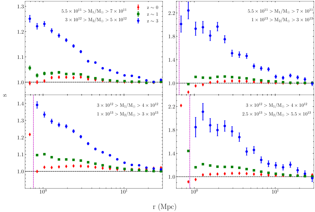
Figure 3: The halo bias separability function as a function of the halo separation at the redshifts 0 (red diamonds), 1 (green squares) and 3 (blue circles), for halo samples in different mass bins, as indicated in the legend. The measurements in upper and lower panels are respectively from the base and the huge simulations.

Magnitude ($m_{\rm UV}$) bins	20-23.9	24.2-24.5	20-23.75	24.1-24.5
Number of galaxies	19,306	99,943	11,034	1,17,591
Effective bias $({\text{b}_{\text{eff}}})$	9.46±0.69	5.06±0.19	11.8±1.2	5.13±0.17
Effective mass $({\text{M}_{\text{eff}}/\text{M}_{\odot}})$	$9.86\begin{subarray}{c}+2.1\\ -1.9\end{subarray}\times 10^{12}$	$1.39\begin{subarray}{c}+0.19\\ -0.17\end{subarray}\times 10^{12}$	$1.8\begin{subarray}{c}+0.53\\ -0.46\end{subarray}\times 10^{13}$	$1.46\begin{subarray}{c}+0.17\\ -0.16\end{subarray}\times 10^{12}$

Table 1: Number of g-drop galaxies in different magnitude subsamples, and the corresponding effective bias and halo mass.

4 Result and Discussion

4.1 Non-separable bias from Simulations

In this section, we present the halo bias separability function, measured from N-body simulations at different redshifts. To measure $s(M_{1},M_{2},r,z)$, we require two halo samples with different masses. Therefore, we select haloes from the simulation in a pair of distinct mass bins; the first bin, denoted by $[M_{1}]$, is defined as $M_{1}^{\text{start}}\leq M_{1}<M_{1}^{\text{end}}$. The average mass of the bin $[M_{1}]$ is then given $M_{1}^{\text{av}}=(M_{1}^{\text{start}}+M_{1}^{\text{end}})/2$. The corresponding average virial radius is given by,

$$r_{1}^{\text{av}}=\dfrac{3M_{1}^{\text{av}}}{4\pi\rho_{\text{cric}}\Delta},$$ (14)

where $\rho_{\text{cric}}$ is the critical density of the Universe and $\Delta=200$. Similarly, for the second sample $[M_{2}]$, we have $M_{2}^{\text{start}}\leq M_{2}<M_{2}^{\text{end}}$. The halo masses in the two samples are chosen to be non-overlapping.

We then estimate the auto-correlation function, $\xi_{\text{hh}}([M],r,z)$, of dark matter haloes within each mass bin, as well as the cross-correlation, $\xi_{\text{hh}}([M_{1}],[M_{2}],r,z)$, between haloes in the two bins. These correlation functions are used to compute the separability function $s$ (as defined in Eq. 9). A deviation of $s$ from unity quantifies the extent to which halo bias is non-separable across the selected mass bins.

Fig. 3 shows the separability function $s$ measured for different pairs of halo mass bins at $z\sim 0$, 1, and 3, as a function of separation $r$. Each panel presents the evolution of $s$ with redshift for a fixed pair of mass bins, which are specified in the legend. For example, in the first panel, $s$ is measured using halo mass bins defined by $5.5\times 10^{11}<M_{1}/M_{\odot}<7\times 10^{11}$ and $3\times 10^{12}<M_{2}/M_{\odot}<5\times 10^{12}$. We use relatively wider mass bins to ensure that each sample contains a sufficient number of haloes for a statistically robust measurement of $s$. The vertical lines in each panel indicate a conservative upper limit on the halo exclusion scale, $r_{1}+r_{2}$. Below this scale, halo exclusion effects can be important; therefore, we do not analyze the behavior of $s$ in that regime.

We first note that for all pairs of mass bins, $s$ departs from unity on quasi-linear scales (approximately $1\text{--}5$ Mpc), demonstrating that halo bias is a non-separable function of $M_{1}$ and $M_{2}$ in this regime. On most of these scales, and at all redshifts, $s$ exceeds unity, which implies an enhanced probability of finding haloes of masses $M_{1}$ and $M_{2}$ at a separation $r$ relative to the expectation from Eqs. 1 and 2. However, at $z\sim 0$ and on scales around $1\mathrm{Mpc}$, $s$ falls below one, suggesting a reduced likelihood of such halo pairs being found at that distance.

The extent to which the separability factor differs from unity varies significantly with redshift. At low redshifts $(z\sim 0)$, this difference remains relatively modest—at most $\sim 10\%$ for the mass ranges considered here. At an intermediate redshift of $z\sim 1$, the maximum deviation increases to $\sim 20\%$, indicating a stronger departure from separability. In contrast, at higher redshifts, the shift from unity becomes substantially more pronounced. At $z\sim 3$, $s$ deviates considerably from unity, reaching values as high as $\sim 2.2$ (see the right panels of Fig. 3). This strong deviation clearly indicates that the assumption of separable halo bias breaks down at high redshifts ($z\gtrsim 3$) on quasi-linear scales. The excess of $s$ over unity results in an enhancement of the cross-correlation function by the same factor.

The scale up to which $s$ departs from unity also exhibits a redshift dependence. At $z\sim 0$, non-separable bias remains significant up to scales of approximately $5-10\,\mathrm{Mpc}$, beyond which $s$ approaches unity, indicating that the halo bias becomes effectively separable. In contrast, for halo samples of similar mass at $z\sim 3$, the deviation from unity persists even on scales of about $20\,\mathrm{Mpc}$. This demonstrates that the scale over which the bias is non-separable increases with redshift for given $M_{1}$ and $M_{2}$.

The separability function $s$ also depends strongly on both the masses of the halo samples and the mass separation between them. At a fixed redshift, the deviation of $s$ from unity becomes more pronounced for haloes with higher masses and for pairs of samples drawn from increasingly separated mass bins. In particular, at $z\sim 3$, for the most massive haloes (shown in the last panel of Fig. 3), the assumption of separability breaks down even on scales as large as $25\,\mathrm{Mpc}$.

As discussed in Section 2, massive haloes at high redshift collapse from rare $3\text{--}4\sigma$ fluctuations; hence, their distribution may differ significantly from that of galaxy-hosting halos of similar mass at lower redshifts. Correspondingly, the separability function deviates progressively more from unity, increasing from a modest 10% at low redshift ($z\sim 0$ or $1$) to well over 100% at $z=3$. The strong high-$z$ signals of the separability function present a unique opportunity to measure it from high-redshift galaxy surveys, which we explore in the next section.

4.2 Non-separable bias from Galaxy Cross-Correlation Functions

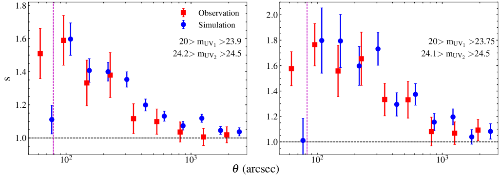
Figure 4: The bias separability function derived using HSC-SSP galaxy samples at $z\sim 3.6$ (red squares) and Abacus Simulation halo catalogues at $z\sim 3$ (blue circles).

In this section, we present the measurements for the bias separability function for galaxy samples from the HSC-SSP survey at $z\sim 3.6$, as a function of the angular scale $\theta$. These high redshift galaxy populations from the HSC-SSP survey are typically associated with halo masses exceeding $10^{12}{\rm M}_{\odot}$ (Harikane et al., 2022), placing them in a regime where non-separability is expected to be very prominent. Moreover, the large number of galaxies from the 600 deg² wide field makes this dataset particularly well-suited for measuring $s$ with high statistical significance.

In order to measure $s$, we divide the galaxy sample into two UV magnitude bins, denoted by $[\rm m_{\text{uv1}}]$ and $[\rm m_{\text{uv2}}]$. Since UV luminosity traces halo mass, this binning approximately acts as a proxy for galaxy selection based on halo mass. We then measure the angular auto-correlation of galaxies within each magnitude bin and the angular cross-correlation between galaxies in these two bins. Using these measurements, we calculate the separability function as

$$s([\rm m_{\text{uv1}}],[\rm m_{\text{uv2}}],\theta,z)=\frac{\omega_{\rm c}([\rm m_{\text{uv1}}],[\rm m_{\text{uv2}}],\theta,z)}{\sqrt{\omega_{\rm a}([\rm m_{\text{uv1}}],\theta,z)\,\omega_{\rm a}([\rm m_{\text{uv2}}],\theta,z)}}.$$ (15)

In Figure 4, we present the measured separability function $s$ (red squares) for two independent cases, each based on a different pair of non-overlapping UV magnitude bins. In the first case, shown in the left panel, the bins are defined as $20<\rm m_{\text{uv1}}\leq 23.9$ and $24.2<\rm m_{\text{uv2}}\leq 24.5$. In the second case, shown in the right panel, the magnitude gap between bins is slightly wider, with the bins given by $20<\rm m_{\text{uv1}}\leq 23.75$ and $24.1<\rm m_{\text{uv2}}\leq 24.5$. The uncertainties in the measurements are estimated using the Jackknife resampling method described in Section 3.4.1. The number of galaxies in each magnitude bin that make up the samples is tabulated in Table 1. It is clear from the figure that $s$ exceeds unity even for $\theta\lesssim 1500^{\prime\prime}$ (corresponding to scales as large as 11 Mpc) and the deviations increase with decreasing scale. The vertical line in each panel indicates an effective halo-exclusion scale, calculated as described in Section 4.1, using the virial radius given in Eq. 14, with the average mass replaced by the effective mass of the samples. The procedure for computing the effective mass is described later in this section.

At smaller angular scales, the deviation of $s$ from unity is consistently larger in the right panel of the figure. For instance, at $\theta\sim 100^{\prime\prime}$, $s$ reaches a value of 1.8 in the right panel, compared to approximately 1.6 in the left. This difference may result from the larger separation in UV magnitude between the bins used in the right panel. The scale dependence of $s$ is consistent with the trends seen in the $N$-body simulations presented in Section 4.1 and provides compelling evidence for the non-separable halo bias.

We quantify the deviation of $s$ from unity by performing the $\chi^{2}$ goodness-of-fit test, treating $s=1$ as the null hypothesis (a constant function of $\theta$). For the left and right samples shown in Figure 4, the $\chi^{2}$ values are $78.3$ and $125.5$, corresponding to p-values of $1.4\times 10^{-10}$ and $1.6\times 10^{-19}$, respectively. These large $\chi^{2}$ values and exceedingly small p-values strongly indicate that the parameter $s$ deviates significantly from unity in the observational data.

In order to compare the observational results for $s$ with those from $N$-body simulations, it is necessary to determine the halo masses corresponding to the galaxy samples used in the measurement. This is often done through a halo-model analysis of galaxy cross-correlations, which is beyond the scope of this work. Instead, we infer the effective halo mass of each observational sample from its measured large-scale bias. The separability function $s$ is then measured from $N$-body simulations for haloes with the same effective mass and compared directly with the observational results for $s$.

To determine the effective mass of the galaxy samples defined by UV magnitude bins, we begin by estimating their large-scale bias using the method described in (Mons & Jose, 2024). This requires computing the linear dark matter spatial correlation function, given by,

$$\xi_{\text{mm}}(r,z)=\dfrac{1}{2\pi^{2}}\int dkP(k,z)\dfrac{\sin(kr)}{kr},$$ (16)

where $P(k,z)$ is the linear matter power spectrum and is computed for Planck cosmology (Planck Collaboration et al., 2020a).

We applied the Limber transformation (Limber, 1953) to $\xi_{\text{mm}}(r)$, using the redshift distribution of the sample galaxies given in Section 3.2 to compute the dark matter angular correlation function $\omega_{\text{mm}}(\theta)$. The galaxy bias as a function of $\theta$ is then estimated for each magnitude-binned sample using its observed angular auto-correlation function as

$$b_{g}^{2}(\theta)=\omega_{\rm a}(\theta)/\omega_{\text{mm}}(\theta).$$ (17)

As in (Mons & Jose, 2024), we find that the bias remains approximately constant over the angular range $100^{\prime\prime}\leq\theta\leq 500^{\prime\prime}$ for all galaxy samples. We therefore define the effective large-scale galaxy bias of the sample as:

$$b_{\text{eff}}=\dfrac{\int\omega_{a}(\theta)\,\theta^{2}\,d\theta}{\int\omega_{\text{mm}}(\theta)\,\theta^{2}\,d\theta},$$ (18)

where the integrals are evaluated over the angular range $\theta=100^{\prime\prime}$ to $500^{\prime\prime}$. The resulting effective bias, $b_{\rm eff}$ is listed in Table 1 for each sample. The errors in the measured galaxy angular correlation functions, determined using the Jackknife method, are propagated to estimate the uncertainties in the effective bias (also given in Table 1).

The relation between halo mass and bias (discussed in Section 3.4) has been well calibrated using $N$-body simulations (e.g., Sheth & Tormen 1999; Tinker et al. 2010). We determine the effective halo mass of the sample, $\rm M_{\text{eff}}$, from its effective large-scale bias, $\rm b_{\text{eff}}$, by applying the halo bias–mass relation of Tinker et al. (2010), propagating the uncertainty in $\rm b_{\text{eff}}$ to estimate the error in $\rm M_{\text{eff}}$. Our estimates of the $\rm M_{\text{eff}}$ of the UV magnitude-binned galaxy samples ($[\rm m_{\text{uv}}]$) used to measure $s$, along with their associated uncertainties, are listed in Table 1. It is worth noting that this effective halo mass may not precisely correspond to the average halo mass of the sample, as derived from a full halo model analysis; nonetheless, it provides a robust and useful approximation.

We next measure $s$ corresponding to the observed galaxy samples directly from simulations. Since $N$-body simulation data are unavailable at the observed redshift of $z=3.6$, we instead use data at $z\sim 3$, the closest available snapshot. To do this, we select haloes from the simulation in mass bins matching the 1-$\sigma$ range of $\rm M_{\text{eff}}$ for each of the two magnitude-binned galaxy samples used in the observational measurement of $s$. For example, the halo mass bin corresponding to the sample with $20\leq\rm m_{\rm UV}<23.9$ and $\rm M_{\rm eff}=9.86\begin{subarray}{c}+2.1\\ -1.9\end{subarray}\times 10^{12}\text{M}_{\odot}$ is defined as $7.96\times 10^{12}\leq M/\text{M}_{\odot}<1.196\times 10^{13}$. The separability function is then computed for both sets of mass-binned samples from simulations, as described in Section 4.1. The results are shown as blue circles in Fig. 4, after converting spatial separations $r$ to angular scales $\theta$ using the angular diameter distance.

Remarkably, the simulation-based measurements are in excellent agreement with the observational results, clearly demonstrating the robustness of the non-separability of the halo bias. This suggests that the bias seperable function may serve as a valuable observational probe in the future for constraining both the astrophysical processes governing galaxy formation at high redshifts and the cosmological parameters.

4.3 Impact of satellite galaxies on the separability function

The observed galaxy sample includes both central and satellite galaxies, whereas our simulation-based measurements of $s$ thus far have considered only dark matter haloes. Central galaxies reside at the centers of haloes, while satellites follow the dark matter distribution around the central galaxy. Therefore, measurements based solely on haloes primarily trace the clustering of central galaxies, without accounting for the contribution of satellites. To assess the impact of satellites, we populate haloes with both the central and the satellite galaxies and re-measure $s$. This enables us to evaluate whether the observed bias separability function remains robust in the presence of satellite galaxies.

To populate dark matter haloes with galaxies, one requires a Halo Occupation Distribution (HOD) model (Cooray & Sheth, 2002), which provides a statistical framework for describing the number of central and satellite galaxies residing in haloes of a given mass. We employ a simple HOD prescription to generate a mock galaxy catalogue from the $N$-body simulations that reflects the observed HSC-SSP galaxy population. For this we have utilized the Abacus Summit huge simulations with a box size of $7500$ Mpc/h.

We begin by assuming a simple scaling relation in which the luminosity of a central galaxy is proportional to its host halo mass ($L=kM$, where $k$ is a constant). Under this assumption, the mean number of central galaxies, $\bar{N}_{c}$, in a sample defined by a luminosity threshold $L_{\rm th}$ follows a step function:

$$\bar{N_{c}}=\Theta(M,M_{\rm th}),$$ (19)

where $L_{\rm th}=kM_{\rm th}$. In this model, all dark matter haloes with mass exceeding $M_{\rm th}$ host a central galaxy with luminosity greater than $L_{\rm th}$, located at the halo center and assigned the same mass as the parent halo (Tinker et al., 2005).

The average number of satellite galaxies in a halo of mass $M$, $\bar{N_{s}}$, is modelled as a power law (Harikane et al., 2022):

$$\bar{N_{s}}=\begin{cases}\left(\dfrac{M-M_{\rm th}}{M_{1}}\right)^{\alpha}&\text{if }M\geq M_{\rm th},\\ 0&\text{if }M<M_{\rm th}.\end{cases}$$ (20)

Following Harikane et al. (2022), we adopt $\alpha=1$. The number of satellite galaxies within a dark matter halo of mass $M$ is drawn from a Poisson distribution with mean $\bar{N}_{s}$. The masses of the satellite galaxies brighter than the luminosity threshold $L_{\rm th}$ are assigned using the subhalo mass function (SHMF), which describes the average number of satellites of mass $M_{s}$ residing within a halo of mass $M$:

$${\rm SHMF}(M_{\rm s}\mid M)=\begin{cases}A\left(\frac{M_{\rm s}}{\gamma M}\right)^{-\beta},\quad&M_{\rm th}\leq M_{\rm s}<M/2,\\ 0,&\text{Otherwise }.\end{cases}$$ (21)

where we adopt $\beta=2$ and $\gamma=0.5$, following Lee et al. (2009) (see also Bosch et al. (2004); Jiang & Van Den Bosch (2016)). Thus, the maximum mass of a satellite galaxy is limited to half the mass of its host halo. The constant $A$ is fixed using the average number of satellites, $N_{s}(M)$. The luminosity of a satellite galaxy is also assumed to be $L_{s}=kM_{\rm s}$. The spatial distribution of satellite galaxies around the central galaxy is modeled using random positions drawn from a Navarro–Frenk–White profile. In the absence of satellites, the catalogue consists solely of central galaxies located at the centers of dark matter haloes with masses above the threshold $M_{\rm th}$.

The HOD parameters $M_{\rm th}$ and $M_{1}$ are chosen so that the resulting galaxy number density $n_{g}$ and satellite fraction $f_{\rm sat}$—defined as the ratio of the number density of satellite galaxies to the total galaxy number density and both computed directly from the simulations — match those of realistic galaxy samples used for measuring $s$. For the catalogues constructed here, we use $M_{\rm th}=3.59\times 10^{12}$ and $M_{1}=2.9\times 10^{13}$ to obtain a galaxy number density of $n_{g}=5\times 10^{-5}\,\mathrm{Mpc}^{-3}$ and a satellite fraction of $f_{\rm sat}=5\%$. For comparison, the number density of samples with a threshold luminosity of 24.5 is $6.1\times 10^{-5}$, while the satellite fraction in the HSC-SSP survey is approximately 2%. (Table 8 of Harikane et al. (2022).

Thus, the final catalogue contains both central and satellite galaxies with $M>M_{\rm th}$. In our model, galaxy luminosity is proportional to halo mass with an arbitrary proportionality constant $k$. Therefore, instead of dividing the catalogue into luminosity/magnitude bins to measure $s$, we bin galaxies directly by mass. While more realistic HOD models treat luminosity as a stochastic function of halo mass, we leave such extensions to future work.

To assess the impact of satellite galaxies on $s$, we first split the full galaxy catalog—including both centrals and satellites—into two mass bins defined by $3\times 10^{12}<M_{1}/M_{\odot}\leq 5\times 10^{12}$ and $2.5\times 10^{13}<M_{2}/M_{\odot}\leq 5.5\times 10^{13}$ , and measured $s([M_{1}],[M_{2}])$ following the procedure described in Section 4.1. We then removed the satellites and recomputed $s$ for the same mass bins.

The results, shown in Figure 5, show that the presence of satellites slightly suppresses the deviation of $s$ from unity, thereby weakening the non-separability signal. Nevertheless, the signal remains clearly visible even with satellites included. This suggests that the observed non-separability is not an artifact introduced by satellite contamination, but a genuine feature of the galaxy distribution. The fact that the signal is even stronger in the absence of satellites further supports the robustness of our main result.

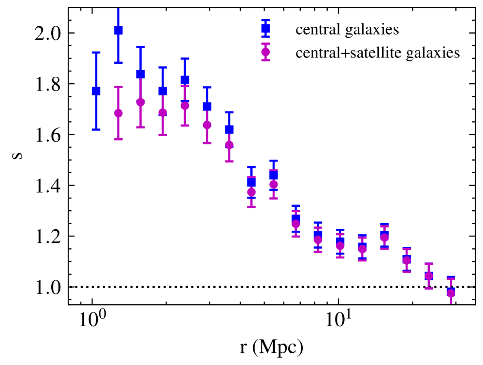
Figure 5: The bias separability function with and without satellite galaxies, measured from a galaxy catalogue based on Abacus Summit Huge simulations.

5 Summary and Conclusion

In this work, we investigated a commonly used simplification in the halo model—the assumption of halo bias separability, where the halo bias of two halo populations of different masses is expressed as a separable function of their masses (i.e. $b^{2}_{\rm hh}(M_{1},M_{2})=b(M_{1})\,b(M_{2})$). Unlike previous studies (e.g. Mead & Verde 2021), we explicitly disentangled this assumption from the scale dependence of halo bias. In particular, we examined the separability assumption using the Abacus dark matter $N$-body simulations covering the redshift range $0\leq z\leq 3$, and bright galaxy samples from the HSC-SSP Wide survey with a median redshift of $\sim 3.6$.

We first defined the halo bias separability function, $s(M_{1},M_{2},r,z)$, via Eq. 9 as the ratio of the cross-correlation function of haloes with masses $M_{1}$ and $M_{2}$ to the square root of the product of their auto-correlation functions. We then measured $s$ from simulations using haloes spanning the mass range $5\times 10^{11}$–$5\times 10^{13}\,\rm M_{\odot}$, typical of those hosting galaxies. The deviation of $s$ from unity directly quantifies the extent to which halo bias is non-separable. Our main findings from the simulations are summarised below:

• Scale dependence: The separability function $s$ deviates from unity on quasi-linear scales ($\sim 1$–$5\,\mathrm{Mpc}$), indicating a breakdown of bias separability at these scales. At larger separations, $s$ approaches unity, where halo bias is seperable.

• Enhancement vs suppression: Across all redshifts, the separability function $s$ typically exceeds unity on quasi-linear scales, indicating an enhanced clustering of haloes of different masses. Notably, a suppression of $s$ is observed at $z\sim 0$ near $1\,\mathrm{Mpc}$.

• Redshift dependence: At $z\sim 0$, $s$ differs from unity by at most $\sim 10\%$, which increases to $\sim 20\%$ at $z\sim 1$. At $z\sim 3$, $s$ reaches a value as high as 2, indicating a strong break-down of the seperability assumption at high redshifts and leading to the enhancement of halo cross-correlations by the same factor.

• Mass dependence: The deviation of $s$ from unity is larger for more massive haloes. It also increases with the mass separation between the halo mass bins used to measure $s$. At $z\sim 3$, the most massive haloes in our simulations show significant departures from unity even at scales of $\sim 15\,\mathrm{Mpc}$.

To test whether the non-separable bias is observable in galaxy clustering, we use galaxy samples from the HSC-SSP wide survey to measure the separability function at a median redshift of $z\sim 3.6$. Since the masses of individual galaxies are not directly available, we divide the galaxy sample into different UV magnitude bins and compute their angular auto- and cross-correlation functions. From these, we derive the separability function $s(\rm m_{\text{uv1}},\rm m_{\text{uv2}},\theta)$ using Eq. 15. To our knowledge, this provides the first observational evidence for the non-separability of galaxy bias at high redshift, revealing the breakdown of a key halo model approximation in the early Universe. Specifically, we find that:

• The measured $s$ deviates significantly from unity on angular scales $\theta\lesssim 1500^{\prime\prime}$. For example, for samples defined by $20<\rm m_{\text{uv1}}\leq 23.75$ and $24.1<\rm m_{\text{uv2}}\leq 24.5$, $s$ reaches a value of 1.8 at $\theta\sim 100^{\prime\prime}$.

• The larger the separation in magnitude between galaxy samples, the greater the deviation of $s$ from unity. This is consistent with the mass-dependence of $s$ observed in simulations.

To compare the observed separability function with simulations, we estimate an effective halo mass for each galaxy sample using large-scale bias measurements, which is then used to compute $s$ from simulations. The measurements from simulations agree remarkably well with those from observations, confirming that high-redshift galaxy bias is non-separable on quasi-linear scales.

To evaluate the effect of satellite galaxies on the measured separability function, we populated haloes from $N$-body simulations with both centrals and satellites using a simple HOD prescription. The HOD parameters are chosen such that the resulting galaxy number density and satellite fraction are in broad agreement with those of the observed HSC-SSP galaxy sample. Using this mock catalog, we measure $s$ with and without the inclusion of satellites. We find that satellites mildly suppress the deviation of $s$ from unity, but the non-separability signal remains significant in both cases. This suggests that the observed non-separability of halo bias is not a result of satellite contamination. Moreover, the fact that the signal is stronger in the absence of satellites supports the robustness of our findings.

Our results demonstrate that the assumption of halo bias separability breaks down on quasi-linear scales, particularly at high redshifts. This deviation is clearly detectable in observed galaxy clustering with current data. The strong agreement between simulations and observations lends robustness to this conclusion. These findings suggest that the separability function $s$ could serve as a powerful observational tool in upcoming surveys to constrain both galaxy formation physics and cosmological parameters. Future work using larger $N$-body simulations and improved analytic models will be crucial to fully exploring its potential.

References

- Abbott et al. (2022) Abbott T. M. C., et al., 2022, Phys. Rev. D, 105, 023520
- Aihara et al. (2018) Aihara H., et al., 2018, PASJ, 70, S8
- Aihara et al. (2019) Aihara H., et al., 2019, Publications of the Astronomical Society of Japan, 71, 114
- Aihara et al. (2022) Aihara H., et al., 2022, PASJ, 74, 247
- Alam et al. (2017) Alam S., et al., 2017, MNRAS, 470, 2617
- Barkana (2007) Barkana R., 2007, Mon. Not. Roy. Astron. Soc., 376, 1784
- Berlind & Weinberg (2002) Berlind A. A., Weinberg D. H., 2002, ApJ, 575, 587
- Berti et al. (2023) Berti A. M., Dawson K. S., Dominguez W., 2023, ApJ, 954, 131
- Bhowmick et al. (2018) Bhowmick A. K., Di Matteo T., Feng Y., Lanusse F., 2018, MNRAS, 474, 5393
- Bosch et al. (2004) Bosch F. C., Tormen G., Giocoli C., 2004, arXiv preprint astro-ph/0409201
- Bosch et al. (2018) Bosch J., et al., 2018, PASJ, 70, S5
- Bullock et al. (2002) Bullock J. S., Wechsler R. H., Somerville R. S., 2002, MNRAS, 329, 246
- Chaurasiya et al. (2024) Chaurasiya N., More S., Ishikawa S., Masaki S., Kashino D., Okumura T., 2024, MNRAS, 527, 5265
- Conroy et al. (2006) Conroy C., Wechsler R. H., Kravtsov A. V., 2006, ApJ, 647, 201
- Cooray & Sheth (2002) Cooray A., Sheth R., 2002, Phys. Rep., 372, 1
- Coupon et al. (2018) Coupon J., Czakon N., Bosch J., Komiyama Y., Medezinski E., Miyazaki S., Oguri M., 2018, Publications of the Astronomical Society of Japan, 70, S7
- DESI Collaboration et al. (2016) DESI Collaboration et al., 2016, arXiv e-prints, p. arXiv:1611.00036
- Dalmasso et al. (2024) Dalmasso N., Leethochawalit N., Trenti M., Boyett K., 2024, Monthly Notices of the Royal Astronomical Society, 533, 2391
- Dvornik et al. (2023) Dvornik A., et al., 2023, A&A, 675, A189
- Euclid Collaboration et al. (2020) Euclid Collaboration et al., 2020, A&A, 642, A191
- Gao et al. (2023) Gao H., et al., 2023, ApJ, 954, 207
- Garrison et al. (2021) Garrison L. H., Eisenstein D. J., Ferrer D., Maksimova N. A., Pinto P. A., 2021, Monthly Notices of the Royal Astronomical Society, 508, 575
- Giavalisco (2002) Giavalisco M., 2002, Annual Review of Astronomy and Astrophysics, 40, 579
- Gsponer et al. (2024) Gsponer R., Zhao R., Donald-McCann J., Bacon D., Koyama K., Crittenden R., Simon T., Mueller E.-M., 2024, MNRAS, 530, 3075
- Hadzhiyska et al. (2022) Hadzhiyska B., Eisenstein D., Bose S., Garrison L. H., Maksimova N., 2022, Monthly Notices of the Royal Astronomical Society, 509, 501
- Hahn et al. (2024) Hahn C., et al., 2024, Nature Astronomy, 8, 1457
- Harikane et al. (2018) Harikane Y., et al., 2018, Publications of the Astronomical Society of Japan, 70, S11
- Harikane et al. (2022) Harikane Y., et al., 2022, The Astrophysical Journal Supplement Series, 259, 20
- Hsieh & Yee (2014) Hsieh B., Yee H., 2014, The Astrophysical Journal, 792, 102
- Iliev et al. (2003) Iliev I. T., Scannapieco E., Martel H., Shapiro P. R., 2003, Mon. Not. Roy. Astron. Soc., 341, 81
- Ivanov et al. (2020) Ivanov M. M., Simonović M., Zaldarriaga M., 2020, J. Cosmology Astropart. Phys., 2020, 042
- Jiang & Van Den Bosch (2016) Jiang F., Van Den Bosch F. C., 2016, Monthly Notices of the Royal Astronomical Society, 458, 2848
- Jiménez et al. (2019) Jiménez E., Contreras S., Padilla N., Zehavi I., Baugh C. M., Gonzalez-Perez V., 2019, MNRAS, 490, 3532
- Jose et al. (2013a) Jose C., Subramanian K., Srianand R., Samui S., 2013a, MNRAS, 429, 2333
- Jose et al. (2013b) Jose C., Srianand R., Subramanian K., 2013b, MNRAS, 435, 368
- Jose et al. (2016) Jose C., Lacey C. G., Baugh C. M., 2016, MNRAS, 463, 270
- Jose et al. (2017) Jose C., Baugh C. M., Lacey C. G., Subramanian K., 2017, MNRAS, 469, 4428
- Kaiser (1984) Kaiser N., 1984, ApJ, 284, L9
- Kawanomoto et al. (2018) Kawanomoto S., et al., 2018, Publications of the Astronomical Society of Japan, 70, 66
- Kravtsov et al. (2004) Kravtsov A. V., Berlind A. A., Wechsler R. H., Klypin A. A., Gottlöber S., Allgood B., Primack J. R., 2004, ApJ, 609, 35
- LSST Dark Energy Science Collaboration (2012) LSST Dark Energy Science Collaboration 2012, arXiv e-prints, p. arXiv:1211.0310
- Landy & Szalay (1993) Landy S. D., Szalay A. S., 1993, Astrophysical Journal, Part 1 (ISSN 0004-637X), vol. 412, no. 1, p. 64-71., 412, 64
- Lapi & Danese (2021) Lapi A., Danese L., 2021, ApJ, 911, 11
- Lee et al. (2009) Lee K.-S., Giavalisco M., Conroy C., Wechsler R. H., Ferguson H. C., Somerville R. S., Dickinson M. E., Urry C. M., 2009, ApJ, 695, 368
- Limber (1953) Limber D. N., 1953, ApJ, 117, 134
- Mahony et al. (2022) Mahony C., et al., 2022, MNRAS, 515, 2612
- Maksimova et al. (2021) Maksimova N. A., Garrison L. H., Eisenstein D. J., Hadzhiyska B., Bose S., Satterthwaite T. P., 2021, Monthly Notices of the Royal Astronomical Society, 508, 4017
- Masaki et al. (2013) Masaki S., Hikage C., Takada M., Spergel D. N., Sugiyama N., 2013, MNRAS, 433, 3506
- Mead & Verde (2021) Mead A. J., Verde L., 2021, MNRAS, 503, 3095
- Mo & White (1996) Mo H. J., White S. D. M., 1996, MNRAS, 282, 347
- Mons & Jose (2024) Mons E., Jose C., 2024, arXiv preprint arXiv:2412.12573
- Moretti et al. (2023) Moretti C., Tsedrik M., Carrilho P., Pourtsidou A., 2023, J. Cosmology Astropart. Phys., 2023, 025
- Norberg et al. (2009) Norberg P., Baugh C. M., Gaztanaga E., Croton D. J., 2009, Monthly Notices of the Royal Astronomical Society, 396, 19
- Okumura et al. (2021) Okumura T., Hayashi M., Chiu I. N., Lin Y.-T., Osato K., Hsieh B.-C., Lin S.-C., 2021, PASJ, 73, 1186
- Ono et al. (2018) Ono Y., et al., 2018, Publications of the Astronomical Society of Japan, 70, S10
- Park et al. (2016) Park J., Kim H.-S., Wyithe J. S. B., Lacey C. G., Baugh C. M., Barone-Nugent R. L., Trenti M., Bouwens R. J., 2016, MNRAS, 461, 176
- Peebles (1980) Peebles P. J. E., 1980, The large-scale structure of the universe
- Pei et al. (2024) Pei W., et al., 2024, MNRAS, 529, 4958
- Pellejero Ibáñez et al. (2024) Pellejero Ibáñez M., Angulo R. E., Peacock J. A., 2024, MNRAS, 534, 3595
- Pizzati et al. (2024) Pizzati E., Hennawi J. F., Schaye J., Schaller M., 2024, MNRAS, 528, 4466
- Planck Collaboration et al. (2020a) Planck Collaboration et al., 2020a, A&A, 641, A6
- Planck Collaboration et al. (2020b) Planck Collaboration et al., 2020b, A&A, 641, A6
- Reed et al. (2007) Reed D. S., Bower R., Frenk C. S., Jenkins A., Theuns T., 2007, MNRAS, 374, 2
- Scannapieco & Barkana (2002) Scannapieco E., Barkana R., 2002, Astrophys. J., 571, 585
- Schneider et al. (2012) Schneider A., Smith R. E., Macciò A. V., Moore B., 2012, MNRAS, 424, 684
- Scoccimarro et al. (2001) Scoccimarro R., Sheth R. K., Hui L., Jain B., 2001, ApJ, 546, 20
- Scranton et al. (2002) Scranton R., et al., 2002, The Astrophysical Journal, 579, 48
- Seljak (2000) Seljak U., 2000, MNRAS, 318, 203
- Sheth & Tormen (1999) Sheth R. K., Tormen G., 1999, MNRAS, 308, 119
- Shuntov et al. (2025) Shuntov M., et al., 2025, arXiv e-prints, p. arXiv:2503.14280
- Smith et al. (2003) Smith R. E., et al., 2003, MNRAS, 341, 1311
- Smith et al. (2007) Smith R. E., Scoccimarro R., Sheth R. K., 2007, Phys. Rev. D, 75, 063512
- Smith et al. (2011) Smith R. E., Desjacques V., Marian L., 2011, Phys. Rev. D, 83, 043526
- Steidel et al. (1996) Steidel C. C., Giavalisco M., Pettini M., Dickinson M., Adelberger K. L., 1996, The Astrophysical Journal, 462, L17
- Tanaka et al. (2018) Tanaka M., et al., 2018, Publications of the Astronomical Society of Japan, 70, S9
- Tinker et al. (2005) Tinker J. L., Weinberg D. H., Zheng Z., Zehavi I., 2005, The Astrophysical Journal, 631, 41
- Tinker et al. (2010) Tinker J. L., Robertson B. E., Kravtsov A. V., Klypin A., Warren M. S., Yepes G., Gottlöber S., 2010, ApJ, 724, 878
- Tinker et al. (2012) Tinker J. L., et al., 2012, ApJ, 745, 16
- Toshikawa et al. (2018) Toshikawa J., et al., 2018, Publications of the Astronomical Society of Japan, 70, S12
- Toshikawa et al. (2024) Toshikawa J., et al., 2024, MNRAS, 527, 6276
- Valogiannis et al. (2024) Valogiannis G., Yuan S., Dvorkin C., 2024, Phys. Rev. D, 109, 103503
- Van Den Bosch et al. (2007) Van Den Bosch F. C., et al., 2007, Monthly Notices of the Royal Astronomical Society, 376, 841
- White & Rees (1978) White S. D. M., Rees M. J., 1978, MNRAS, 183, 341
- Yang et al. (2003) Yang X., Mo H. J., van den Bosch F. C., 2003, MNRAS, 339, 1057
- Yuan et al. (2024) Yuan S., et al., 2024, MNRAS, 530, 947
- Zehavi et al. (2005) Zehavi I., et al., 2005, The Astrophysical Journal, 630, 1
- Zehavi et al. (2011) Zehavi I., et al., 2011, ApJ, 736, 59
- Zheng et al. (2005) Zheng Z., et al., 2005, ApJ, 633, 791
- van Uitert et al. (2015) van Uitert E., Cacciato M., Hoekstra H., Herbonnet R., 2015, A&A, 579, A26
- van den Bosch et al. (2013) van den Bosch F. C., More S., Cacciato M., Mo H., Yang X., 2013, Monthly Notices of the Royal Astronomical Society, 430, 725