Thermal corrections to dark matter annihilation with real photon emission/absorption

Abstract

The dark matter relic density is being increasingly precisely measured. This relic density is theoretically determined by a Boltzmann equation which computes the dark matter distribution according to the (thermally averaged) cross section for annihilation/production of dark matter within a given model. We present here the complete higher order thermal corrections, calculated using real time thermal field theory, to the cross section for the annihilation of dark matter into Standard Model fermions via charged scalars: $\chi\chi\to f\overline{f}$ and $\chi\chi\to f\overline{f}(\gamma)$. The latter process includes real photon emission into, and absorption from, the heat bath at temperature $T$. We use the Grammer and Yennie technique to separate the soft infra-red divergences, which greatly simplifies the calculation. We show explicitly the cancellation of both soft and collinear divergences between real and virtual contributions at next-to-leading order (NLO) in the thermal field theory and remark on the non-trivial nature of the collinear divergences when the thermal contribution from fermions is considered. We present the leading thermal contributions to order ${\cal{O}}(\alpha T^{2})$ for the case when the dark matter particle is a Majorana or Dirac type fermion. In the former case, both the leading order (LO) and NLO cross sections are helicity suppressed, while neither is suppressed in the Dirac case. It is interesting that the ratio of NLO to LO cross sections is the same for both Majorana and Dirac type dark matter.

Keywords: Thermal field theory, Dark Matter annihilation, real photon emission/absorption

1 Introduction

Thermal corrections to dark matter (DM) annihilation cross sections are of interest due to the precision with which the dark matter relic density has been measured, and given that temperature effects are important in the early Universe. While evidence for DM arises from several astrophysical and cosmological observations [1, 2, 3, 4, 5, 6], its properties are not as yet fully determined since they have not been directly detected; see, for instance, Ref. [7], for a review. However, the existence of DM is considered to be well-established, with a precisely measured relic density (its present abundance in the Universe), $\Omega_{c}h^{2}=0.1200\pm 0.0012$ [1], where $h$ is the reduced Hubble constant, $h=H_{0}/100$, and the subscript $c$ refers to cold dark matter.

There exist many models of DM with differing properties such as such as weakly interacting massive particles, axion-like particles, neutralino dark matter, sterile neutrinos, particles in extra dimensional theories, primordial black holes, etc.; see Refs. [8, 9, 10, 11, 12, 13, 14, 15, 16] for reviews. There are many scenarios like asymmetric dark matter, etc., with freeze-out and freeze-in being two popular mechanisms. In the former case, the DM is considered to be in thermal, chemical and kinetic equilibrium with standard model (SM) particles until its interaction rate falls below the Hubble expansion rate, when the DM freezes out, giving the present relic density. In the freeze-in scenario, the coupling of DM to SM particles is small so that the DM is never in equilibrium with the SM particles; the amount of dark matter in the Universe then keeps on increasing until it freezes-in to the present relic density [19, 20]. In both cases, the theoretical quantity of interest is the collision term, which determines how the relic density evolves using the Boltzmann equation [21]. The collision term is simply related to the cross section for dark matter annihilation/production.

The present-day experimental determination of the dark matter relic density is now so precise that these model-based cross sections need to be calculated to next-to-leading order (NLO); for example, the cross sections in various models have been calculated in Refs. [22, 23, 24, 25, 26, 27, 28]. Additionally, thermal corrections to these cross sections (or decay rates) can become important in the early Universe; see Refs. [29, 30, 31, 32, 33, 34, 35], in Quark Gluon Plasma [36]. Some of the processes have also been resummed [37, 38, 39]. Other work [40] has also discussed in detail the limitations of the Boltzmann equation. In particular, Beneke et al. [33] computed the thermal NLO corrections to the dark matter annihilation cross section in a generic DM model where Majorana dark matter particles interact with SM fermions through charged scalars where they showed that the leading $s$-wave (non-relativistic) contribution to the thermal cross section for the dark matter annihilation to SM fermion pairs via scalars, viz., $\chi\chi\to f\overline{f}$, of order ${\cal O}(\alpha T^{2})$, vanishes in the massless fermion limit, where $T$ is the temperature of the heat bath in which the interaction occurs.

In our earlier work [41], the higher order $({\cal{O}}(\alpha)$) finite thermal contribution at order ${\cal O}(T^{2})$ was independently calculated for virtual corrections for the same process. It was shown that the contribution was suppressed due to helicity suppression, the same as with the leading order (LO) cross section. In this paper, we calculate the ${\cal{O}}(\alpha)$ thermal cross section for the process, $\chi\chi\to f\overline{f}(\gamma)$, that is, the real photon thermal corrections to the annihilation cross section. Here the notation $(\gamma)$ indicates that the real photon may be both emitted into, and absorbed by, the heat bath. Although, in principle, there is now a three-body final state with the possibility to lift the helicity suppression, in contrast to the LO and the virtual NLO thermal corrections, we find that this process is also helicity suppressed. In contrast, annihilation processes involving Dirac (not Majorana) dark matter particles remain helicity un-suppressed [42] at both the LO and NLO and can significantly alter the collision term in the Boltzmann equation and hence alter the dark matter relic density calculations.

In the earlier paper [41], we had directly calculated the finite part of the thermal virtual cross section using the technique of Grammer and Yennie (GY) [43], which collects the infra-red (IR) finite terms into the so-called $G$-photon contribution, while isolating the IR divergences into the so-called $K$-photon terms. This technique was used [44, 45] to prove for the first time, the all-orders cancellation of the IR divergences between the virtual and real contributions, order by order, to all orders in perturbation theory. In this paper, we have calculated the complete real thermal contribution to the dark matter annihilation process; hence we also demonstrate here explicitly the cancellation at NLO of IR divergences between the real and virtual contributions. However, while doing so, we found that the GY technique only separates the soft IR divergences, not the collinear ones. We show here explicitly the cancellation of the collinear divergences between the real and virtual contributions, diagram by diagram, at NLO. The structure of these collinear divergences turns out to be non-trivial and interesting.

In the next Section, we review in brief the generic dark matter model that was used in our earlier work [41] for calculating the NLO thermal contribution to the virtual annihilation cross section. For completeness, we also list the LO and virtual NLO cross sections that were obtained there. Since the details of the $K$ and $G$ photon separation become important in the handling of the IR divergences, we present the key elements of the Grammer and Yennie technique as applicable to thermal field theory in Section 3 for later use. (Appendix A contains some relevant details and Feynman rules for calculations in the real-time formulation of thermal field theory.)

In Section 4 we present the results for the real photon thermal contribution to the dark matter annihilation cross section $\chi\chi\to f\overline{f}(\gamma)$ where the $(\gamma)$ indicates that the photon may be emitted into, or absorbed from, the heat bath at temperature $T$. We use the FeynCalc 10.0.0 [46, 47] software with Mathematica 13.1 [48] for the calculations. We present explicitly here, the cancellation of the soft IR and collinear divergences between the real and virtual contributions. Since the virtual contributions are necessary for demonstrating this cancellation, we present some highlights of this calculation, including a discussion of self energy diagrams, in Appendix B for completeness. We present our conclusions with discussions in Section 5.

2 The model, and the virtual NLO thermal corrections, in brief

We briefly review earlier work [41] where the virtual NLO thermal contribution to the dark matter annihilation cross section $\chi\chi\to f\overline{f}$ was calculated using a generic Lagrangian of the form [49, 33]

$${\cal{L}} =-\frac{1}{4}F_{\mu\nu}F^{\mu\nu}+\overline{{f}}\left(i\not{D}-m_{f}\right){{f}}+\frac{1}{2}\overline{\chi}\left(i\not{\partial}-m_{\chi}\right)\chi$$

$$\qquad+\left(D^{\mu}\phi\right)^{\dagger}\left(D_{\mu}\phi\right)-m_{\phi}^{2}\phi^{\dagger}\phi+\left(\lambda\overline{\chi}P_{L}{{f}}^{-}\phi^{+}+{\rm h.c.}\right)~.$$ (1)

Here the dark matter candidate is an $SU(2)\times U(1)$ singlet Majorana fermion $\chi$ which interacts with SM doublet fermions, $f=(f^{0},f^{-})^{T}$, via scalar partners $\phi=(\phi^{+},\phi^{0})^{T}$ through a Yukawa interaction. The calculations are performed after electro-weak symmetry breaking, so that the $W$ and $Z$ are heavy and their contributions to the higher order corrections can be safely ignored.

The NLO thermal corrections to the annihilation of dark matter via $\chi\chi\to f\overline{f}$ in this model were first studied in Ref. [33] where the cancellation of the infra-red divergences was explicitly demonstrated and the finite remainder calculated to leading order in the temperature, ${\cal O}(T^{2})$. This was then extended in Refs. [44, 45] to a proof of the cancellation of infra-red divergences to all orders in such thermal field theories, using a generalised Grammer and Yennie (GY) technique although the finite remainder was not calculated. The advantage of the GY approach, details of which we present in the next section, is the automatic cancellation of the soft infra-red (IR) divergences so that we can directly compute the finite remainder. This approach was used to calculate the explicitly IR finite remainder in the NLO thermal virtual correction to the dark matter annihilation process, $\chi\chi\to f\overline{f}$, in our earlier work [41].

The LO annihilation contribution is shown in Fig. 1; note that since the dark matter particle is assumed to be a Majorana fermion, both $t$ and $u$ channel diagrams contribute.

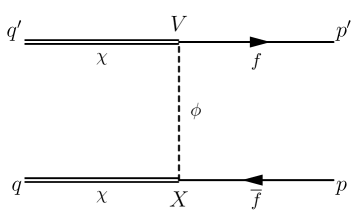
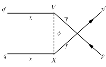
Figure 1: The $t$-channel and $u$-channel dark matter annihilation processes at leading order (LO).

We work in the centre-of-momentum frame where the dark matter particles with momenta $q^{\prime}$ and $q$ collide back-to-back. In the leading order, $P$ and $Q$ are the magnitude of the three-momenta of the fermion (or anti-fermion) and dark matter particles respectively, $s$ is the usual Mandelstam variable, $s=4H^{2}$, $H^{2}=Q^{2}+m_{\chi}^{2}=P^{2}+m_{f}^{2}$, and $m_{i},i=\phi,f,\chi$, are the masses of the scalar, fermion, and dark matter particles respectively.

We perform the calculation in the limit in which the scalar is much heavier than the other particles, viz., $m_{\phi}^{2}\gg m_{\chi}^{2}\gtrsim m_{f}^{2}$. In this limit, the momentum of the scalar, (which is $l\equiv q-p$ in the $t$-channel and $l^{\prime}\equiv q^{\prime}-p$ in the $u$ channel) is such that $l^{2}\sim l^{\prime 2}\ll m_{\phi}^{2}$ (where we have implicitly assumed that $\sqrt{s}\ll m_{\phi}$) so that the scalar propagator can be approximated by $iD_{l_{\phi}}=i/(l^{2}-m_{\phi}^{2})\to-i/m_{\phi}^{2}$; then the LO cross section within this approximation can be expressed as [41]

$$\sigma_{LO}^{\rm Heavy~Scalar} =\frac{1}{32\pi s}\frac{P}{Q}\int\!{\rm d}\!\cos\theta~\left|\rule{0.0pt}{12.0pt}{\cal{M}}_{LO}^{t}-{\cal{M}}_{LO}^{u}\right|^{2}~,$$

$$=\frac{1}{12\pi s}\frac{P}{Q}\frac{\lambda^{4}}{m_{\phi}^{4}}\left[8H^{2}(H^{2}-m_{\chi}^{2})+m_{f}^{2}(5m_{\chi}^{2}-2H^{2})\right]~,$$ (2)

where ${\cal{M}}_{LO}^{t}$ and ${\cal{M}}_{LO}^{u}$ are the matrix elements corresponding to the LO $t$-channel and $u$-channel diagrams shown in Fig. 1. The first term in the square brackets is proportional to $H^{2}-m_{\chi}^{2}\equiv Q^{2}$ and so vanishes in the non-relativistic limit; the second is proportional to $m_{f}^{2}$ and is therefore helicity suppressed because of the nature of the coupling (see Eq. 1). In contrast, the purely $t$-channel contribution (relevant for a Dirac-type dark matter particle) is not helicity suppressed; we have

$$\sigma_{LO}^{\rm Dirac,heavy~scalar} =\frac{1}{12\pi s}\frac{P}{Q}\frac{\lambda^{4}}{m_{\phi}^{4}}\left[H^{2}(4H^{2}-m_{\chi}^{2})-m_{f}^{2}(H^{2}-m_{\chi}^{2})\right]~.$$ (3)

Writing $Q\approx m_{\chi}v$, and replacing the CM velocity $v$ by the relative velocity between the two dark matter particles, $v_{rel}=2v$, the Majorana LO cross section can be written as

$$\sigma_{LO}v_{rel} \overset{Heavy~Scalar}{\xrightarrow{~~~~~~~~~~~~}}\frac{\lambda^{4}}{48\pi}\left[\frac{1}{m_{\phi}^{4}}\right]\left[6m_{f}^{2}+v^{2}\left(16m_{\chi}^{2}-7m_{f}^{2}\right)\right]\left[1-\frac{m_{f}^{2}}{2m_{\chi}^{2}}\right]~,$$ (4)

where we have retained terms upto order ${\cal{O}}(v^{2})$.

The thermal average of this quantity is the collision term of interest in the Boltzmann equation to compute the dark matter relic density: to leading order we have

$$\langle\sigma_{LO}v_{rel}\rangle_{T} \overset{Heavy~Scalar}{\xrightarrow{~~~~~~~~~~~~}}\frac{\lambda^{4}}{48\pi}\left[\frac{1}{m_{\phi}^{4}}\right]\left[6m_{f}^{2}+\frac{3T}{2m_{\chi}}\left(16m_{\chi}^{2}-7m_{f}^{2}\right)\right]\left[1-\frac{m_{f}^{2}}{2m_{\chi}^{2}}\right]~,$$ (5)

where we have used the non-relativistic Maxwell-Boltzmann distribution function [21] for the dark matter particles so that $\langle v^{2}\rangle_{T}=3T/(2m_{\chi})$.

2.1 The thermal NLO virtual contribution to the annihilation cross section

The NLO virtual corrections arise from the combined contributions of ${\cal{M}}_{LO}^{t,u}$, the LO diagrams in Fig. 1 and the contributions ${\cal{M}}_{NLO}^{1\hbox{--}5}$ from the set of NLO diagrams labelled 1–5 in Fig. 2 with virtual photon of momentum $k$.

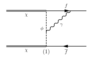
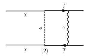
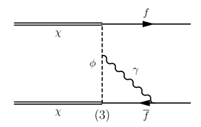
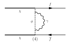
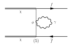
Figure 2: The $t$-channel virtual photon corrections to the dark matter annihilation process at NLO. Diagrams are labelled from 1–5. Analogous contributions from the $u$-channel diagrams exist.

We use the Feynman rules for thermal field theory given in Appendix A. In the real-time formulation of thermal field theory that we use here, there is a field-doubling with type-1 and type-2 thermal fields, so that the propagator is a $2\times 2$ matrix. The propagator can be expressed as a sum of $T$-independent and $T$-dependent parts; the $T$-dependent part allows for a transition between the two types of fields. In particular, it gives rise to the corresponding thermal contribution in the case of virtual photon NLO corrections. All external particles are of type-1 alone; see Appendix A for more details.

Note that the so-called leading order diagrams in Fig. 1 also contribute at the NLO as ${\cal{M}}_{NLO}^{6,7}$ via self-energy diagrams labelled 6–7 in Fig. 3; see Appendix B for more details.

We can write the NLO virtual contribution as the coefficient of the ${\cal{O}}(\alpha)$ term in

$$\sigma_{NLO}^{Virtual} \propto \int\left|{\cal{M}}_{LO}^{t}-{\cal{M}}_{LO}^{u}+{\cal{M}}_{NLO}^{1\hbox{--}7,t}-{\cal{M}}_{NLO}^{1\hbox{--}7,u}\right|_{\alpha}^{2}~,$$ (6)

where we have suppressed the phase space and other factors in the interest of clarity, and the subscript $\alpha$ indicates that we are considering only the NLO contribution. Each of the higher order $t$-channel matrix elements in Eq. 6 gets contributions from the $t$-channel diagrams shown in Figs. 2 and 3 (and similarly, their $u$-channel counterparts).

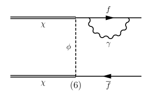
Figure 3: The $t$-channel fermion (L) and anti-fermion (R) virtual photon self-energy corrections to the dark matter annihilation process at next to leading order (NLO). Analogous contributions from the $u$-channel diagrams exist. See Appendix B for details.

Since the dark matter particle is assumed to be Majorana, both the $t$-channel diagrams shown here and their crossed $u$-channel counterparts, along with the $tu$ cross contributions also exist; in contrast, only the $t$-channel diagrams contribute when the dark matter particle is a Dirac fermion. While we have calculated both the ${\cal{O}}(T^{2})$ and ${\cal{O}}(T^{4})$ NLO corrections both in the relativistic case and in the non-relativistic limit using the Grammer and Yennie approach, we present here the dominant ${\cal{O}}(T^{2})$ results. There are three different thermal contributions possible: one where the the photon propagator contributes through its thermal part, and the others where the fermion or anti-fermion propagator contribute through their thermal parts. In what follows, we shall refer to these as the virtual thermal photon, thermal fermion and thermal anti-fermion contributions respectively. Note that the case where both the photon and fermion/anti-fermion are thermal is kinematically disallowed (see Ref. [41] for details).

The thermal virtual contribution at NLO is given by the sum of the thermal photon, thermal fermion, and thermal anti-fermion contributions. Since the thermal contribution is already at order ${\cal{O}}(T^{2})$, we compute only the $s$-wave terms since the $p$-wave ones contribute one more power of temperature to the collision term; see Eq. 5; hence, the $s$-wave terms have the most significant contribution at freeze-out when $m_{\chi}/T\sim 20$.

It is clear that Diagrams 2, 6, and 7 from Figs. 2 and 3 contribute at order ${\cal{O}}(1/m_{\phi}^{4})$ in the scalar mass while Diagrams 1, 3, and 5 contribute at order ${\cal{O}}(1/m_{\phi}^{6})$ while Diagram 4 is highly suppressed, at order ${\cal{O}}(1/m_{\phi}^{8})$. In the centre-of-momentum frame, with energy-momentum of the dark matter particles given by $q^{\prime\mu},q^{\mu}=(H,0,0,\pm Q)$ and that of the fermions given by $p^{\prime\mu},p^{\mu}=(H,\pm P\sin\theta,0,\pm P\cos\theta)$, so that the Mandelstam variable $s=4H^{2}$, we obtain:

$$\sigma_{NLO}^{Virtual}(s\hbox{-wave}) =\frac{\alpha\lambda^{4}}{128}~\frac{m_{f}^{2}\,T^{2}}{\sqrt{s}Q}\left[-\frac{8}{m_{\phi}^{4}}+\frac{32m_{\chi}^{2}}{3m_{\phi}^{6}}+\frac{128m_{\chi}^{4}}{3m_{\phi}^{8}}\right]+{\cal{O}}(v^{2})~,$$

$$=\frac{\alpha\lambda^{4}}{128}~\frac{m_{f}^{2}\,T^{2}}{m_{\chi}^{2}v_{rel}}\left[-\frac{8}{m_{\phi}^{4}}+\frac{32m_{\chi}^{2}}{3m_{\phi}^{6}}+\frac{128m_{\chi}^{4}}{3m_{\phi}^{8}}\right]+{\cal{O}}(v^{2})~.$$ (7)

The NLO virtual thermal cross section was computed in our earlier work [41]; the leading NLO contribution was also calculated earlier by Ref. [33] who explicitly showed the cancellation of soft and collinear divergences at NLO. The NLO thermal cross section was found to vanish in Ref. [33] in the massless limit; this was subsequently explained by them using the Operator Product Expansion approach in Ref. [50] where the cross section for annihilation of Dirac-type dark matter particles was also computed. In our earlier work, we had used the GY technique to directly calculate the IR finite $G$ photon contribution and we had dropped the logarithmic terms that give rise to collinear divergences since they had been shown [33] to cancel. In this paper, since we have now computed the real photon thermal contributions, we will explicitly address the issue of cancellation of collinear divergences and show that the structure of collinear terms is interesting and non-trivial.

Notice the factor $m_{f}^{2}$ in all terms due to helicity suppression of the Majorana dark matter annihilation channel; in contrast, we see below that the Dirac dark matter annihilation cross section is not helicity suppressed:

$$\sigma_{NLO}^{Dirac,Virtual}(s\hbox{-wave}) =\frac{\alpha\lambda^{4}}{128}~\frac{T^{2}}{m_{\chi}^{2}}\left[-\frac{4(2m_{\chi}^{2}+m_{f}^{2})}{m_{\phi}^{4}}+\frac{16m_{\chi}^{2}(2m_{\chi}^{2}-m_{f}^{2})}{3m_{\phi}^{6}}\right.$$

$$\qquad\qquad\left.+\frac{64m_{\chi}^{4}(2m_{\chi}^{2}-3m_{f}^{2})}{3m_{\phi}^{8}}\right]+{\cal{O}}(v^{2})~.$$ (8)

Before we go on to compute the NLO thermal corrections with real photon emission/absorption, we outline the Grammer and Yennie technique for use in the later sections. The informed reader may prefer to skip to Section 4.

3 Infra-red divergences and the Grammer and Yennie technique

We have used the Grammer and Yennie (GY) technique to calculate the IR finite part of the cross section for both the virtual and real photon cases. We now summarise this approach which helps simplify the separation of the soft infra-red (IR) divergences. The GY technique [43, 51] was used to factorise the infra-red (IR) divergences in a zero temperature quantum field theory. There are additional linear IR divergences due to photons in a thermal field theory. Hence the demonstration of cancellation of IR divergences includes demonstrating the cancellation of both the linear and (sub-leading) logarithmic divergences in the thermal theory. Note that there are no additional ultra-violet (UV) divergences because the number operator in both the thermal propagators and phase space acts as a damping factor. The GY technique was extended to the case of thermal field theory, first for fermionic thermal QED [52], and later for charged thermal scalars and fermions interacting with dark matter particles with thermal QED corrections [44, 45], where it was shown that the infra-red divergences cancel between virtual and real photon insertions, order by order, to all orders. The technique uses the fact that only the photon contributions are IR divergent, while fermion insertions do not lead to additional IR divergences. The IR divergences cancel between virtual and real photon insertions as discussed below.

Consider first the insertion of a virtual photon with momentum $k$ into a lower order graph. The procedure starts with writing the virtual photon propagator as the sum of two parts, the so-called $K$ and $G$ photons:

$$-ig^{\mu{\nu}} \to{-i}\left\{\left[g^{\mu\nu}-b_{k}(p_{f},p_{i})\,k^{\mu}k^{\nu}\right]+\left[b_{k}(p_{f},p_{i})k^{\mu}k^{\nu}\right]\right\}~,$$

$$\equiv{-i}\left\{\left[G_{k}^{\mu\nu}\right]+\left[K_{k}^{\mu\nu}\right]\right\}~.$$ (9)

The IR divergence is completely contained in the $K$ photon contribution while the $G$ photon contribution is IR finite. The notation $p_{f}$ and $p_{i}$ is used to separate the final and initial “legs” (where the photon is inserted at vertices $\mu,\nu$) which are defined as being to the right or left of the special vertex $V$ (see Fig. 1) at which the momentum $q^{\prime}$ is guaranteed to be hard (not soft). Hence, for the $t$-channel diagram in Fig. 1, the fermion line with $p_{f}=p^{\prime}$ is defined as the final “leg” while the anti-fermion and scalar lines together form the initial leg with $p_{i}=p$; for the $u$-channel diagrams, the scalar forms a part of the $p^{\prime}$ leg instead. Then the factor $b_{k}$ is given by

$$b_{k}(p_{f},p_{i})=\frac{1}{2}\left[\frac{(2p_{f}-k)\cdot(2p_{i}-k)}{((p_{f}-k)^{2}-m^{2})((p_{i}-k)^{2}-m^{2})}+(k\leftrightarrow-k)\right]~,$$ (10)

is defined symmetrically in $k\to-k$ for the thermal case (in contrast to the original definition in Ref. [43]), and is a function of $k$ as well as the momenta, $p_{f}$, $p_{i}$. It can then be shown that the $K$ photon insertions contain the IR divergent pieces while the $G$ photon contribution is IR finite. The proof is long; but the key point is that the insertion of an additional virtual $K$ thermal photon with momentum $k$ in all possible ways into a lower ($n^{\rm th}$) order graph results in the following factorisation of the consequent $(n+1)^{\rm th}$ order matrix element in terms of the lower $n^{\rm th}$ order matrix element:

$${\cal{M}}_{n+1}^{K{\rm photon,tot}} =\left[\frac{ie^{2}}{2}\int\frac{{\rm d}^{4}k}{(2\pi)^{4}}\,D^{11}(k)\,\left[b_{k}(p^{\prime},p^{\prime})-2b_{k}(p^{\prime},p)+b_{k}(p,p)\right]\rule{0.0pt}{16.0pt}\right]{\cal{M}}_{n}~,$$

$$\equiv\left[B\right]{\cal{M}}_{n}~,$$ (11)

where $D^{11}(k)$ is the $(11)$ element of the photon propagator (excluding the tensor $g^{\mu\nu}$ term); see Eqs. A.1, A.2, and its $T$-dependent part contains the number operator, $n_{B}(|k^{0}|)$. Notice that the prefactor $B$ contains the entire $k$ dependence and is IR divergent.

While the factorisation of the IR divergent part occurs in the matrix element for virtual photon insertions, it occurs in the square of the matrix elements for the real photon case. Note that both emission and absorption of real photons into/from the heat bath are possible in the thermal case; in fact, this is essential in order to show the IR divergence cancellation between virtual and real photon contributions. When a real photon with momentum $k$ is inserted into a lower order diagram at a vertex $\mu$, the polarisation sum in the squared matrix element can be re-written in terms of the $\widetilde{K}$ and $\widetilde{G}$ contributions:

$$\begin{array}[]{rcl}\displaystyle\sum\limits_{\rm pol}\epsilon^{\mu*}(k)\,\epsilon^{\nu}(k)=\displaystyle-g^{\mu\nu}&=&\displaystyle-\left\{\left[g^{\mu\nu}-\tilde{b}_{k}(p_{f},p_{i})k^{\mu}k^{\nu}\right]+\left[\tilde{b}_{k}(p_{f},p_{i})k^{\mu}k^{\nu}\right]\right\}~,\\[8.61108pt] &\equiv&\displaystyle-\left\{\left[\widetilde{G}_{k}^{\mu\nu}\right]+\left[\widetilde{K}_{k}^{\mu\nu}\right]\right\}~,\end{array}$$ (12)

with $\tilde{b}_{k}(p_{f},p_{i})=b_{k}(p_{f},p_{i})|_{k^{2}=0}$ for real photons. Again, $p_{i}$ ($p_{f}$) is the momentum $p^{\prime}$ or $p$ depending on whether the real photon insertion was on the $p^{\prime}$ or $p$ leg in the $n^{\rm th}$ order matrix element ${\cal M}_{n+1}$ (or its conjugate ${\cal M}_{n+1}^{\dagger}$). As in the case for virtual $K$ photon insertion, the insertion of a $\widetilde{K}$ real photon into an $n^{\rm th}$ order graph leads to a cross section that is proportional to the lower order one by an overall factor analogous to that in Eq. 11 for virtual photon insertion:

$$\left|{\cal{M}}_{n+1}^{\widetilde{K}\gamma,{\rm tot}}\right|^{2} \propto-e^{2}\left[\tilde{b}_{k}(p,p)-2\tilde{b}_{k}(p^{\prime},p)+\tilde{b}_{k}(p^{\prime},p^{\prime})\right]\left|{\cal{M}}_{n}^{{\rm tot}}\right|^{2}~.$$

Since we are dealing with real photon insertions, recall that the phase space factor also contains $k$ dependence:

$$\int{\rm d}P_{k}\equiv\int\frac{{\rm d}^{4}k}{(2\pi)^{4}}2\pi\delta(k^{2})\left[\theta(k^{0})(1+n_{B}(|k^{0}|))+\theta(-k^{0})n_{B}(|k^{0}|)\right]~,$$ (13)

where the two terms account for both the probability of emission into a heat bath at temperature $T$ (proportional to $(n_{B}(|k^{0}|)+1)$) and absorption from the heat bath (proportional to $n_{B}(|k^{0}|)$). Then the total $k$-dependent part that factorises out of the expression can be written as [44, 45],

$$\widetilde{B}(x)=-e^{2}\int{\rm d}P_{k}\left[\tilde{b}_{k}(p,p)-2\tilde{b}_{k}(p^{\prime},p)+\tilde{b}_{k}(p^{\prime},p^{\prime})\right]\exp\left[{\pm i\,k\cdot x}\right]~,$$ (14)

where the $\pm$ sign depends on whether the photon with momentum $k$ is emitted/absorbed. After some simplification, and including the finite contributions from the $G$ and $\widetilde{G}$ insertions, the total cross section can be expressed as

$$\sigma^{\rm tot} =\int{\rm d}^{4}x\,e^{-i(q^{\prime}+q-p^{\prime}-p)\cdot x}\,{\rm d}P_{p^{\prime}}{\rm d}P_{p}\exp\left[B+B^{*}+\widetilde{B}\right]\,\sigma^{\rm finite}(x)~.$$ (15)

Here $\sigma^{\rm finite}$ contains the finite $G$ and $\widetilde{G}$ photon contributions from the virtual and real thermal photons respectively, as well as the (finite) thermal fermion contributions. In the limit $k\to 0$, the exponential IR divergent parts of both the virtual and real photon contributions can be seen to cancel:

$$(B+B^{*})+\widetilde{B} \stackrel{{\scriptstyle k\to 0}}{{\longrightarrow}}~0+{\cal O}(k^{2})~.$$ (16)

Hence the total cross section is IR finite to all orders, with the IR divergent part of the real photon cross section cancelling against the corresponding IR divergent part of the virtual contribution. We will use this approach to compute the real thermal corrections to dark matter annihilation processes. In the next section, we will therefore compute the finite remainder at ${\cal{O}}(\alpha)$ arising from the finite combination, $[(B+B^{*})+\widetilde{B}]$, which we shall label, for convenience, as $(K+\widetilde{K})$, and the finite contribution, $\widetilde{G}$. With this summary explanation of the GY technique as well as the discussion on the virtual photon NLO thermal corrections in the previous section, we now go on to the main results of this paper.

4 The real photon thermal contribution to the dark matter annihilation cross section

The thermal contributions to $\chi\chi\to f\overline{f}(\gamma)$ arise from insertions of real photons into the set of LO diagrams shown in Fig. 1, which can be both emitted into or absorbed from the heat bath at temperature $T$. The relevant $t$-channel diagrams $R1,R2,R3$ are shown in Fig. 4 while the corresponding $u$-channel diagrams $R4,R5,R6$ are obtained by crossing these diagrams.

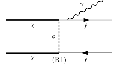
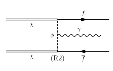
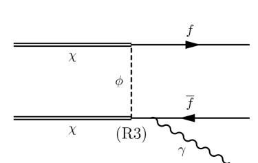
Figure 4: The $t$-channel real photon emission diagrams contributing to the dark matter annihilation process at next to leading order (NLO). Diagrams are labelled from $R1$–$R3$. Similar terms contribute when the photon is instead absorbed from the heat bath. Analogous contributions from the $u$-channel diagrams also exist.

In contrast to the virtual photon case where the thermal ${\cal{O}}(\alpha)$ contribution arose from the product of the NLO (virtual) matrix elements of the diagrams in Fig. 2 with the LO matrix elements in Fig. 1, the ${\cal{O}}(\alpha)$ thermal contribution in the real case arises from the square of the matrix elements corresponding to the diagrams in Fig. 4.

A quick look at the diagrams in Fig. 4 is sufficient to realise that all particles contribute through their type-1 thermal fields at every vertex. As defined in Appendix A, propagators (for photons, scalars and fermions) are given as the sum of a temperature-independent part and a temperature dependent part, the latter of which is on-shell and weighted by the appropriate (Fermi Dirac or Bose Einstein) distribution function. It can be seen that neither of the fermion or anti-fermion propagators can contribute through their thermal parts since three particles at a vertex are kinematically forbidden to be all on-shell. Hence, all thermal contributions to the dark matter annihilation process with real photon emission/absorption arise from the corresponding phase space elements. For a particle with momentum $p$ and mass $m_{p}$, the phase space factor is given by

$$dP_{p}=\int\frac{{\rm d}^{4}p}{(2\pi)^{4}}\left(2\pi\delta(p^{2}-m_{p}^{2})\right)\left[\theta(p^{0})\pm n(|p^{0}|)\right]~.$$ (17)

Here the second term is the thermal contribution, proportional to $n\equiv n_{B}\,(n_{F})$, the Bose (Fermi) distribution function, for bosons and fermions respectively, with the $+\,(-)$ sign corresponding to bosons (fermions). In the calculation that follows, only one of the particles (photon, fermion, anti-fermion) at a time is taken to contribute via its thermal part, since the cross section is otherwise suppressed by products of distribution functions. We therefore have three contributions from each diagram in Fig. 4 (and its $u$-channel counterparts): when each of the real photon, fermion, or anti-fermion contributes via the thermal part of its phase space. We shall refer to them as the real thermal photon, thermal fermion, and thermal anti-fermion contributions respectively.

We apply the Grammer and Yennie technique [43] as explained in Section 3. Hence each of the thermal photon contributions can be separated into $\widetilde{K}$ and $\widetilde{G}$ parts by applying the GY technique. However, it turns out that while the GY technique isolates the soft IR divergence into the $\widetilde{K}$ (and $K$) photon contribution, it fails to separate the collinear divergence the same way. Hence, in what follows, we shall first demonstrate the cancellation of the soft IR divergences between the $\widetilde{K}$ and $K$ photon contributions, while suppressing the collinear terms, and deal with the collinear divergences separately, in a different section, Section 4.4, where we show explicitly that these logarithmic terms cancel between real and virtual contributions. It therefore appears that the use of the GY technique is restricted to those processes where the collinear divergences are independently known to factorise and cancel between virtual and real contributions, order by order in the theory. Even so, there is an advantage in using the GY technique since the divergences cancel at the integrand level and simplify the calculation.

4.1 Kinematics of   $\chi\chi\to f\,\overline{f}\,(\gamma)$

We consider the real photon emission/absorption process in the centre of momentum frame where the dark matter particles have common energy-momentum $q^{\prime},q=(H,0,0,\pm Q)$. We use the same kinematics as in the virtual case, except for the fact that physical momentum $k$ is gained or lost in the real photon process, so that the fermion (with momentum $p^{\prime}$) and anti-fermion (with momentum $p$) no longer have the same energy or momentum (magnitude). The real photon cross section is given by the sum of 21 contributions as follows:

$$\sigma_{NLO}^{Real} =\left[\sum_{i=1}^{6}\sigma_{i,i}^{Real}+(-1)^{S_{p}}\sum_{i<j}^{6}\sigma_{i,j}^{Real}\right]~,$$ (18)

where the individual terms are defined in terms of the squares of various matrix elements:

$$\sigma_{i,i}^{Real} =\frac{1}{4\sqrt{s}Q}\int{\rm d}P_{p^{\prime}}{\rm d}P_{p}{\rm d}P_{k}(2\pi)^{4}\delta^{4}(q^{\prime}\!+\!q\!-\!p^{\prime}\!-\!p\!-\!k)\!\left|M_{R_{i}}\right|^{2}~,$$

$$\sigma_{i,j}^{Real} =\frac{1}{4\sqrt{s}Q}\int{\rm d}P_{p^{\prime}}{\rm d}P_{p}{\rm d}P_{k}(2\pi)^{4}\delta^{4}(q^{\prime}\!+\!q\!-\!p^{\prime}\!-\!p\!-\!k)\!\left|M_{R_{i}}M_{R_{j}}^{\dagger}+h.c.\right|^{2}~,$$ (19)

with $-\infty\leq k^{0}\leq\infty$, thus allowing for both emission and absorption of the real photon, and

$$S_{p} =0~;~~i,j\in\{1,2,3\}\hbox{ or }\{4,5,6\}~,$$

$$=1~;~~i\in\{1,2,3\}\hbox{ and }j\in\{4,5,6\}~.$$ (20)

Here the phase space factors $dP_{i}$ are defined in Eq. 17, and the matrix elements correspond to the three $t$-channel diagrams $R1,R2,R3$ as seen in Fig. 4 and $R4,R5,R6$ are their $u$-channel counterparts. Therefore $\sigma_{i,j}$, $i,j\in 1$–3, are from the $t$-channel diagrams, $\sigma_{i,j}$, $i,j\in 4$–6, are from the $u$-channel diagrams, and the remaining from the crossed $tu$-channel diagrams. In addition, each of these have contributions from three distinct sets of terms: when the photon is thermal, when the fermion is thermal, and when the anti-fermion is thermal. That is, we can write

$$\sigma_{i,j}^{Real} =\sigma_{i,j}^{\gamma,Real}+\sigma_{i,j}^{f,Real}+\sigma_{i,j}^{\overline{f},Real}~,$$ (21)

for all values of $(i,j)$, where the contributions correspond to including the thermal part of the phase space in Eq. 19 for the photon, fermion and anti-fermion respectively.

The frame used for the computation is as follows: of the two non-thermal particles, one is integrated out using the energy-momentum conserving delta function shown in Eq. 19. The other one is rotated into the $z$-direction with energy-momentum $(E^{\prime},0,0,P^{\prime})$, while the thermal particle is arbitrarily aligned in the direction $\hat{n}^{\prime}(\Omega^{\prime})$ defined by the angular coordinates $(\theta^{\prime},\phi^{\prime})$. This allows for the simplest kinematics, and yields, for instance, when the photon is thermal with momentum $k^{\mu}=(k^{0},K\hat{n}^{\prime})$, the anti-fermion momentum is integrated out, and the fermion is rotated into the $z$-axis:

$$\sigma_{i,j}^{\gamma,Real} =\frac{1}{32\sqrt{s}Q}\frac{1}{2(2\pi)^{3}}\int_{0}^{\omega_{max}}\hskip-14.22636pt{\rm d}\omega\int_{E^{\prime}_{min}}^{E^{\prime}_{max}}{\rm d}E^{\prime}\int_{-1}^{1}\!\!{\rm d}\!\cos\theta\int_{0}^{2\pi}{\rm d}\phi^{\prime}$$

$$\qquad\qquad\times~n_{B}(\omega)\left[F_{i,j}^{+}(\omega,\omega,\Omega^{\prime})+F_{i,j}^{-}(-\omega,\omega,\Omega^{\prime})\right]~,$$ (22)

where $\omega=|k^{0}|$, the factor $n_{B}(\omega)$ has been taken out of the integrand to show the dependence on the distribution function, and only the $k^{\mu}$ dependence of the integrand, $F^{\pm}_{i,j}(k^{0},K,\Omega^{\prime})$, has been indicated. Here $\theta$ is the angle between the (rotated) $z$-axis and the dark matter momentum direction; while the thermal photon angle $\theta^{\prime}$ is given by

$$\cos\theta^{\prime}=\frac{(s-2\sqrt{s}(E^{\prime}\pm\omega)\pm 2E^{\prime}\omega)}{2P^{\prime}\omega}~.$$ (23)

The $\pm$ signs correspond to the case of emission/absorption of the photon. The limits on $E^{\prime}$ are obtained from constraints on $|\cos\theta^{\prime}|<1$ while $\omega_{max}=(s-m_{f}^{2})/(2\sqrt{s})$.

When the thermal fermion contribution is under consideration, the anti-fermion momentum is integrated out as in the thermal photon case, and the photon is rotated into the $z$-axis, so that $k^{\mu}=(E^{\prime},0,0,E^{\prime})$. In this case, the fermion has momentum $p^{\prime\mu}=(p^{\prime 0},K_{t}\hat{n}^{\prime})$, and we get an expression analogous to Eq. 22 for $\sigma_{i,j}^{f,Real}$, while also accounting for the fact that the distribution function $n_{B}(\omega)$ in Eq. 22 is to be replaced by $(-n_{F}(\omega_{t}))$ as per the phase space definition in Eq. 17; furthermore, the fermion has non-zero mass so that the thermal fermion angle $\theta^{\prime}$ is given by

$$\cos\theta^{\prime}=\frac{(s-2\sqrt{s}(E^{\prime}\pm\omega_{t})\pm 2E^{\prime}\omega_{t})}{2E^{\prime}K_{t}}~,$$ (24)

where the thermal fermion energy and momentum magnitude are represented by $\omega_{t}=|p^{\prime 0}|$, and $K_{t}$ with $\omega_{t}^{2}=K_{t}^{2}+m_{f}^{2}$ to distinguish them from the massless photon contribution. The case for thermal anti-fermion merely exchanges the fermion and anti-fermion momenta and is straightforward.

In all cases, it can be seen from Eq. 22 that high energy contributions are suppressed due to the presence of the appropriate distribution functions,

$$n_{B}(\omega) =\frac{1}{\exp[\beta\omega]-1}~,$$

$$n_{F}(\omega_{t}) =\frac{1}{\exp[\beta\omega_{t}]+1}~.$$ (25)

Hence, the upper limit on $\omega$ ($\omega_{t}$) can be taken to be infinity so that these integrals can be analytically performed. The leading thermal contribution of order ${\cal{O}}(T^{2})$ then arises from the integrals:

$$\int_{0}^{\infty}\omega\,{\rm d}\omega\,n_{B}(\omega) =\frac{\pi^{2}T^{2}}{6}~,$$

$$\int_{0}^{\infty}\omega_{t}\,{\rm d}\omega_{t}\,n_{F}(\omega_{t}) =\frac{\pi^{2}T^{2}}{12}~,$$ (26)

where we have assumed the massless limit for the thermal fermion integration.

4.2 The matrix elements

The relevant matrix elements for the real photon emission/absorption process $\chi\chi\to f\overline{f}(\gamma)$ corresponding to the diagrams $R1$–$R3$ shown in Fig. 4 are

$$M_{R1} =\frac{ie|\lambda|^{2}}{2k\cdot p^{\prime}~l_{\Phi}}\left[\overline{v}(q,m_{\chi})P_{L}\,v(p,m_{f})\right]\left[\overline{u}(p^{\prime},m_{f})\gamma_{\mu}\left(\not{k}+\not{p}^{\prime}+m_{f}\right)P_{R}\,u(q^{\prime},m_{\chi})\right]\epsilon_{k}^{*\mu}~;$$

$$M_{R2} =\frac{ie|\lambda|^{2}}{lk_{\Phi}~l_{\Phi}}\left(2l-k\right)_{\mu}\left[\overline{v}(q,m_{\chi})P_{L}v(p,m_{f})\right]\left[\overline{u}(p^{\prime},m_{f})P_{R}\,u(q^{\prime},m_{\chi})\right]\epsilon_{k}^{*\mu}~;$$

$$M_{R3} =\frac{ie|\lambda|^{2}}{2k\cdot p~lk_{\Phi}}\left[\overline{v}(q,m_{\chi})P_{L}\left(-\not{k}-\not{p}+m_{f}\right)\gamma_{\mu}\,v(p,m_{f})\right]\left[\overline{u}(p^{\prime},m_{f})P_{R}\,u(q^{\prime},m_{\chi})\right]\epsilon_{k}^{*\mu}~.$$ (27)

Here $P_{R,L}=(1\pm\gamma_{5})/2$, $l_{\Phi}\equiv(l^{2}-m_{\phi}^{2})$ arises from the propagator of the scalar with momentum $l=q-p$. Similarly, $lk_{\Phi}=(l-k)^{2}-m_{\phi}^{2}$. The $u$-channel matrix elements can be obtained by crossing, with momentum $l^{\prime}=q^{\prime}-p$ replacing $l$.

It can be seen from Eq. 27 that the squared matrix elements contain products of the photon polarisation tensor, $\epsilon_{k}^{\mu}$, to which the GY-defined polarisation sum shown in Eq. 12 can be applied in order to separate the $\widetilde{K}$ and $\widetilde{G}$ contributions in the thermal photon case. Since there are known to be no IR divergences [44, 45] in the thermal fermion contributions, the standard polarisation sum,

$$\sum\limits_{\rm pol}\epsilon_{k}^{\mu*}\,\epsilon_{k}^{\nu}=-g^{\mu\nu}~,$$ (28)

is used in this case.

The angular integrals were performed using FeynCalc 10.0.0 [46, 47] software with Mathematica 13.1 [48]. We will first discuss the soft IR and collinear divergences in the next sections, before we consider the finite contribution. The soft IR divergences arise from the $\widetilde{K}$ photon contributions. Since only thermal photons contribute to these terms, we now consider the case where the thermal part of the photon phase space (see Eq. 17) contributes.

4.3 The thermal photon contribution and IR divergences

The soft IR divergences are known to cancel between the real and virtual thermal photon contributions. These are contained in the thermal photon contributions while the thermal fermion contributions are IR finite due to the nature of the Fermi distribution function; see Eq. 25. As shown in Refs. [44, 45], the soft IR divergences can be isolated into the virtual $K$ and real $\widetilde{K}$ photon contributions as defined in Eqs. 9, 12. The sum of these two contributions is finite (this was first shown to NLO in Ref. [33]); we will explicitly show below the cancellation of the soft IR divergences between these two contributions, and also compute the finite remainder. Some details of the virtual NLO thermal correction to $\chi\chi\to f\overline{f}$ are given for convenience in Appendix B; for more details, see our earlier work, Ref. [41].

4.3.1 The $\widetilde{K}$ contribution and soft IR divergences

The soft divergence lies in the $\omega$ integrals of the thermal photon contribution to the real photon cross section which we label $\sigma_{i,j}^{\gamma,Real}$ (see Eq. 22); hence we integrate out the angular variables, leaving only the $\omega$ dependence. The $\widetilde{K}$ part of the thermal real photon cross section can be obtained by taking the $\widetilde{K}$ part of the polarisation sum (see Eq. 12) in the expressions for $\sigma_{i,j}^{\gamma,Real}$. We have

$$\sigma_{i,j}^{\gamma,Real} =\frac{e^{2}\pi|\lambda|^{4}}{32\sqrt{s}Q}\frac{1}{2(2\pi)^{3}}\int{\rm d}\omega~n_{B}(\omega)~Int^{\gamma}_{i,j}~,$$

$$Int^{\gamma}_{i,j} =Int^{\widetilde{K}}_{i,j}+Int^{\widetilde{G}}_{i,j}~,$$ (29)

where $Int^{\widetilde{K}}_{i,j}$ is listed for all $(i,j)$ contributions in Table 1. Here we have retained only terms upto order ${\cal{O}}(\omega,m_{f}^{2})$ since the term linear in $\omega$ will give rise to order ${\cal{O}}(T^{2})$ corrections to the cross section. Hence the terms proportional to $1/\omega$ in Table 1 are linearly divergent in the IR. These are expected to cancel against the corresponding contributions from the virtual NLO terms.

$i,j$	Real $Int^{\widetilde{K}}_{i,j}$ from $Int^{\gamma}_{i,j}$	Virtual $Int_{i,j}^{K_{div}}$	$Int^{\widetilde{K}_{fin}}_{i,j}=Int^{\widetilde{K}}_{i,j}+Int_{i,j}^{K_{div}}$
$1,1$	$-m_{\chi}^{2}(\frac{32m_{\chi}^{2}-8m_{f}^{2}}{\omega m_{\phi}^{4}})-\omega(\frac{32m_{\chi}^{2}-8m_{f}^{2}}{m_{\phi}^{4}})$	$m_{\chi}^{2}(\frac{32m_{\chi}^{2}-8m_{f}^{2}}{\omega m_{\phi}^{4}})$	$-\omega(\frac{32m_{\chi}^{2}-8m_{f}^{2}}{m_{\phi}^{4}})$
$2,2$	$-\omega m_{\chi}^{4}(\frac{128m_{\chi}^{2}+96m_{f}^{2}}{m_{\phi}^{8}})$	–	$-\omega m_{\chi}^{4}(\frac{128m_{\chi}^{2}+96m_{f}^{2}}{m_{\phi}^{8}})$
$3,3$	$-m_{\chi}^{2}(\frac{32m_{\chi}^{2}-8m_{f}^{2}}{\omega m_{\phi}^{4}})-\omega(\frac{32m_{\chi}^{2}-8m_{f}^{2}}{m_{\phi}^{4}})$	$m_{\chi}^{2}(\frac{32m_{\chi}^{2}-8m_{f}^{2}}{\omega m_{\phi}^{4}})$	$-\omega(\frac{32m_{\chi}^{2}-8m_{f}^{2}}{m_{\phi}^{4}})$
$4,4$	$-m_{\chi}^{2}(\frac{32m_{\chi}^{2}-8m_{f}^{2}}{\omega m_{\phi}^{4}})-\omega(\frac{32m_{\chi}^{2}-8m_{f}^{2}}{m_{\phi}^{4}})$	$m_{\chi}^{2}(\frac{32m_{\chi}^{2}-8m_{f}^{2}}{\omega m_{\phi}^{4}})$	$-\omega(\frac{32m_{\chi}^{2}-8m_{f}^{2}}{m_{\phi}^{4}})$
$5,5$	$-\omega m_{\chi}^{4}(\frac{128m_{\chi}^{2}+96m_{f}^{2}}{m_{\phi}^{8}})$	–	$-\omega m_{\chi}^{4}(\frac{128m_{\chi}^{2}+96m_{f}^{2}}{m_{\phi}^{8}})$
$6,6$	$-m_{\chi}^{2}(\frac{32m_{\chi}^{2}-8m_{f}^{2}}{\omega m_{\phi}^{4}})-\omega(\frac{32m_{\chi}^{2}-8m_{f}^{2}}{m_{\phi}^{4}})$	$m_{\chi}^{2}(\frac{32m_{\chi}^{2}-8m_{f}^{2}}{\omega m_{\phi}^{4}})$	$-\omega(\frac{32m_{\chi}^{2}-8m_{f}^{2}}{m_{\phi}^{4}})$
$1,2$	0	0	0
$1,3$	$\omega(\frac{32m_{\chi}^{2}-32m_{f}^{2}}{m_{\phi}^{4}})$	0	$\omega(\frac{32m_{\chi}^{2}-32m_{f}^{2}}{m_{\phi}^{4}})$
$1,4$	$-m_{\chi}^{2}(\frac{64m_{\chi}^{2}-48m_{f}^{2}}{\omega m_{\phi}^{4}})-\omega(\frac{64m_{\chi}^{2}}{m_{\phi}^{4}})$	$m_{\chi}^{2}(\frac{64m_{\chi}^{2}-48m_{f}^{2}}{\omega m_{\phi}^{4}})$	$-\omega(\frac{64m_{\chi}^{2}}{m_{\phi}^{4}})$
$1,5+2,4$	$\omega m_{\chi}^{2}(\frac{256m_{\chi}^{2}-96m_{f}^{2}}{m_{\phi}^{6}})$	–	$\omega m_{\chi}^{2}(\frac{256m_{\chi}^{2}-96m_{f}^{2}}{m_{\phi}^{6}})$
$1,6+3,4$	0	0	0
$2,3$	$\omega m_{\chi}^{2}(\frac{256m_{\chi}^{2}-32m_{f}^{2}}{m_{\phi}^{6}})$	0	$\omega m_{\chi}^{2}(\frac{256m_{\chi}^{2}-32m_{f}^{2}}{m_{\phi}^{6}})$
$2,5$	$\omega m_{\chi}^{4}(\frac{512m_{\chi}^{2}-768m_{f}^{2}}{m_{\phi}^{8}})$	–	$\omega m_{\chi}^{4}(\frac{512m_{\chi}^{2}-768m_{f}^{2}}{m_{\phi}^{8}})$
$2,6+3,5$	$\omega m_{\chi}^{2}(\frac{256m_{\chi}^{2}-96m_{f}^{2}}{m_{\phi}^{6}})$	0	$\omega m_{\chi}^{2}(\frac{256m_{\chi}^{2}-96m_{f}^{2}}{m_{\phi}^{6}})$
$3,6$	$-m_{\chi}^{2}(\frac{64m_{\chi}^{2}-48m_{f}^{2}}{\omega m_{\phi}^{4}})-\omega(\frac{64m_{\chi}^{2}}{m_{\phi}^{4}})$	$m_{\chi}^{2}(\frac{64m_{\chi}^{2}-48m_{f}^{2}}{\omega m_{\phi}^{4}})$	$-\omega(\frac{64m_{\chi}^{2}}{m_{\phi}^{4}})$
$4,5$	$\omega m_{\chi}^{2}(\frac{256m_{\chi}^{2}-32m_{f}^{2}}{m_{\phi}^{6}})$	0	$\omega m_{\chi}^{2}(\frac{256m_{\chi}^{2}-32m_{f}^{2}}{m_{\phi}^{6}})$
$4,6$	$\omega(\frac{32m_{\chi}^{2}-32m_{f}^{2}}{m_{\phi}^{4}})$	0	$\omega(\frac{32m_{\chi}^{2}-32m_{f}^{2}}{m_{\phi}^{4}})$
$5,6$	0	0	0

Table 1: The $\widetilde{K}$ real photon contribution $Int^{\widetilde{K}}_{i,j}$ (see Eq. 29) from various diagrams when the photon is thermal. It can be seen that the IR divergent part of the $\widetilde{K}$ contribution exactly cancels against the divergent part of the corresponding $K$ virtual thermal photon contribution, $Int^{K_{div}}_{i,j}$, leaving a finite remainder, which we label as $Int^{\widetilde{K}_{fin}}_{i,j}$. See text for details.

4.3.2 The real–virtual correspondence

In order to determine the virtual terms corresponding to the real ones, we return to the definition of the real cross section in Eqs. 18 and 19. The correspondence is as follows. Consider, for example, the $\sigma_{1,1}^{Real}$ term which arises from the square of the diagram $R1$ shown in Fig. 4 and can be represented by the cut diagram on the left in Fig. 5. The corresponding virtual contribution is then found by shifting the cut on this diagram such that the photon is virtual as shown on the right side of Fig. 5. We label this contribution as $\sigma_{i,j}^{Virtual}$, $(i,j)=(1,1)$, which is given by (see Eq. 6)

$$\sigma_{1,1}^{Virtual} \propto\int\left[\left({\cal{M}}_{LO}^{t}\right)^{\dagger}{\cal{M}}_{NLO}^{6,t}+h.c.\right]~,$$ (30)

which arises from the fermion self-energy term shown as Diagram 6 in Fig. 3 multiplied by the conjugate of the the LO $t$-channel diagram in Fig. 1. (The $h.c.$ term is obtained by moving the cut to the left of the self energy insertion.)

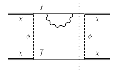
Figure 5: The correspondence between $\sigma_{1,1}^{Real}$ (L) and $\sigma_{1,1}^{Virtual}$ (R) shown diagrammatically through cut diagrams.

Similarly, the virtual counterparts of the $(1,2)$ and $(1,3)$ terms arise from the contributions of the NLO diagrams labelled (1) and (2) repectively in Fig. 2 multiplied by the conjugate of the LO $t$-channel diagram in Fig. 1, etc. The $(1,2)$ correspondence is shown in Fig. 6.

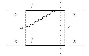
Figure 6: As in Fig. 5 to demonstrate the $(1,2)$ real–virtual correspondence through cut diagrams.

We use the results from our earlier work [41] to obtain the $K$ photon IR divergent parts of the various virtual thermal photon diagrams. These are listed as $Int_{i,j}^{K_{div}}$ in the second column of Table 1, with the same overall factor removed as in the real contribution—see Eq. 29—for ease of comparison.

It can be seen from Table 1 that the divergent parts of $\widetilde{K}$ and $K$ cancel, leaving behind a finite remainder. Contributions such as $(2,2)$ and $(5,5)$ from the square of matrix elements $R2$ and its $u$-channel counterpart $R5$ as well as the $(2,5)$ crossed $tu$-channel contribution must necessarily have no divergent terms as the virtual counterpart does not exist. (The same is true for the virtual diagrams (4), (5) in Fig. 2 which have no real-photon counterparts.) This is indeed seen to hold.

Additionally, we have dropped terms that are collinearly divergent as the fermion mass goes to zero; we will discuss these terms in the next section. For example, it appears as though there is no soft divergent contribution from the $(1,3)$ term, as can be seen from the relevant entry in Table 1; however, there is indeed a soft divergent contribution which is also collinear divergent. We will deal with such terms in the next section. In fact, collinear divergent terms arise in all contributions: the thermal photon, thermal fermion and the thermal anti-fermion terms. All soft IR divergent terms are correctly factored into the $\widetilde{K}$ contributions for the real terms; hence the soft IR divergent terms which are also collinear divergent are contained within the $\widetilde{K}$ contributions, so that the $\widetilde{G}$ contributions are IR finite. However, some of the soft IR finite terms which are collinear divergent are seen to be partially contained in the $\widetilde{K}$ and partially in the $\widetilde{G}$ contributions so that the GY separation for collinear divergences is imperfect. The same is true for the virtual $K$ and $G$ contributions as well. However, overall the collinear divergences do cancel between the real and virtual contributions. We will show the cancellation of these terms in the next section.

4.4 Cancellation of collinear divergences

As mentioned earlier, it turns out that both the $\widetilde{G}$ and $\widetilde{K}$ contributions contain collinear divergences, the sum of which cancel against the sum of the $G$ and $K$ collinear divergent contributions. It is therefore more convenient to discuss the collinear divergences arising from the sum of $\widetilde{G}$ and $\widetilde{K}$ (and from the sum of $K$ and $G$ from the virtual photon contribution). There are three sets of contributing terms, arising from the case when the photon is thermal (with both $\widetilde{G}$ and $\widetilde{K}$ contributing), the fermion is thermal, and the anti-fermion is thermal. Recall that when the photon is thermal, the photon contributes via the thermal part of its propagator in the virtual case, while it contributes via the thermal part of its phase space in the real photon case, and similarly for the other two cases.

In the case of real photons, we have the factor $n_{B}(\omega)$ in the phase space for thermal photons, while we have $(-n_{F}(\omega_{t}))$ for thermal fermions (anti-fermions); see Eq. 17. Hence we compute the collinear contributions in $\sigma^{\gamma,Real}_{i,j}$, the thermal photon contribution to the cross section, as given in Eq. 29, as well as from the thermal fermion contributions, given by

$$\sigma_{i,j}^{f,Real} =-\frac{e^{2}\pi|\lambda|^{4}}{32\sqrt{s}Q}\frac{1}{2(2\pi)^{3}}\int{\rm d}\omega_{t}~n_{F}(\omega_{t})~Int^{f}_{i,j}~,$$ (31)

with an analogous definition for the thermal anti-fermion contribution, $\sigma_{i,j}^{\bar{f},Real}$. These contributions will cancel against the collinear divergent terms from the corresponding virtual contributions. Note that in the case of virtual contributions, the thermal photon, thermal fermion and thermal anti-fermion contributions come from the corresponding thermal parts of their propagators in Diagrams (1)–(7) in Figs. 2 and 3. For more details on the virtual contribution, see Appendix B or Ref. [41].

The relevant real and virtual collinear contributions are listed in Tables 2, 3 and 4, where only the leading $s$-wave results with $v\to 0$ are shown; the exact expressions are available on-line as a Mathematica notebook [53].

It may be noted that the logarithms are not precisely the same in the real and virtual case; they merely match in the collinear (massless) limit. In the case of thermal photons, the structure of the logarithms that contribute in the virtual ($V$) and real ($R$) case is given by

$$L_{V} =\log\left[\frac{H-P}{H+P}\right]\approx\log\left[\frac{m_{f}^{2}}{4H^{2}-m_{f}^{2}}\right]~,$$

$$L_{R} =\frac{1}{2}\left(\log\left[\frac{m_{f}^{2}}{4H^{2}-4H\omega-m_{f}^{2}}\right]+\log\left[\frac{m_{f}^{2}}{4H^{2}+4H\omega-m_{f}^{2}}\right]\right)~,$$

$$L^{\prime}_{R} =\frac{1}{2}\left(\log\left[\frac{m_{f}^{2}}{4H^{2}-4H\omega-m_{f}^{2}}\right]-\log\left[\frac{m_{f}^{2}}{4H^{2}+4H\omega-m_{f}^{2}}\right]\right)~.$$ (32)

Since $\omega$ is strictly less than $(s-m_{f}^{2})/(2\sqrt{s})=H-m_{f}^{2}/(4H)$, we can expand $L_{R}$ and $L^{\prime}_{R}$ as

$$L_{R} =\frac{1}{2}\left(\log\left[\frac{m_{f}^{2}}{4H^{2}-m_{f}^{2}}\left(1+\frac{4H\omega}{4H^{2}-m_{f}^{2}}\right)\right]+\log\left[\frac{m_{f}^{2}}{4H^{2}-m_{f}^{2}}\left(1-\frac{4H\omega}{4H^{2}-m_{f}^{2}}\right)\right]\right),$$

$$\approx\frac{1}{2}\left[2\log\left[\frac{m_{f}^{2}}{4H^{2}-m_{f}^{2}}\right]+{\cal{O}}(\omega)^{2}\right]\equiv L_{V}+{\cal{O}}(\omega)^{2}~,$$

$$L^{\prime}_{R} =\frac{1}{2}\left(\log\left[\frac{m_{f}^{2}}{4H^{2}-m_{f}^{2}}\left(1+\frac{4H\omega}{4H^{2}-m_{f}^{2}}\right)\right]-\log\left[\frac{m_{f}^{2}}{4H^{2}-m_{f}^{2}}\left(1-\frac{4H\omega}{4H^{2}-m_{f}^{2}}\right)\right]\right),$$

$$\approx\frac{1}{2}\left[2\left[\frac{4H\omega}{4H^{2}-m_{f}^{2}}\right]+{\cal{O}}(\omega)^{2}\right]~,$$ (33)

where we have expanded the log terms appropriately. We have retained terms only till order ${\cal{O}}(\omega)$ since higher order terms contribute at order ${\cal{O}}((T/m_{\chi})^{4})$ or higher, and are hence small. It turns out that the coefficient of $L^{\prime}_{R}$, when summed over all $(i,j)$ as shown in Eqs. 18, 19, equals $(0\times m_{\chi}^{2}+{\cal{O}}(m_{f}^{2}))$ and hence this contribution vanishes in the collinear limit as $m_{f}\to 0$. The $L_{R}$ contributions remain and are listed in Table 2.

Thermal Photon Collinear Contribution
$i,j$	Real	Virtual
$1,1$	$-\omega\frac{48m_{\chi}^{2}}{3m_{\phi}^{4}}L_{R}$	$\omega\frac{48m_{\chi}^{2}}{3m_{\phi}^{4}}L_{V}$
$2,2$	0	–
$3,3$	$-\omega\frac{48m_{\chi}^{2}}{3m_{\phi}^{4}}L_{R}$	$\omega\frac{48m_{\chi}^{2}}{3m_{\phi}^{4}}L_{V}$
$4,4$	$-\omega\frac{16m_{\chi}^{2}}{m_{\phi}^{4}}L_{R}$	$\omega\frac{16m_{\chi}^{2}}{m_{\phi}^{4}}L_{V}$
$5,5$	0	–
$6,6$	$-\omega\frac{48m_{\chi}^{2}}{3m_{\phi}^{4}}L_{R}$	$\omega\frac{48m_{\chi}^{2}}{3m_{\phi}^{4}}L_{V}$
$1,2$	$-\omega\frac{32}{3m_{\phi}^{6}}(6m_{\chi}^{4}-3m_{\chi}^{2}m_{f}^{2})L_{R}$	$\omega\frac{32}{3m_{\phi}^{6}}(6m_{\chi}^{4}-3m_{\chi}^{2}m_{f}^{2})L_{V}$
$1,3$	$-\frac{16(4m_{\chi}^{4}-2m_{\chi}^{2}m_{f}^{2})}{\omega m_{\phi}^{4}}L_{R}-\omega\frac{16m_{f}^{2}}{m_{\phi}^{4}}L_{R}$	$\frac{16(4m_{\chi}^{4}-2m_{\chi}^{2}m_{f}^{2})}{\omega m_{\phi}^{4}}L_{V}+\omega\frac{16m_{f}^{2}}{m_{\phi}^{4}}L_{V}$
$1,4$	$-\omega\frac{32m_{\chi}^{2}}{m_{\phi}^{4}}L_{R}$	$\omega\frac{32m_{\chi}^{2}}{m_{\phi}^{4}}L_{V}$
$1,5+2,4$	$-\omega\frac{32m_{\chi}^{2}(4m_{\chi}^{2}-3m_{f}^{2})}{m_{\phi}^{6}}L_{R}$	$\omega\frac{32m_{\chi}^{2}(4m_{\chi}^{2}-3m_{f}^{2})}{m_{\phi}^{6}}L_{V}$
$1,6+3,4$	$-\frac{32(-2m_{\chi}^{2}+m_{f}^{2})^{2}}{\omega m_{\phi}^{4}}L_{R}$	$\frac{32(-2m_{\chi}^{2}+m_{f}^{2})^{2}}{\omega m_{\phi}^{4}}L_{V}$
$2,3$	$-\omega\frac{32m_{\chi}^{2}(2m_{\chi}^{2}-m_{f}^{2})}{m_{\phi}^{6}}L_{R}$	$\omega\frac{32m_{\chi}^{2}(2m_{\chi}^{2}-m_{f}^{2})}{m_{\phi}^{6}}L_{V}$
$2,5$	0	–
$2,6+3,5$	$-\omega\frac{32m_{\chi}^{2}(4m_{\chi}^{2}-3m_{\chi}^{2})}{m_{\phi}^{6}}L_{R}$	$\omega\frac{32m_{\chi}^{2}(4m_{\chi}^{2}-3m_{\chi}^{2})}{m_{\phi}^{6}}L_{V}$
$3,6$	$-\omega\frac{32m_{\chi}^{2}}{m_{\phi}^{4}}L_{R}$	$\omega\frac{32m_{\chi}^{2}}{m_{\phi}^{4}}L_{V}$
$4,5$	$-32\omega m_{\chi}^{2}\frac{2m_{\chi}^{2}-m_{f}^{2})}{m_{\phi}^{6}}L_{R}$	$32\omega m_{\chi}^{2}\frac{2m_{\chi}^{2}-m_{f}^{2})}{m_{\phi}^{6}}L_{V}$
$4,6$	$-\frac{16(4m_{\chi}^{4}-2m_{\chi}^{2}m_{f}^{2})}{\omega m_{\phi}^{4}}L_{R}-\omega\frac{16m_{f}^{2}}{m_{\phi}^{4}}L_{R}$	$\frac{16(4m_{\chi}^{4}-2m_{\chi}^{2}m_{f}^{2})}{\omega m_{\phi}^{4}}L_{V}+\omega\frac{16m_{f}^{2}}{m_{\phi}^{4}}L_{V}$
$5,6$	$-32\omega m_{\chi}^{2}\frac{2m_{\chi}^{2}-m_{f}^{2})}{m_{\phi}^{6}}L_{R}$	$32\omega m_{\chi}^{2}\frac{2m_{\chi}^{2}-m_{f}^{2})}{m_{\phi}^{6}}L_{V}$

Table 2: Collinear divergences in various terms of the real and virtual thermal photon contributions. Overall factors as in Eq. 29 have been removed from the terms listed here. Divergent terms from real and virtual contributions cancel. See text for the definition of log terms $L_{R}$ and $L_{V}$.

It can be seen from Table 2 that, upon using the definitions of $L_{V}$ and $L_{R}$ in Eqs. 32 and 33, the collinear divergences (containing both soft IR divergent and IR finite terms) cancel between the real and virtual photon contributions when the photon is thermal. Note that terms proportional to $m_{f}^{2}$ in the coefficient of the log terms vanish in the collinear limit and hence are not collinear divergent.

A similar analysis can be done when the fermion (anti-fermion) is thermal. The results are tabulated in Tables 3 (4). Here we have the log terms $L_{R_{f}}$ and $L^{\prime}_{R_{f}}$ for the real thermal fermion contribution:

$$L_{R_{f}} =\frac{1}{2}\left(\log\left[\frac{2H(\omega_{t}-K_{t})-m_{f}^{2}}{2H(\omega_{t}+K_{t})-m_{f}^{2}}\right]+\log\left[\frac{2H(\omega_{t}-K_{t})+m_{f}^{2}}{2H(\omega_{t}+K_{t})+m_{f}^{2}}\right]\right)~,$$

$$L^{\prime}_{R_{f}} =\frac{1}{2}\left(\log\left[\frac{2H(\omega_{t}-K_{t})-m_{f}^{2}}{2H(\omega_{t}+K_{t})-m_{f}^{2}}\right]-\log\left[\frac{2H(\omega_{t}-K_{t})+m_{f}^{2}}{2H(\omega_{t}+K_{t})+m_{f}^{2}}\right]\right)~,$$ (34)

Thermal Fermion Collinear Contribution
$i,j$	Real	Virtual
$1,1$	$-\omega_{t}\frac{16m_{\chi}^{2}}{m_{\phi}^{4}}L_{R_{f}}$	$\omega_{t}\frac{16m_{\chi}^{2}}{m_{\phi}^{4}}L_{V_{f}}$
$2,2$	0	–
$3,3$	0	0
$4,4$	$-\omega_{t}\frac{16m_{\chi}^{2}}{m_{\phi}^{4}}L_{R_{f}}$	$\omega_{t}\frac{16m_{\chi}^{2}}{m_{\phi}^{4}}L_{V_{f}}$
$5,5$	0	–
$6,6$	0	0
$1,2$	$-\omega_{t}\frac{32m_{\chi}^{2}(2m_{\chi}^{2}-m_{f}^{2})}{m_{\phi}^{6}}L_{R_{f}}$	$\omega_{t}\frac{32m_{\chi}^{2}(2m_{\chi}^{2}-m_{f}^{2})}{m_{\phi}^{6}}L_{V_{f}}$
$1,3$	$\omega_{t}\frac{8(4m_{\chi}^{2}-3m_{f}^{2})}{m_{\phi}^{4}}L_{R_{f}}$	$-\omega_{t}\frac{8(4m_{\chi}^{2}-3m_{f}^{2})}{m_{\phi}^{4}}L_{V_{f}}$
$1,4$	$-\omega_{t}\frac{32m_{\chi}^{2}}{m_{\phi}^{4}}L_{R_{f}}$	$\omega_{t}\frac{32m_{\chi}^{2}}{m_{\phi}^{4}}L_{V_{f}}$
$1,5+2,4$	$-\omega_{t}\frac{32m_{\chi}^{2}(4m_{\chi}^{2}-3m_{f}^{2})}{m_{\phi}^{6}}L_{R_{f}}$	$\omega_{t}\frac{32m_{\chi}^{2}(4m_{\chi}^{2}-3m_{f}^{2})}{m_{\phi}^{6}}L_{V_{f}}$
$1,6+3,4$	$\omega_{t}\frac{16(2m_{\chi}^{2}-m_{f}^{2})^{2}}{m_{\chi}^{2}m_{\phi}^{4}}L_{R_{f}}$	$-\omega_{t}\frac{16(2m_{\chi}^{2}-m_{f}^{2})^{2}}{m_{\chi}^{2}m_{\phi}^{4}}L_{V_{f}}$
$2,3$	0	0
$2,5$	0	–
$2,6+3,5$	0	0
$3,6$	0	0
$4,5$	$-\omega_{t}\frac{32m_{\chi}^{2}(2m_{\chi}^{2}-m_{f}^{2})}{m_{\phi}^{6}}L_{R_{f}}$	$\omega_{t}\frac{32m_{\chi}^{2}(2m_{\chi}^{2}-m_{f}^{2})}{m_{\phi}^{6}}L_{V_{f}}$
$4,6$	$\omega_{t}\frac{8m_{\chi}^{2}(4m_{\chi}^{2}-3m_{f}^{2})}{m_{\phi}^{4}}L_{R_{f}}$	$-\omega_{t}\frac{8m_{\chi}^{2}(4m_{\chi}^{2}-3m_{f}^{2})}{m_{\phi}^{4}}L_{V_{f}}$
$5,6$	0	0

Table 3: As in Table 2 for collinear divergences in various terms of real and virtual contributions from thermal fermions. See text for a definition of the log terms $L_{R_{f}}$ and $L_{V_{f}}$.

For the virtual thermal fermion contribution we have the log terms $L_{V_{f}}$ and $L^{\prime}_{V_{f}}$, where

$$L_{V_{f}} =\frac{1}{2}\left(\log\left[\frac{H\omega_{t}-K_{t}P^{\prime}-m_{f}^{2}}{H\omega_{t}+K_{t}P^{\prime}-m_{f}^{2}}\right]+\log\left[\frac{H\omega_{t}-K_{t}P^{\prime}+m_{f}^{2}}{H\omega_{t}+K_{t}P^{\prime}+m_{f}^{2}}\right]\right)~,$$

$$L^{\prime}_{V_{f}} =\frac{1}{2}\left(\log\left[\frac{H\omega_{t}-K_{t}P^{\prime}-m_{f}^{2}}{H\omega_{t}+K_{t}P^{\prime}-m_{f}^{2}}\right]-\log\left[\frac{H\omega_{t}-K_{t}P^{\prime}+m_{f}^{2}}{H\omega_{t}+K_{t}P^{\prime}+m_{f}^{2}}\right]\right)~.$$ (35)

Thermal Anti-Fermion Collinear Contribution
$i,j$	Real	Virtual
$1,1$	0	0
$2,2$	0	–
$3,3$	$-\omega_{t}\frac{16m_{\chi}^{2}}{m_{\phi}^{4}}L_{R_{f}}$	$\omega_{t}\frac{16m_{\chi}^{2}}{m_{\phi}^{4}}L_{V_{f}}$
$4,4$	0	0
$5,5$	0	–
$6,6$	$-\omega_{t}\frac{16m_{\chi}^{2}}{m_{\phi}^{4}}L_{R_{f}}$	$\omega_{t}\frac{16m_{\chi}^{2}}{m_{\phi}^{4}}L_{V_{f}}$
$1,2$	0	0
$1,3$	$\omega_{t}\frac{8(4m_{\chi}^{2}-3m_{f}^{2})}{m_{\phi}^{4}}L_{R_{f}}$	$-\omega_{t}\frac{8(4m_{\chi}^{2}-3m_{f}^{2})}{m_{\phi}^{4}}L_{V_{f}}$
$1,4$	0	0
$1,5+2,4$	0	0
$1,6+3,4$	$\omega_{t}\frac{16(2m_{\chi}^{2}-m_{f}^{2})^{2}}{m_{\chi}^{2}m_{\phi}^{4}}L_{R_{f}}$	$-\omega_{t}\frac{16(2m_{\chi}^{2}-m_{f}^{2})^{2}}{m_{\chi}^{2}m_{\phi}^{4}}L_{V_{f}}$
$2,3$	$-\omega_{t}\frac{32(2m_{\chi}^{2}-m_{f}^{2})}{m_{\phi}^{6}}L_{R_{f}}$	$\omega_{t}\frac{32(2m_{\chi}^{2}-m_{f}^{2})}{m_{\phi}^{6}}L_{V_{f}}$
$2,5$	0	–
$2,6+3,5$	$-\omega_{t}\frac{32m_{\chi}^{2}(4m_{\chi}^{2}-3m_{f}^{2})}{m_{\phi}^{6}}L_{R_{f}}$	$\omega_{t}\frac{32m_{\chi}^{2}(4m_{\chi}^{2}-3m_{f}^{2})}{m_{\phi}^{6}}L_{V_{f}}$
$3,6$	$-\omega_{t}\frac{32m_{\chi}^{2}}{m_{\phi}^{4}}L_{R_{f}}$	$\omega_{t}\frac{32m_{\chi}^{2}}{m_{\phi}^{4}}L_{V_{f}}$
$4,5$	0	0
$4,6$	$\omega_{t}\frac{8(4m_{\chi}^{2}-3m_{f}^{2})}{m_{\phi}^{4}}L_{R_{f}}$	$-\omega_{t}\frac{8(4m_{\chi}^{2}-3m_{f}^{2})}{m_{\phi}^{4}}L_{V_{f}}$
$5,6$	$-\omega_{t}\frac{32m_{\chi}^{2}(2m_{\chi}^{2}-m_{f}^{2})}{m_{\phi}^{6}}L_{R_{f}}$	$\omega_{t}\frac{32m_{\chi}^{2}(2m_{\chi}^{2}-m_{f}^{2})}{m_{\phi}^{6}}L_{V_{f}}$

Table 4: As in Table 2 for collinear divergences in various terms of real and virtual contributions from thermal anti-fermions. See text for a definition of the log terms $L_{R_{f}}$ and $L_{V_{f}}$.

We find that the coefficient of every contribution to $L^{\prime}_{V_{f}}$ is proportional to $m_{f}^{2}$ and hence this contribution vanishes in the collinear limit. As with $L^{\prime}_{R}$, the sum over all $(i,j)$ of $L^{\prime}_{R_{f}}$ yields a coefficient which has the form $(0\times m_{\chi}^{2}+{\cal{O}}(m_{f}^{2}))$, so that these contributions also vanish in the collinear limit. We are left with terms proportional to $L_{V_{f}}$ and $L_{R_{f}}$, as listed in Tables 3 and 4. On replacing $P^{\prime}=\sqrt{H^{2}-m_{f}^{2}}$, expanding and retaining the leading terms, we can write these terms as

$$L_{R_{f}} \approx\frac{1}{2}\left(2\log\left[\frac{\omega_{t}-K_{t}}{\omega_{t}+K_{t}}\right]\right)\approx\log\left[\frac{m_{f}^{2}}{4\omega_{t}^{2}-m_{f}^{2}}\right]~,$$

$$L_{V_{f}} \approx\frac{1}{2}\left(2\log\left[\frac{\omega_{t}-K_{t}}{\omega_{t}+K_{t}}\right]\right)=L_{R_{f}}~.$$ (36)

Notice the unusual structure of the log terms, both independent of the external energy $H$ (except indirectly through the limits on $\omega_{t}$). To our knowledge, such a dependence has been observed for the first time. With the identification of $L_{V_{f}}=L_{R_{f}}$, again, we see from Tables 3, 4 that the collinear divergent terms arising from thermal fermion and thermal anti-fermion pieces also cancel between the real and virtual terms. Hence the entire cross section is both soft IR finite and free of collinear divergences to ${\cal{O}}(\alpha T^{2})$.

It may be useful to point out that the structure of the log terms $L_{R}$, $L_{V_{f}}$ and $L_{R_{f}}$ is non-trivial and furthermore, $\omega$ (or $\omega_{t}$) dependent and hence can only be exactly numerically computed. Our approximations in Eqs. 33 and 36 allow for the cancellations to be demonstrated at the level of the integrands themselves, without having to perform the $\omega$ ($\omega_{t}$) integrations. While it is satisfying to see the cancellation of these collinear divergences, it must be kept in mind that heavy fermions such as $\tau$ leptons or $b$ quarks can significantly contribute through these logs, which may substantially alter our results shown in the next section for the nearly massless case. Again, the exact expressions are available on-line [53] for use in numerical computations.

We now discuss the finite remainder which is the thermal contribution to the real photon cross section.

4.5 Finite remainder and the thermal real photon cross section

The total thermal photon contribution to the real photon dark matter annihilation process arises from the sum of the finite $\widetilde{G}$ and the finite $Int_{i,j}^{\widetilde{K}_{fin}}=(\widetilde{K}+K_{div})$; we have already discussed the latter in the previous section and the corresponding results are listed in Table 1. The contribution $Int_{i,j}^{\widetilde{G}}$ from the thermal photon $\widetilde{G}$ part from various $(i,j)$ terms (see Eq. 29) is shown in Table 5, modulo the collinear divergences, which have been shown to cancel in Section 4.4.

$i,j$	Real $Int^{\widetilde{G}}_{i,j}$ from $Int^{\gamma}_{i,j}$	Real $Int^{f}_{i,j}$	Real $Int^{\overline{f}}_{i,j}$
$1,1$	$\omega(\frac{32m_{\chi}^{2}}{m_{\phi}^{4}})$	$-K_{t}(\frac{32m_{\chi}^{2}-12m_{f}^{2}}{m_{\phi}^{4}})$	0
$2,2$	$\omega m_{\chi}^{4}(\frac{256m_{\chi}^{2}-96m_{f}^{2}}{m_{\phi}^{8}})$	0	0
$3,3$	$\omega(\frac{32m_{\chi}^{2}}{m_{\phi}^{4}})$	0	$-K_{t}(\frac{32m_{\chi}^{2}-12m_{f}^{2}}{m_{\phi}^{4}})$
$4,4$	$\omega(\frac{32m_{\chi}^{2}}{m_{\phi}^{4}})$	$-K_{t}(\frac{32m_{\chi}^{2}-12m_{f}^{2}}{m_{\phi}^{4}})$	0
$5,5$	$\omega m_{\chi}^{4}(\frac{256m_{\chi}^{2}-96m_{f}^{2}}{m_{\phi}^{8}})$	0	0
$6,6$	$\omega(\frac{32m_{\chi}^{2}}{m_{\phi}^{4}})$	0	$-K_{t}(\frac{32m_{\chi}^{2}-12m_{f}^{2}}{m_{\phi}^{4}})$
$1,2$	$\omega m_{\chi}^{2}(\frac{64m_{\chi}^{2}-32m_{f}^{2}}{m_{\phi}^{6}})$	$K_{t}m_{\chi}^{2}(\frac{64m_{\chi}^{2}}{m_{\phi}^{6}})$	0
$1,3$	$-\omega(\frac{64m_{\chi}^{2}-32m_{f}^{2}}{m_{\phi}^{4}})$	$-K_{t}(\frac{32m_{\chi}^{2}}{m_{\phi}^{4}})$	$-K_{t}(\frac{32m_{\chi}^{2}}{m_{\phi}^{4}})$
$1,4$	$\omega(\frac{32m_{\chi}^{2}+16m_{f}^{2}}{m_{\phi}^{4}})$	$-K_{t}(\frac{64m_{\chi}^{2}-32m_{f}^{2}}{m_{\phi}^{4}})$	$-K_{t}(\frac{8m_{f}^{2}}{m_{\phi}^{4}})$
$1,5+2,4$	$-\omega m_{\chi}^{2}(\frac{128m_{\chi}^{2}+32m_{f}^{2}}{m_{\phi}^{6}})$	$K_{t}m_{\chi}^{2}(\frac{128m_{\chi}^{2}-160m_{f}^{2}}{m_{\phi}^{6}})$	$K_{t}m_{\chi}^{2}(\frac{32m_{f}^{2}}{m_{\phi}^{6}})$
$1,6+3,4$	0	$-K_{t}(\frac{64m_{\chi}^{2}-32m_{f}^{2}}{m_{\phi}^{4}})$	$-K_{t}(\frac{64m_{\chi}^{2}-32m_{f}^{2}}{m_{\phi}^{4}})$
$2,3$	$-\omega m_{\chi}^{2}(\frac{192m_{\chi}^{2}}{m_{\phi}^{6}})$	0	$K_{t}m_{\chi}^{2}(\frac{64m_{\chi}^{2}}{m_{\phi}^{6}})$
$2,5$	$\omega m_{\chi}^{4}(\frac{256m_{\chi}^{2}-256m_{f}^{2}}{m_{\phi}^{8}})$	$-K_{t}m_{\chi}^{2}(\frac{64m_{\chi}^{2}}{3m_{\phi}^{8}})$	$-K_{t}m_{\chi}^{2}(\frac{64m_{\chi}^{2}}{3m_{\phi}^{8}})$
$2,6+3,5$	$-\omega m_{\chi}^{2}(\frac{128m_{\chi}^{2}+32m_{f}^{2}}{m_{\phi}^{6}})$	$K_{t}m_{\chi}^{2}(\frac{32m_{f}^{2}}{m_{\phi}^{6}})$	$K_{t}m_{\chi}^{2}(\frac{128m_{\chi}^{2}-160m_{f}^{2}}{m_{\phi}^{6}})$
$3,6$	$\omega(\frac{32m_{\chi}^{2}+16m_{f}^{2}}{m_{\phi}^{4}})$	$-K_{t}(\frac{8m_{f}^{2}}{m_{\phi}^{4}})$	$-K_{t}(\frac{64m_{\chi}^{2}-32m_{f}^{2}}{m_{\phi}^{4}})$
$4,5$	$-\omega m_{\chi}^{2}(\frac{192m_{\chi}^{2}}{m_{\phi}^{6}})$	$K_{t}m_{\chi}^{2}(\frac{64m_{\chi}^{2}}{m_{\phi}^{6}})$	0
$4,6$	$-\omega(\frac{64m_{\chi}^{2}-32m_{f}^{2}}{m_{\phi}^{4}})$	$-K_{t}(\frac{32m_{\chi}^{2}}{m_{\phi}^{4}})$	$-K_{t}(\frac{32m_{\chi}^{2}}{m_{\phi}^{4}})$
$5,6$	$\omega m_{\chi}^{2}(\frac{64m_{\chi}^{2}-32m_{f}^{2}}{m_{\phi}^{6}})$	0	$K_{t}m_{\chi}^{2}(\frac{64m_{\chi}^{2}}{m_{\phi}^{6}})$

Table 5: The finite real photon contributions from various diagrams: the thermal photon $\widetilde{G}$ contribution (Eq. 29) $Int^{\widetilde{G}}_{i,j}$, and the thermal fermion and anti-fermion contributions $Int^{f}_{i,j}$ (Eq. 31) and $Int^{\overline{f}}_{i,j}$ contributions. The total NLO thermal cross section is given by the sum of these contributions with the finite $\widetilde{K}$ combination, $Int^{\widetilde{K}_{fin}}_{i,j}$ (see Table 1).

The thermal fermion (and anti-fermion) contributions $Int_{i,j}^{f}$ and $Int_{i,j}^{\overline{f}}$ (see Eq. 31) are IR finite and can be simply added to the thermal photon contribution. These are also listed (again, modulo the collinear divergent terms which were shown to cancel in Section 4.4) in Table 5. The total NLO thermal cross section is thus given by the sum of all these terms. The detailed results are again listed online [53]. Here we present only the $s$-wave results in the limit that the dark matter momentum $Q$ is small. The total NLO thermal cross section, defined in Eq. 21 for the process $\chi\chi\to f\overline{f}(\gamma)$ is then given by

$$\sigma_{NLO}^{Real} =\frac{\alpha|\lambda|^{4}}{128v_{rel}}\,\frac{T^{2}}{m_{\chi}^{2}}~m_{f}^{2}\left[\frac{16}{3m_{\phi}^{4}}+\frac{160m_{\chi}^{4}}{9m_{\phi}^{8}}\right]~,$$ (37)

where again we have retained terms to order ${\cal{O}}(T^{2},m_{f}^{2})$. It can be seen that the total real photon thermal cross section is again proportional to the fermion mass squared, and hence is helicity suppresssed, although the individual terms in Tables 1, 5 are all not so. Hence the addition of real photon emission/absorption to the leading order process $\chi\chi\to f\overline{f}$ does not lift the helicity suppression, so that the contribution is suppressed, just as was the case with the LO and the virtual NLO result. Note that the ${\cal{O}}(1/m_{\phi}^{6})$ term vanishes to this order. Adding this to the virtual contribution that was computed in Ref. [41], the total thermal contribution to the dark matter annihilation cross section from $\chi\chi\to f\overline{f}$ as well as $\chi\chi\to f\overline{f}(\gamma)$ is given, to order ${\cal{O}}(\alpha T^{2}/m_{\chi}^{2})$, by

$$\sigma_{NLO}^{Real+Virtual}\,v_{rel} =\frac{\alpha|\lambda|^{4}}{128}\,\frac{T^{2}}{m_{\chi}^{2}}~m_{f}^{2}\left[-\frac{8}{3m_{\phi}^{4}}+\frac{32m_{\chi}^{2}}{3m_{\phi}^{6}}+\frac{544m_{\chi}^{4}}{9m_{\phi}^{8}}\right]~.$$ (38)

As mentioned earlier, the thermal average of this NLO cross section, added to the LO term shown in Eq. 4, is the collision term at order ${\cal{O}}(T^{2}/m_{\chi}^{2})$, which determines how the DM relic density evolved as the Universe cooled [21]. Both the LO and NLO contributions are helicity suppressed. This is in contrast to the case when the dark matter particles are Dirac type fermions, which we briefly discuss below.

4.5.1 Thermal real photon cross section for Dirac dark matter

As seen in Eq. 3, the LO cross section when the dark matter particles are of Dirac type is not helicity suppressed. In this case, only the $t$-channel diagrams contribute to the cross section. It turns out that the thermal cross section in this case is also not helicity suppressed. Extracting only the $t$-channel terms, we have, in the non-relativistic limit, the $s$-wave contribution,

$$\sigma_{NLO}^{Real,Dirac} =\frac{\alpha|\lambda|^{4}}{128v_{rel}}\,\frac{T^{2}}{m_{\chi}^{2}}\left[\frac{16m_{\chi}^{2}+5m_{f}^{2}}{3m_{\phi}^{4}}+\frac{32m_{\chi}^{2}(m_{\chi}^{2}-m_{f}^{2})}{3m_{\phi}^{6}}+\frac{32m_{\chi}^{4}(2m_{\chi}^{2}-3m_{f}^{2})}{3m_{\phi}^{8}}\right]~.$$ (39)

The total NLO cross section from both virtual and real photon annihilation processes for Dirac dark matter is then

$$\sigma_{NLO}^{Real+Virtual,Dirac} =\frac{\alpha|\lambda|^{4}}{128v_{rel}}\,\frac{T^{2}}{m_{\chi}^{2}}\left[-\frac{8m_{\chi}^{2}+7m_{f}^{2}}{3m_{\phi}^{4}}+\frac{16m_{\chi}^{2}(4m_{\chi}^{2}-3m_{f}^{2})}{3m_{\phi}^{6}}\right.$$

$$\qquad\qquad\qquad\qquad\left.+\frac{32m_{\chi}^{4}(26m_{\chi}^{2}-15m_{f}^{2})}{3m_{\phi}^{8}}\right]~.$$ (40)

It is interesting to note that the ratio of the NLO thermal correction to the LO cross section for both Majorana and Dirac dark matter particles in the $s$-wave limit is the same:

$$\frac{\sigma_{NLO}}{\sigma_{LO}} =-\frac{2\alpha\pi}{3}\,\frac{T^{2}}{m_{\chi}^{2}}~,$$ (41)

where we have considered the leading ${\cal{O}}(1/m_{\phi}^{4})$ term in both cases.

5 Discussions and Conclusions

In this paper, we have computed the thermal corrections to dark matter annihilation processes with real photon emission/absorption, $\chi\chi\to f\overline{f}(\gamma)$ via scalars, where $(\gamma)$ indicates that the photon could be both emitted into, and absorbed from the heat bath at temperature $T$. In an earlier paper  [41], we had calculated the thermal corrections to the dark matter annihilation process, $\chi\chi\to f\overline{f}$, viz., the NLO virtual photon contributions.

We have used the heavy scalar approximation to show explicitly in this paper that the soft infra-red (IR) and collinear divergences cancel term by term between the virtual and real contributions, leaving a finite remainder; see Table 1. In both papers, the Grammer and Yennie technique [43] was used to compute the IR finite part of the cross sections. While this approach greatly simplifies the calculation, however, it turns out that this technique only isolates the soft IR divergences into the so-called $K$ ($\widetilde{K}$) photon terms, but not the collinear divergences. Hence we have separately shown the cancellation of the soft and collinear divergences between real and virtual contributions, term by term for thermal photon, thermal fermion, and thermal anti-fermion contributions; see Tables 2, 3, and 4. In particular, it turns out that the structure of the logarithmic contributions in the case when the fermion (or anti-fermion) contributes through its thermal parts (in the propagator or phase-space for virtual and real cases respectively) is rather unusual; see Eq. 36 and the cancellation of the collinear divergences non-trivial.

It was shown in Ref. [33] that the total NLO thermal correction to the leading order Majorana dark matter annihilation cross section, see Eq. 2, computed to leading order in the heavy scalar mass, ${\cal{O}}(1/m_{\phi}^{4})$, vanishes in the limit of zero fermion mass. In both our earlier work [41] and this paper, we have calculated also the relatively suppressed ${\cal{O}}(1/m_{\phi}^{6})$ and ${\cal{O}}(1/m_{\phi}^{8})$ contributions, apart from the leading ${\cal{O}}(1/m_{\phi}^{4})$ result. The entire thermal correction turns out to be helicity suppressed; see Eq. 38 for the result to order ${\cal{O}}(m_{f}^{2})$. On the other hand, neither the LO cross section, Eq. 3, nor the NLO thermal corrections Eq. 40, are helicity suppressed in the case of Dirac dark matter. Interestingly, it appears that, to leading order in the heavy scalar mass, the thermal corrections may be insensitive to the nature of the fermion-dark matter-scalar vertex since the calculation for both Majorana and Dirac type dark matter particles yields the same thermal NLO to LO cross section ratio, see Eq. 41. Of course, the cross sections themselves are very different from one another, with the Majorana annihilation process being helicity suppressed while the Dirac one is not.

In Section 4 we have presented only the leading $s$-wave contributions, assuming that the dark matter is highly non-relativistic (dark matter momentum $Q\to 0$). We have also shown only the leading ${\cal{O}}(\alpha\,T^{2}/m_{\chi}^{2})$ thermal contribution, and retained terms to order $m_{f}^{2}$ in the fermion masses. The complete expressions, without these approximations, are available as a set of Mathematica notebooks online [53]. The thermal average of this annihilation cross section (to be precise, $\langle\sigma v_{rel}\rangle_{T}$) is the collision term in the Boltzmann equation that determines how the dark matter number density varies in time; when the interaction rate falls below the Hubble expansion rate of the Universe, the dark matter freezes out into its presently observed distribution and determines the dark matter relic density. Of course, if the dark matter production rate is small to begin with, the dark matter density rather freezes-in to its observed current value. Although the thermal contributions to the collision term are seen to be small they may be significant especially in freeze-in scenarios where $m_{\chi}/T\sim{\cal{O}}(1)$. In any case, increasingly precise measurements of the dark matter relic density [7] indicate that more accurate estimates of the dark matter annihilation cross section may be of use. Hence thermal corrections to such cross sections may find their place in such precision calculations.

Appendix A Thermal field theory

In the real-time formulation of thermal field theories [54, 55, 56, 57], the integration in the complex time plane is defined over a special path shown in Fig. 7, from an initial time, $t_{i}$ to a final time, $t_{i}-i\beta$, where $\beta$ is the inverse temperature of the heat bath, $\beta=1/T$. The consequent field doubling—which can be of type-1 (the physical fields; only these can occur on external legs), or type-2 (the “ghost” fields)—leads to a $2\times 2$ matrix form for all propagators, with the off-diagonal elements of the propagator allowing for conversion of one type into another.

Figure 7: The time path for real time formulation of thermal field theories in the complex $t$ plane, where the $y$ axis corresponds to $\imaginary t=\beta$, the inverse temperature.

All propagators can be written as the sum of two terms, one which is temperature-independent and the other which contains the explicitly thermal dependence which we call the thermal part.

A.1 Feynman rules in thermal field theory

The scalar propagator is given by

$$i{{S}}_{\rm scalar}^{t_{a},t_{b}}(p,m)=\left(\begin{array}[]{cc}\Delta(p)&0\\ 0&\Delta^{*}(p)\end{array}\right)+2\pi\delta(p^{2}-m^{2})n_{\rm B}(|p^{0}|)\left(\begin{array}[]{cc}1&e^{|p^{0}|/(2T)}\\ e^{|p^{0}|/(2T)}&1\end{array}\right)~,$$ (A.1)

where $\Delta(p)=i/(p^{2}-m^{2}+i\epsilon)$, and $t_{a},t_{b}~(=1,2)$ refer to the field’s thermal type. Only the thermal parts can convert type-1 to type-2 fields, and vice versa; note that these contribute only on mass-shell.

The photon propagator corresponding to a momentum $k$ is given in the Feynman gauge by

$$i{\cal D}^{t_{a},t_{b}}_{\mu\nu}(k)=-g_{\mu\nu}i{D}^{t_{a},t_{b}}(k)=-g_{\mu\nu}\,i{{S}}_{\rm scalar}^{t_{a},t_{b}}(k,0)~,$$ (A.2)

while the fermion propagator at zero chemical potential is given by

$$i{\cal{S}}_{\rm fermion}^{t_{a},t_{b}}(p,m) =\left(\!\!\!\begin{array}[]{cc}S&0\\ 0&S^{*}\end{array}\!\!\!\right)-2\pi S^{\prime}\delta(p^{2}\!-\!m^{2})n_{\rm F}(|p^{0}|)\left(\!\!\!\begin{array}[]{cc}1&\!\!\!\!\!\epsilon(p_{0})e^{|p^{0}|/(2T)}\\ -\epsilon(p_{0})e^{|p^{0}|/(2T)}&1\end{array}\!\!\!\right)~,$$ (A.7)

$$\equiv(\not{p}+m)\left(\begin{array}[]{cc}F_{p}^{-1}&G_{p}^{-1}\\ -G_{p}^{-1}&F_{p}^{*-1}\end{array}\right)~,$$ (A.10)

$$\equiv(\not{p}+m)\overline{S}^{t_{a},t_{b}}(p,m)~,$$ (A.11)

where $S=i/(\not{p}-m+i\epsilon)$, and $S^{\prime}=(\not{p}+m)$. The fermion propagator is proportional to $(\not{p}+m)$, just as at $T=0$. The number operator for fermions and bosons is given in Eq. 25.

The fermion–photon vertex factor is given by $(-ie\gamma_{\mu})(-1)^{t_{\mu}+1}$, where $t_{\mu}=1,2$ for the type-1 and type-2 vertices. The scalar–photon vertex factor is $[-ie(p_{\mu}+p^{\prime}_{\mu})](-1)^{t_{\mu}+1}$ where $p_{\mu}$ ($p^{\prime}_{\mu}$) is the 4-momentum of the scalar entering (leaving) the vertex, while the 2-scalar–2-photon seagull vertex factor (see Fig. 8) is $[+2ie^{2}g_{\mu\nu}](-1)^{t_{\mu}+1}$ (the factor ‘2’ is dropped for a tadpole vertex).

Figure 8: Allowed vertices for fermion–photon and scalar–photon interactions.

The DM-scalar-fermion vertex factor is $i\lambda P_{L}$; for details on Feynman rules for Majorana particles at zero temperature, see Ref. [58]. An overall negative sign applies as usual to the type-2 DM vertex; all fields at a vertex are of the same type, and all external fields are of type-1.

Appendix B Some details of the virtual photon calculation

We present for completeness some details of the thermal NLO virtual correction to $\chi\chi\to f\overline{f}$; for more details, see Ref. [41]. Apart from the contributions from Diagrams 1–5 in Fig. 2 which are straightforward to compute, we also have the contributions from Diagrams 6–7 in Fig. 3. The latter are computed standardly by redefining the terms in the LO cross section contributed to by the diagrams in Fig. 1 by absorbing the self energy part of the diagram into a re-definition of the fermion propagator (we neglect thermal effects for the heavy scalar). We have [29, 33] therefore three sources of thermal correction to the fermion propagator:

$$S^{NLO}(p) =Z_{2}^{T}\frac{\sum u^{s}_{T}(p)\overline{u}^{s}_{T}(p)}{p^{2}-m_{f}^{2}-\Delta m_{T}^{2}}~,$$ (B.12)

with the fermion spin sum being thermally corrected to NLO as

$$\sum_{s}u^{s}_{T}(p)\overline{u}^{s}_{T}(p) =\not{p}(1-\hat{C}_{B})-\not{K}_{B}-\not{K}_{F}+m_{f}(1-2\hat{C}_{B}+2\hat{C}_{F})~,$$ (B.13)

the (finite) wave function renormalisation at temperature $T$ being given by

$$Z_{2}^{T}=(1+\hat{C}_{B}-\hat{C}_{F}-2m_{f}^{2}(\hat{C}^{\prime}_{B}-\hat{C}^{\prime}_{F}))~,$$ (B.14)

while the thermal mass correction is given by

$$\Delta m_{T}^{2}=\delta m_{B}^{2}+\delta m_{F}^{2}+2m_{f}^{2}\hat{C}_{F}~,$$ (B.15)

where the circumflex indicates that the various terms are to be computed on-shell at $p^{2}=m_{f}^{2}$, and are given by

$$C_{B} =\frac{2e^{2}}{(2\pi)^{3}}\int{\rm d}^{4}k\frac{\delta(k^{2})n_{B}(|k^{0}|)}{(p+k)^{2}-m_{f}^{2}}~,$$

$$K_{B}^{\mu} =\frac{2e^{2}}{(2\pi)^{3}}\int{\rm d}^{4}k\frac{\delta(k^{2})n_{B}(|k^{0}|)k^{\mu}}{(p+k)^{2}-m_{f}^{2}}~,$$

$$\delta m_{B}^{2} =\frac{2e^{2}}{(2\pi)^{3}}\int{\rm d}^{4}k\delta(k^{2})n_{B}(|k^{0}|)~,$$ (B.16)

for the thermal photon contributions, and

$$C_{F} =\frac{2e^{2}}{(2\pi)^{3}}\int{\rm d}^{4}t\frac{\delta(t^{2}-m_{f}^{2})n_{F}(|t^{0}|)}{(p-t)^{2}}~,$$

$$K_{F}^{\mu} =-\frac{2e^{2}}{(2\pi)^{3}}\int{\rm d}^{4}t\frac{\delta(t^{2}-m_{f}^{2})n_{F}(|t^{0}|)t^{\mu}}{(p-t)^{2}}~,$$

$$\delta m_{F}^{2} =\frac{2e^{2}}{(2\pi)^{3}}\int{\rm d}^{4}t\delta(t^{2}-m_{f}^{2})n_{F}(|t^{0}|)~,$$ (B.17)

for the thermal fermion contribution. Here the terms are expanded around $p^{2}=m_{f}^{2}$ as

$$C_{B,F} =\hat{C}_{B,F}+(p^{2}-m_{f}^{2})\hat{C}^{\prime}_{B,F}~.$$ (B.18)

The contributions to the thermal part of the virtual NLO annihilation cross section from the spinor spin sum, the wave function renormalisation and the mass corrections in Eqs. B.13, B.14 and B.15 (in effect, the NLO thermal corrections arising from the contributions of the fermion self-energy diagram shown in Fig. 3, and an analogous contribution from the anti-fermion self-energy diagram shown in the same figure) are labelled by $(B_{1},B_{2},B_{3})$ and $(F_{1},F_{2},F_{3})$ for the thermal photon and thermal fermion contributions respectively. The total contribution is the sum of all six terms.

In order to determine the divergent $K$ photon contribution (see Eq. 9), the thermal $K$ photon virtual contribution from Diagram 6 (and similarly from Diagram 7) of Fig. 3 is calculated as per the definition in Eq. 6. A straightforward calculation of this term and comparison with the contributions listed above shows that this matches exactly with the $B_{2}$ contribution and contains within it all the soft IR divergences. (Since the fermions are known not to contribute to the IR divergence, $F_{2}$ is not just finite but vanishes). The $B_{2}$ contributions have thus been used in Table 1 as the virtual $K$ thermal photon contribution in the $(i,j)=(1,1)$ and $(3,3)$ sectors in the $t$-channel, $(4,4)$ and $(6,6)$ sectors in the $u$-channel, and $(1,4)$ and $(3,6)$ sectors in the cross $tu$ channel; see the definition of $(i,j)$ in Eqs. 18 and 20 for the real photon cross section and the explanation of the real–virtual correspondence in Section 4.3.2. Hence the soft divergent parts are only contained in the term $B_{2}$ (and constitute the $K$ photon contribution), while the collinear divergences appear in both $B_{1}$ and $F_{1}$ and are appropriately used in Tables 2, 3 and 4. The (mass correction) contribution from $B_{3}$ and $F_{3}$ are incorporated as usual via

$$\delta\sigma =\frac{\partial\sigma^{LO}}{\partial m_{f}^{2}}\Delta m^{2}~,$$

$$\equiv B_{3}+F_{3}~.$$ (B.19)

Since $\sigma^{LO}$ is analytic in $m_{f}^{2}$ as seen from Eq. 2, both $B_{3}$ and $F_{3}$ are finite, with neither soft nor collinear divergences.

References

- [1] N. Aghanim “Planck 2018 results. VI. Cosmological parameters” [Erratum: Astron.Astrophys. 652, C4 (2021)] In Astron. Astrophys. 641, 2020, pp. A6 DOI: 10.1051/0004-6361/201833910
- [2] Antonio Circiello et al. “Constraining Dark Matter Annihilation with Fermi-LAT Observations of Ultra-Faint Compact Stellar Systems”, 2024 arXiv:2404.01181 [astro-ph.HE]
- [3] Pavel E. Mancera Piña, Giulia Golini, Ignacio Trujillo and Mireia Montes “Exploring the nature of dark matter with the extreme galaxy AGC 114905”, 2024 arXiv:2404.06537 [astro-ph.GA]
- [4] Keith Bechtol “Snowmass2021 Cosmic Frontier White Paper: Dark Matter Physics from Halo Measurements” In Snowmass 2021, 2022 arXiv:2203.07354 [hep-ph]
- [5] Luca Amendola “Cosmology and fundamental physics with the Euclid satellite” In Living Rev. Rel. 21.1, 2018, pp. 2 DOI: 10.1007/s41114-017-0010-3
- [6] Laura Baudis “Dark matter searches” In Annalen Phys. 528, 2016, pp. 74–83 DOI: 10.1002/andp.201500114
- [7] S. Navas “Review of particle physics; (Review of Dark Matter by L. Baudis and S. Profumo )” In Phys. Rev. D 110.3, https://pdg.lbl.gov/2024/reviews/rpp2024-rev-dark-matter.pdf, 2024, pp. 030001 DOI: 10.1103/PhysRevD.110.030001
- [8] Edward W. Kolb and Michael S. Turner “The Early Universe” TaylorFrancis, 2019 DOI: 10.1201/9780429492860
- [9] Kim Griest and David Seckel “Three exceptions in the calculation of relic abundances” In Phys. Rev. D 43, 1991, pp. 3191–3203 DOI: 10.1103/PhysRevD.43.3191
- [10] Gianfranco Bertone, Dan Hooper and Joseph Silk “Particle dark matter: Evidence, candidates and constraints” In Phys. Rept. 405, 2005, pp. 279–390 DOI: 10.1016/j.physrep.2004.08.031
- [11] J. Silk “Particle Dark Matter: Observations, Models and Searches” Cambridge: Cambridge Univ. Press, 2010 DOI: 10.1017/CBO9780511770739
- [12] Gianfranco Bertone and Dan Hooper “History of dark matter” In Rev. Mod. Phys. 90.4, 2018, pp. 045002 DOI: 10.1103/RevModPhys.90.045002
- [13] Stefano Profumo “An Introduction to Particle Dark Matter” World Scientific, 2017 DOI: 10.1142/q0001
- [14] Gianfranco Bertone and Tim Tait “A new era in the search for dark matter” In Nature 562.7725, 2018, pp. 51–56 DOI: 10.1038/s41586-018-0542-z
- [15] Stefano Profumo, Leonardo Giani and Oliver F. Piattella “An Introduction to Particle Dark Matter” In Universe 5.10, 2019, pp. 213 DOI: 10.3390/universe5100213
- [16] Jonathan L. Feng “The WIMP paradigm: Theme and variations” In SciPost Phys. Lect. Notes 71, 2023, pp. 1 DOI: 10.21468/SciPostPhysLectNotes.71
- [17] R. Cowsik and J. McClelland “An Upper Limit on the Neutrino Rest Mass” In Phys. Rev. Lett. 29, 1972, pp. 669–670 DOI: 10.1103/PhysRevLett.29.669
- [18] Benjamin W. Lee and Steven Weinberg “Cosmological Lower Bound on Heavy Neutrino Masses” In Phys. Rev. Lett. 39, 1977, pp. 165–168 DOI: 10.1103/PhysRevLett.39.165
- [19] Lawrence J. Hall, Karsten Jedamzik, John March-Russell and Stephen M. West “Freeze-In Production of FIMP Dark Matter” In JHEP 03, 2010, pp. 080 DOI: 10.1007/JHEP03(2010)080
- [20] Nicolás Bernal et al. “The Dawn of FIMP Dark Matter: A Review of Models and Constraints” In Int. J. Mod. Phys. A 32.27, 2017, pp. 1730023 DOI: 10.1142/S0217751X1730023X
- [21] Paolo Gondolo and Graciela Gelmini “Cosmic abundances of stable particles: Improved analysis” In Nucl. Phys. B 360, 1991, pp. 145–179 DOI: 10.1016/0550-3213(91)90438-4
- [22] Manuel Drees and Jie Gu “Enhanced One-Loop Corrections to WIMP Annihilation and their Thermal Relic Density in the Coannihilation Region” In Phys. Rev. D 87.6, 2013, pp. 063524 DOI: 10.1103/PhysRevD.87.063524
- [23] J. Harz, B. Herrmann, M. Klasen and K. Kovarik “One-loop corrections to neutralino-stop coannihilation revisited” In Phys. Rev. D 91.3, 2015, pp. 034028 DOI: 10.1103/PhysRevD.91.034028
- [24] Michael Klasen, Florian Lyonnet and Farinaldo S. Queiroz “NLO+NLL collider bounds, Dirac fermion and scalar dark matter in the B–L model” In Eur. Phys. J. C 77.5, 2017, pp. 348 DOI: 10.1140/epjc/s10052-017-4904-8
- [25] Kalle Ala-Mattinen and Kimmo Kainulainen “Precision calculations of dark matter relic abundance” In JCAP 09, 2020, pp. 040 DOI: 10.1088/1475-7516/2020/09/040
- [26] Martin Beneke, Robert Szafron and Kai Urban “Wino potential and Sommerfeld effect at NLO” In Phys. Lett. B 800, 2020, pp. 135112 DOI: 10.1016/j.physletb.2019.135112
- [27] Martin Beneke, Robert Szafron and Kai Urban “Sommerfeld-corrected relic abundance of wino dark matter with NLO electroweak potentials” In JHEP 02, 2021, pp. 020 DOI: 10.1007/JHEP02(2021)020
- [28] Matthew Baumgart “Snowmass White Paper: Effective Field Theories for Dark Matter Phenomenology”, 2022 arXiv:2203.08204 [hep-ph]
- [29] Andrzej Czarnecki, Marc Kamionkowski, Samuel K. Lee and Kirill Melnikov “Charged Particle Decay at Finite Temperature” In Phys. Rev. D 85, 2012, pp. 025018 DOI: 10.1103/PhysRevD.85.025018
- [30] Simone Biondini, Nora Brambilla, Miguel Angel Escobedo and Antonio Vairo “An effective field theory for non-relativistic Majorana neutrinos” In JHEP 12, 2013, pp. 028 DOI: 10.1007/JHEP12(2013)028
- [31] Simone Biondini, Nora Brambilla, Miguel Angel Escobedo and Antonio Vairo “CP asymmetry in heavy Majorana neutrino decays at finite temperature: the nearly degenerate case” [Erratum: JHEP 08, 072 (2016)] In JHEP 03, 2016, pp. 191 DOI: 10.1007/JHEP03(2016)191
- [32] Simone Biondini, Nora Brambilla, Gramos Qerimi and Antonio Vairo “Effective field theories for dark matter pairs in the early universe: cross sections and widths” In JHEP 07, 2023, pp. 006 DOI: 10.1007/JHEP07(2023)006
- [33] Martin Beneke, Francesco Dighera and Andrzej Hryczuk “Relic density computations at NLO: infrared finiteness and thermal correction” [Erratum: JHEP 07, 106 (2016)] In JHEP 10, 2014, pp. 045 DOI: 10.1007/JHEP10(2014)045
- [34] Tobias Binder, Kyohei Mukaida, Bruno Scheihing-Hitschfeld and Xiaojun Yao “Non-Abelian electric field correlator at NLO for dark matter relic abundance and quarkonium transport” In JHEP 01, 2022, pp. 137 DOI: 10.1007/JHEP01(2022)137
- [35] I. Y. Park and P. Y. Wui “Influence of finite-temperature effects on CMB power spectrum”, 2025 arXiv:2503.07469 [astro-ph.CO]
- [36] Munshi G. Mustafa, Aritra Bandyopadhyay and Chowdhury Aminul Islam “Thermal Field Theory in the Presence of a Background Magnetic Field and its Application to QCD”, 2025 arXiv:2503.00075 [nucl-th]
- [37] G. Jackson and M. Laine “QED corrections to the thermal neutrino interaction rate” In JHEP 05, 2024, pp. 089 DOI: 10.1007/JHEP05(2024)089
- [38] S. Biondini, M. Eriksson and M. Laine “Computing singlet scalar freeze-out with plasmon and plasmino states”, 2025 arXiv:2505.05206 [hep-ph]
- [39] Pedro Bittar, Subhojit Roy and Carlos E. M. Wagner “Self Consistent Thermal Resummation: A Case Study of the Phase Transition in 2HDM”, 2025 arXiv:2504.02024 [hep-ph]
- [40] M. Laine “Resonant s-channel dark matter annihilation at NLO” In JHEP 01, 2023, pp. 157 DOI: 10.1007/JHEP01(2023)157
- [41] Prabhat Butola, D. Indumathi and Pritam Sen “NLO thermal corrections to dark matter annihilation cross sections: A novel approach” In Phys. Rev. D 110.3, 2024, pp. 036006 DOI: 10.1103/PhysRevD.110.036006
- [42] Steen Hannestad “Nonequilibrium effects on particle freezeout in the early universe” In New Astron. 4, 1999, pp. 207–214 DOI: 10.1016/S1384-1076(99)00024-X
- [43] G. Grammer and D. R. Yennie “Improved treatment for the infrared divergence problem in quantum electrodynamics” In Phys. Rev. D 8, 1973, pp. 4332–4344 DOI: 10.1103/PhysRevD.8.4332
- [44] Pritam Sen, D. Indumathi and Debajyoti Choudhury “Infrared finiteness of a complete theory of charged scalars and fermions at finite temperature” In Eur. Phys. J. C 80.10, 2020, pp. 972 DOI: 10.1140/epjc/s10052-020-08498-3
- [45] Pritam Sen, D. Indumathi and Debajyoti Choudhury “Infrared finiteness of a thermal theory of scalar electrodynamics to all orders” In Eur. Phys. J. C 79.6, 2019, pp. 532 DOI: 10.1140/epjc/s10052-019-7001-3
- [46] Vladyslav Shtabovenko, Rolf Mertig and Frederik Orellana “FeynCalc 10: Do multiloop integrals dream of computer codes?” In Comput. Phys. Commun. 306, 2025, pp. 109357 DOI: 10.1016/j.cpc.2024.109357
- [47] R. Mertig, M. Bohm and Ansgar Denner “FEYN CALC: Computer algebraic calculation of Feynman amplitudes” In Comput. Phys. Commun. 64, 1991, pp. 345–359 DOI: 10.1016/0010-4655(91)90130-D
- [48] Wolfram Research, Inc. “Mathematica, Version 13.1” Champaign, IL, 2022
- [49] Anthony DiFranzo, Keiko I. Nagao, Arvind Rajaraman and Tim M. P. Tait “Simplified Models for Dark Matter Interacting with Quarks” [Erratum: JHEP 01, 162 (2014)] In JHEP 11, 2013, pp. 014 DOI: 10.1007/JHEP11(2013)014
- [50] Martin Beneke, Francesco Dighera and Andrzej Hryczuk “Finite-temperature modification of heavy particle decay and dark matter annihilation” In JHEP 09, 2016, pp. 031 DOI: 10.1007/JHEP09(2016)031
- [51] D. R. Yennie, Steven C. Frautschi and H. Suura “The infrared divergence phenomena and high-energy processes” In Annals Phys. 13, 1961, pp. 379–452 DOI: 10.1016/0003-4916(61)90151-8
- [52] D. Indumathi “Cancellation of infrared divergences at finite temperature” In Annals Phys. 263, 1998, pp. 310–339 DOI: 10.1006/aphy.1997.5758
-
[53]
Prabhat Butola, D. Indumathi and Pritam Sen
“Mathematica Notebooks for Dark Matter Annihilation Cross
section at NLO” Uploaded on 2025-06-03,
https://www.imsc.res.in/˜indu/Academic/DarkMatter/, 2025 - [54] R. L. Kobes and G. W. Semenoff “Discontinuities of Green Functions in Field Theory at Finite Temperature and Density” In Nucl. Phys. B 260, 1985, pp. 714–746 DOI: 10.1016/0550-3213(85)90056-2
- [55] Antti J. Niemi and Gordon W. Semenoff “Thermodynamic Calculations in Relativistic Finite Temperature Quantum Field Theories” In Nucl. Phys. B 230, 1984, pp. 181–221 DOI: 10.1016/0550-3213(84)90123-8
- [56] R. J. Rivers “PATH INTEGRAL METHODS IN QUANTUM FIELD THEORY”, Cambridge Monographs on Mathematical Physics Cambridge University Press, 1988 DOI: 10.1017/CBO9780511564055
- [57] T. Altherr “Introduction to thermal field theory” In Int. J. Mod. Phys. A 8, 1993, pp. 5605–5628 DOI: 10.1142/S0217751X93002216
- [58] Ansgar Denner, H. Eck, O. Hahn and J. Kublbeck “Feynman rules for fermion number violating interactions” In Nucl. Phys. B 387, 1992, pp. 467–481 DOI: 10.1016/0550-3213(92)90169-C