The Universality Lens: Why Even Highly Over-Parametrized Models Learn Well
Abstract
A fundamental question in modern machine learning is why large, over-parameterized models, such as deep neural networks and transformers, tend to generalize well, even when their number of parameters far exceeds the number of training samples. We investigate this phenomenon through the lens of information theory, grounded in universal learning theory. Specifically, we study a Bayesian mixture learner with log-loss and (almost) uniform prior over an expansive hypothesis class. Our key result shows that the learner’s regret is not determined by the overall size of the hypothesis class, but rather by the cumulative probability of all models that are close — in Kullback-Leibler divergence distance — to the true data-generating process. We refer to this cumulative probability as the weight of the hypothesis.
This leads to a natural notion of model simplicity: simple models are those with large weight and thus require fewer samples to generalize, while complex models have small weight and need more data. This perspective provides a rigorous and intuitive explanation for why over-parameterized models often avoid overfitting: the presence of simple hypotheses allows the posterior to concentrate on them when supported by the data.
We further bridge theory and practice by recalling that stochastic gradient descent with Langevin dynamics samples from the correct posterior distribution, enabling our theoretical learner to be approximated using standard machine learning methods combined with ensemble learning.
Our analysis yields non-uniform regret bounds and aligns with key practical concepts such as flat minima and model distillation. The results apply broadly across online, batch, and supervised learning settings, offering a unified and principled understanding of the generalization behavior of modern AI systems.
1 Introduction
This paper addresses a fundamental question in modern machine learning: Why do over-parameterized models—such as deep neural networks, transformers, and similar architectures—often learn effectively even when the number of training samples is much smaller than the number of parameters?
We address this question through universal learning, an information-theoretic framework rooted in universal source coding and prediction Gallager (1979); Davisson and Leon-Garcia (1980); Merhav and Feder (1998). For a more recent viewpoint including multiple and hierarchical universality, see Fogel and Feder (2022), which is built on the concepts of twice universality Ryabko (1984) and the notion of the minimum description length (MDL) principle, see Rissanen (1978, 1984).
In the information-theoretic framework, a hypothesis class is defined as a collection of probability distributions. Suppose this class is very large, and let denote the true distribution. The prediction loss considered is the log-loss, which is commonly used in training models such as large language models and has been shown to yield optimality with respect to a variety of other loss functions Merhav and Feder (1998), Painsky and Wornell (2018).
The learner is a “universal” probability distribution, unaware of the true distribution. In particular, we study the learner given by the Bayesian mixture with (nearly) uniform on the parameter space, and examine the expected excess log-loss of that learner over a learner that knows the true distribution . We show that
where is the Kullback-Leibler (KL) divergence. In words, the excess log-loss, also known as the regret, mainly depends on the weight , i.e., the cumulative probability of all models that are -close to the true model, as measured by , rather than on the capacity of the full class: From this point of view there are simple models, i.e., models that have large weight and hence need little data, and there are complex models, i.e., models that have small weight and hence require more samples. The weight naturally emerges as the key element in understanding learnability and generalization. This weight depends both on the hypothesis and the hypothesis class, i.e., the machine learning (ML) architecture. A “good” architecture is one that contains a wide dynamic range, allowing it to automatically adapt the complexity to the data at hand. Linear models have essentially no dynamic range, but modern architectures, such as deep neural networks, have a spectrum of complexities. Why do modern ML architectures behave so differently? In those architectures the mapping from the parameter space to the space of distributions is highly non-injective, resulting in a high dynamic range of . Within our regret framework, this non-injectivity is hence a feature rather than a bug.
In the general setting, the weight that is used in the mixture model is the posterior distribution where is the observation seen by the learner. To connect our proposed Bayesian mixture learner to practice, note that the commonly used Stochastic Gradient (SGD) Langevin Dynamic (LD) algorithm Welling and Teh (2011) samples parameter values from this posterior distribution . Therefore, by training several instances and employing standard ensemble learning techniques, our proposed learner can be efficiently approximated, making our results and observations practically relevant.
We are not the first to recognize the important intuition behind the above claims. It has been observed that learned large models can often be distilled to smaller models, Hsieh et al. (2023), that learned models converge to “flat minima” insensitive to variations in many of the parameters, Hochreiter and Schmidhuber (1997); Hinton and van Camp (1993), that simple models that use only few of the parameters of the large network have large weight in the parameter space and that this volume plays an important role for generalization, Buzaglo et al. (2024); Gluch and Urbanke (2023), that Deep Neural Networks (DNN’s) have “Occam’s Razor” qualities Mingard et al. (2025), to mention just some of the relevant literature. However, the framework of universal learning provides a particularly elegant way to make these notions precise and applies to a wide range of ML settings.
PAC-Bayes bounds, as studied, e.g., in McAllester (1999); Dziugaite and Roy (2017); Alquier (2021); Haddouche et al. (2025), share certain structural similarities with our proposed bound. In both frameworks, prior and posterior distributions over the parameter space are central, and the Kullback-Leibler divergence plays a key role. However, there are notable differences. In PAC-Bayes bounds, the prior is crucial for encoding prior knowledge and influences the tightness of the bound. In contrast, our approach places less emphasis on the specific choice of prior. Moreover, while PAC-Bayes bounds involve the KL divergence between the posterior and the prior, our bound features the KL divergence between the true hypothesis and the posterior. This divergence arises naturally in our case as a consequence of employing a log-loss framework.
Our regret bounds admit a compression-based interpretation. A model incurs a regret of , which can be viewed as the codelength required to describe the model and its -environment. In this sense, a simple model with a large weight is associated with a shorter description length. Regret bounds motivated by compression have been studied in Arora et al. (2018), but their work focused on the zero-one loss and based the coding view on identifying a model within a pre-specified “compressed class”. This requires carefully designing such classes beforehand, independently of the learned model or the training data. In contrast, our analysis does not require such constructions, and the coding interpretation emerges naturally from the framework.
2 Problem Statement
In the information-theoretic framework for learning, the true model, the hypothesis class elements, and the learner are all represented as probability distributions. We denote the hypothesis class by . In our formulation, the universal learner depends on but does not need to be a member of this class.
We consider three learning settings for which we derive bounds on the expected regret. The first two fall under the umbrella of prediction, where the objective is to predict the next symbol given the observed sequence so far. This setting forms the core of generative AI, and in particular of language models. Unlike classical prediction tasks, language modeling involves large alphabets and even larger hypothesis classes. We analyze both the online prediction setting—common in language modeling—where the loss accumulates over a sequence (equivalent to universal compression), and the batch setting, where the learner is trained on past data and aims to predict future symbols. The third setting we study is supervised learning, in which the goal is to predict a label when presented a feature vector given a set of training examples .
In all three settings, we consider the realizable case, where the true data-generating distribution is assumed to belong to the hypothesis class . This assumption is arguably not too restrictive given the potentially large and expressive nature of the hypothesis class. In the context of universal prediction, this realizable assumption corresponds to what is known as the stochastic setting. Broader scenarios have been explored in the universal prediction literature, including the mis-specified or agnostic case Takeuchi and Barron (2013); Feder and Polyanskiy (2021), where the data-generating distribution lies outside the hypothesis class, and even the individual setting Ziv and Lempel (1978); Feder et al. (1992); Merhav and Feder (1998), where no probabilistic assumptions are made about the data source. We briefly outline in Section 8 the extensions to those cases, following the same principles presented in this paper. We leave a full treatment of those extensions to future work.
In the sequel we denote quantities related to the language models-online case by “o”, the language models-batch case by “b”, and the supervised case by “s”. The three hypothesis classes are:
| (1) | ||||
| (2) | ||||
| (3) |
The learners for our three cases are denoted by , , , and , respectively. We often omit the superscripts “o”, “b”, and “s” for the learners, since those are understood from context. We use the log-loss. That is, the losses are , , , and , respectively. For some , the true model is assumed to be (and hence at time ) in the online case, in the batch case, and in the supervised case. We assume that the features in the supervised case has a distribution . As will be seen in the following (11), our proposed learner does not depend on this distribution. The expected regrets take on the forms:
| (4) | ||||
| (5) | ||||
| (6) |
In Appendix A we describe our three cases in further detail.
3 Mixture Models
We have seen in the previous section that in all three cases the expected regret is equal to the KL divergence between the true model and the probability distribution output by the learner. There are several natural criteria for choosing . For example,
| (i) Min-max: | (7) | |||
| (ii) Minimize expectation: | (8) |
The so-called min-max criterion stated in equation 7 chooses the distribution that minimizes for the worst . The min-max criterion is a good choice if the resulting value of the regret is small. Furthermore, its value has a nice information-theoretic interpretation as the capacity of the model class, Gallager (1979). In this case, i.e., if the capacity is small w.r.t the data size , we get a uniform performance bound for all models in and learnability is uniformly guaranteed in the class. However, in most cases of interest the model class is very large and the capacity (as well as other learnability measures such as the VC dimension Vapnik and Chervonenkis (2015) and Rademacher complexity Bartlett and Mendelson (2002)) is hence very large as well, resulting in a vacuous regret bound.
If one is ready to postulate a prior over , one may choose a that minimizes the expectation (with respect to ) of , as stated in equation 8. It can be easily shown that the resulting in this case is a Bayesian mixture with respect to the prior of all models in the class. However, it is not immediately clear if this is a good criterion, averaging “easy” and ”hard to learn” models.
We propose an alternative approach, a learner that resembles the solution of (8), that is, a Bayesian mixture with (almost) uniform prior. However, we examine the behavior of not on the average but as a function of the model , providing a non-uniform bound on the regret. The regret bound will essentially depend on where is the neighborhood of the true model , and is the weight, or relative weight of a set. This gives rise to the notion of simple and complex models. Simple models are models with high weight in the parameter space and hence low regret, while complex models have small weight and hence large regret. As we use , the bound on the regret can be interpreted as the number of bits needed to describe the model, harking back to the origins of this bound in the setting of universal prediction and compression.
We claim that a suitable choice of learner is:
| (9) | ||||
| (10) | ||||
| (11) |
where is a prior distribution on the weights that can be chosen freely, but we shall advocate for a uniform (or almost uniform) prior.
The choice of might seem puzzling at first – we are working in the one-line setting and the sample is revealed to us only sequentially. However, as defined in (9) can be constructed sequentially by choosing the conditional distributions
| (12) |
Here, is the posterior distribution of at time , given the observation . Note in particular that is computable based on the knowledge of only.
In Appendix B we discuss why mixture models are essentially the optimal choice and advocate for an (almost) uniform prior. We show that the performance of the mixture learner cannot be improved by any other learner for most in .
4 Non-Uniform Upper Bound on Expected Regret for Mixture Models
We are now ready to derive our main bound. We discuss the online case in detail. The other two cases follow in the same manner and we only state the result. Details of the derivation can be found in Appendix C. Define the set as in (19). Let . We get
| (13) | ||||
| (14) |
where in (13) we used the fact that the bounds hold for any and where we introduced the normalized measure . Note that since the set depends on , so does : If tends to (as a function of ) then tends to and if tends to then tends to . Further, both functions are continuous in and hence the overall function takes on a minimum in the interior. In the same manner we get, for all
| (15) | ||||
| (16) | ||||
| (17) | ||||
| (18) |
where,
| (19) | ||||
| (20) | ||||
| (21) |
4.1 Interpretation
The bounds in (14,16,18) all take the form , where weight represents the probability mass of all hypotheses whose KL divergence from the true distribution is at most . In Section 5, we delve deeper into evaluating this bound. As will be discussed there, the second term can be interpreted as the code length—in bits—required to specify the true model. It is therefore natural to define a model as simple when its associated probability mass is large (implying a short description) and complex when that mass is small (implying a long description).
Simplicity and complexity are not intrinsic properties of a model but depend on the structure of the full hypothesis class—the “architecture.” In linear hypothesis classes, all models exhibit roughly uniform complexity (see Appendix E.1), which implies that each individual hypothesis is relatively complex and leads to higher regret. In contrast, modern expressive architectures like deep neural networks contain hypotheses spanning a wide range of complexities. This allows the learner to favor simple hypotheses when they suffice to explain the data, yielding low regret despite the large hypothesis class. Complex hypotheses are only selected when necessary, enabling over-parameterized models to generalize well. The reason for this high dynamic range of is that modern architectures induce highly non-injective mappings from parameter space to output distributions. While the prior could be tuned to enhance this dynamic range even further, modern architectures already align well with naturally occurring data—supporting our use of an essentially uniform prior.
Such architectures can also be constructed in a bottom-up fashion using the multiple universality framework described in Fogel and Feder (2022). This approach involves assembling the hypothesis class by combining model sub-classes of varying complexity and taking their union. Typically, there are few simple models (each with high weight) and many complex ones (each with lower weight). A natural mapping from the parameter space to the function space would allocate roughly equal total probability to each complexity class. This leads to a near-uniform prior over the parameter space, even though individual model probabilities vary. And to close the circle, the explicit regret bounds we derive have a multiple universality interpretation, see Section 5.1.
The term emerges as a key quantity for regret and serves as a natural complexity measure across architectures. In Section 5, we analyze it further by bounding the regret using local geometric properties of the parameter space, such as the eigenvalue spectrum of the FIM. This provides insight into the “flat minima” phenomenon often observed in models with low regret and offers a principled alternative to traditional worst-case measures like VC dimension or Rademacher complexity, which often fail in over-parameterized regimes.
5 Evaluations of Bounds
5.1 Language Models – Online Case
The full structure of , that may be needed to evaluate the bound, can be complicated and include separated regions in the parameter space induced by model symmetries, a common feature in DNNs. However, we get a valid upper bound on the regret if we analyze the local behavior of for around , as characterized by the Fisher information matrix (FIM), :
Theorem 1.
Assume that is contained in a -dimensional ball of radius , and the prior is uniform over . In addition, assume that the eigenvalues of the FIM , , satisfy . Then
| (22) |
The proof, given in Appendix D.1, utilizes the approximation of the KL-divergence in terms the FIM to analyze as a function of , and finding the optimal bound over all choices of .
In the appendix we further discuss that the eigenvalues of the FIM for the n-tuple are expected to scale approximately linearly in , i.e., , and that one should choose for some so that each parameter can vary in the range . In this case, the leading terms of the regret are . This is compatible with classical results from the field of universal prediction.
5.2 Language Models - Batch Learning
The online case and the batch case are related in the following simple manner:
| (23) |
where is given by (4) and is defined in (5). If were to blindly plug the upper bound of the online case given in (22) into the two terms on the right of (23) we would get that , where we assumed, as explained in the previous section, that . Of course, mathematically, this is not a valid derivation since we took the difference of two upper bounds, but the result gives us what we expect to be the “correct bound”.
Rewrite (23) as . From this, we conclude that the upper bound for the online case in (22) is an upper bound on the average of the batch case, where the average is with respect to . The dominant term of this average bound is . This bound is worse by a factor than what we expect from analogies to universal prediction.
Without an assumption on the underlying true hypothesis we cannot expect a point-wise bound as the following simple examples shows. Assume that for the underlying distribution the first samples are independent of the remaining samples. Then at time we cannot expect a good bound. However, in “real” systems it is reasonable to assume that the underlying distribution fulfills a stationarity constraint so that over time predictions only become better.
To get further insight, let us consider the special case of memoryless hypothesis classes, where
Theorem 2.
Assume that is contained in a -dimensional ball of radius , and a uniform prior . Furthermore, assume that , that that for in the vicinity of , and that Laplace’s approximation for the posterior holds. If the eigenvalues of , , satisfy , for some , then:
| (24) |
The proof, given in Appendix D.3, uses the FIM approximation, and bounds the contribution of the directions corresponding to the small eigenvalues by . The leading term is then achieved by standard Laplace approximation over the remaining dimensions. Note that is what we would have achieved if the bound in Theorem 1 were tight, applying equation 23. This reduces the factor mentioned above, at the cost of making more assumptions regarding the behavior of the posterior .
In Appendix D.4, we discuss how to derive an equivalent result for hypothesis classes with memory. Notably, if the context for the test is independent from the training set, the result still holds with the modified definition for the FIM.
5.3 Supervised Learning
We finally turn our attention to supervised learning. In this setting, the standard assumption is that of memoryless hypotheses, i.e. for all . Thus, we can get a result similar to Theorem 2, which we prove in Appendix D.5:
Theorem 3.
Assume that is contained in a -dimensional ball of radius , and assume a uniform over , that , that for in the vicinity of , and that Laplace’s approximation for the posterior holds. If the eigenvalues of , , satisfy , for some then:
| (25) |
Recall that in this setting we assumed that the features follow some distribution . Fortunately the learner itself does not depend on the assumed . But the performance does. It will be interesting to obtain extensions to the above result based that are based on the samples rather than the actual distribution .
6 Connection to Gradient Descent Methods
The learner we discuss in this paper is a mixture model , i.e., each model in the hypothesis class is weighted with the posterior probability given the observations , see e.g., (10). And our bounds are for those mixture models.
Let us connect this formulation to practice, where models are trained with stochastic gradient-descent–based procedures. Two observations link the two viewpoints:
-
(i)
Suitable variants of stochastic gradient descent, in particular stochastic gradient with Langevin dynamic, have been shown to sample hypotheses in proportion to the posterior . We refer the interested reader to Marceau-Caron and Ollivier (2017); Teh et al. (2015); Chen et al. (2016); Gluch and Urbanke (2023).
-
(ii)
Training several such models and averaging them yields the mixture model we advocate for. Note that this concept of averaging is the classical idea of ensemble learning; see, e.g., Sagi and Rokach (2018).
In practice, assembling a large ensemble is often unnecessary because a single trained network might already approximate the mixture’s performance. Nonetheless, the theoretical link between gradient-based training and the Bayesian mixture is clearest when the full mixture/ensemble perspective is kept in mind.
7 Examples and Experiments
For linear models, simple theoretical arguments suffice to show that they have essentially uniform regrets. One such derivation appears in Appendix E.1.
For models such as deep neural networks, various empirical studies have shown that the Hessian and FIM often exhibit many zero or near-zero eigenvalues; see, for instance, Sagun et al. (2017); Yao et al. (2020); Karakida et al. (2019); Sankar et al. (2020); Yang et al. (2022). The last of these also examines how the input correlation matrix influences the FIM. Their results are consistent with our observations in the linear case. These findings are closely related to the concept of flat minima discussed earlier Hochreiter and Schmidhuber (1997); Hinton and van Camp (1993). Our own small-scale experiment, detailed in Appendix E.2, further supports this behavior. Clearly, more systematic and substantial empirical evidence would be most welcome.
To provide additional evidence, consider a neural network (NN) with consecutive linear layers. This setup was examined by Arora et al. (2019), who showed that gradient descent (GD) converges to a global optimum as becomes large. Let’s analyze these networks using our framework of universality.
If we denote the weight matrix of the -th layer as (where ), then the entire network with layers is equivalent to a single linear layer, with its weight matrix being the product . The eigenvalue distribution of the product of independent random matrices with i.i.d. entries (each having mean 0 and variance 1) has been extensively studied. For instance, Götze and Tikhomirov (2011) and Bougerol and Lacroix (2014) provide relevant results. It is known that as increases, the matrix becomes more ill-conditioned, with exponential separation between small and large eigenvalues.
In the context of our work, this means that the uniform prior on the parameter space results in a prior on the function space that favors matrices with fewer large eigenvalues. In other words, representing a single linear layer with many consecutive linear layers introduces an implicit bias towards simpler matrices.
8 Conclusion and Future Work
We introduce a novel procedure for obtaining regret bounds that applies to a broad spectrum of machine-learning tasks. The method is motivated by universal learning and can be succinctly summarized by the following key points:
-
(i)
We take the information-theoretic perspective that the hypothesis class consists of elements that are probability distributions, and we employ the log-loss.
-
(ii)
For a fixed hypothesis class, we adopt a mixture-model learner whose mixing weights equal the posterior probabilities of the individual hypotheses given the observed data. This is motivated by the literature on universal prediction and compression, where mixture models have been shown to be the preferred choice.
-
(iii)
We show that this setup naturally leads to a bound on the regret of the form , where the weight is the probability mass of all hypotheses whose KL divergence from the true distribution is at most .
-
(iv)
For standard modern architectures (e.g., deep neural networks), the proposed mixture model can be approximated efficiently: train several models using stochastic gradient with a Langevin dynamic and aggregate them as in ensemble learning.
-
(v)
In contemporary ML architectures, such as deep neural nets, the weight that is the key ingredient in the bound on the regret varies markedly across models, yielding non-uniform bounds: some hypotheses behave as “simple” while others are “complex,” illuminating why modern networks often avoid overfitting. This dynamic arises from the fact that we average in the parameter space rather than in the function space, and that for modern architectures the map between these two spaces is highly non-injective.
Our framework elevates the weight as a central object of study, opening up several exciting research directions:
-
(i)
Tighter Bounds: We provide lower bounds on the weight using local geometry via the Fisher information, yielding regret upper bounds. Tighter bounds will require accounting for global architectural symmetries.
-
(ii)
Agnostic and Individual Settings: While our results assume a realizable setting, extensions to agnostic and individual sequence settings are possible. In the agnostic case, let be the true distribution and let be the KL projection of on the hypothesis class , which is the best hypothesis given the true distribution. The agnostic regret will be . In the individual case, if the sequence is known, the best hypothesis that fits it is the maximum likelihood , and the individual regret is . The resulting regret bounds still take the form , where now is defined via:
We defer the detailed derivation of the bounds, their evaluation and consequence to future work.
-
(iii)
Architecture-Dependent Bounds: It will be valuable to develop regret bounds that reflect architectural properties—such as depth, width, connectivity, or attention mechanisms and connect them to the complexity of models of interest. For example, Gluch and Urbanke (2023) shows that certain periodic functions are more efficiently represented in two-layer networks than single-layer ones, highlighting how structure affects complexity.
-
(iv)
Alternative Architectures: Our analysis suggests that the key to generalization is not deep networks per se, but architectures that support a range of model complexities—favoring simple models when sufficient. Purely linear models, with uniform complexity, tend to underperform at scale, but incorporating structured nonlinearity (e.g., subset selection Tchaplianka and Feder (2025)) can restore effectiveness. Similarly, architectures inspired by finite-state machines, where only subsets of states are active at a time, may offer fruitful alternatives. Analyzing such systems through the lens of universality may guide the design of novel large-scale models.
9 Acknowledgment
We would like to thank Ido Atlas for conducting the experiments presented in Section E.2.
References
- Gallager [1979] Robert G Gallager. Source coding with side information and universal coding. 1979.
- Davisson and Leon-Garcia [1980] Larry Davisson and Alberto Leon-Garcia. A source matching approach to finding minimax codes. IEEE Transactions on Information Theory, 26(2):166–174, 1980.
- Merhav and Feder [1998] Neri Merhav and Meir Feder. Universal prediction. IEEE Transactions on Information Theory, 44(6):2124–2147, 1998. doi: 10.1109/18.720534.
- Fogel and Feder [2022] Yaniv Fogel and Meir Feder. On multiple and hierarchical universality. In 2022 IEEE International Symposium on Information Theory (ISIT), pages 3013–3018. IEEE, 2022.
- Ryabko [1984] Boris Yakovlevich Ryabko. Twice-universal coding. Problems of information transmission, 20(3):173–177, 1984.
- Rissanen [1978] Jorma Rissanen. Modeling by shortest data description. Automatica, 14(5):465–471, 1978.
- Rissanen [1984] Jorma Rissanen. Universal coding, information, prediction, and estimation§. IEEE Transactions on Information theory, 30(4):629–636, 1984.
- Painsky and Wornell [2018] Amichai Painsky and Gregory W. Wornell. On the universality of the logistic loss function, 2018. URL https://arxiv.org/abs/1805.03804.
- Welling and Teh [2011] Max Welling and Yee Whye Teh. Bayesian learning via stochastic gradient langevin dynamics. In Lise Getoor and Tobias Scheffer, editors, ICML, pages 681–688. Omnipress, 2011. URL http://dblp.uni-trier.de/db/conf/icml/icml2011.html#WellingT11.
- Hsieh et al. [2023] Cheng-Yu Hsieh, Chun-Liang Li, Chih-Kuan Yeh, Hootan Nakhost, Yasuhisa Fujii, Alexander Ratner, Ranjay Krishna, Chen-Yu Lee, and Tomas Pfister. Distilling step-by-step! outperforming larger language models with less training data and smaller model sizes, 2023. URL https://arxiv.org/abs/2305.02301.
- Hochreiter and Schmidhuber [1997] Sepp Hochreiter and Jürgen Schmidhuber. Flat minima. Neural Comput., 9(1):1–42, January 1997. ISSN 0899-7667. URL https://doi.org/10.1162/neco.1997.9.1.1.
- Hinton and van Camp [1993] Geoffrey E. Hinton and Drew van Camp. Keeping the neural networks simple by minimizing the description length of the weights. In Proceedings of the Sixth Annual Conference on Computational Learning Theory, COLT ’93, page 5–13, New York, NY, USA, 1993. Association for Computing Machinery. ISBN 0897916115. URL https://doi.org/10.1145/168304.168306.
- Buzaglo et al. [2024] Gon Buzaglo, Itamar Harel, Mor Shpigel Nacson, Alon Brutzkus, Nathan Srebro, and Daniel Soudry. How uniform random weights induce non-uniform bias: Typical interpolating neural networks generalize with narrow teachers. In Ruslan Salakhutdinov, Zico Kolter, Katherine Heller, Adrian Weller, Nuria Oliver, Jonathan Scarlett, and Felix Berkenkamp, editors, Proceedings of the 41st International Conference on Machine Learning, volume 235 of Proceedings of Machine Learning Research, pages 5035–5081. PMLR, 21–27 Jul 2024. URL https://proceedings.mlr.press/v235/buzaglo24a.html.
- Gluch and Urbanke [2023] Grzegorz Gluch and Rüdiger L. Urbanke. Bayes complexity of learners vs overfitting. CoRR, abs/2303.07874, 2023. URL https://doi.org/10.48550/arXiv.2303.07874.
- Mingard et al. [2025] Chris Mingard, Henry Rees, Guillermo Valle-Pérez, and Ard Louis. Deep neural networks have an inbuilt occam’s razor. Nature Communications, 16, 01 2025. doi: 10.1038/s41467-024-54813-x.
- McAllester [1999] David A McAllester. Pac-bayesian model averaging. In Proceedings of the twelfth annual conference on Computational learning theory, pages 164–170, 1999.
- Dziugaite and Roy [2017] Gintare Karolina Dziugaite and Daniel M Roy. Computing nonvacuous generalization bounds for deep (stochastic) neural networks with many more parameters than training data. arXiv preprint arXiv:1703.11008, 2017.
- Alquier [2021] Pierre Alquier. User-friendly introduction to pac-bayes bounds, 10 2021.
- Haddouche et al. [2025] Maxime Haddouche, Paul Viallard, Umut Simsekli, and Benjamin Guedj. A PAC-Bayesian link between generalisation and flat minima. In Gautam Kamath and Po-Ling Loh, editors, Proceedings of The 36th International Conference on Algorithmic Learning Theory, volume 272 of Proceedings of Machine Learning Research, pages 481–511. PMLR, 24–27 Feb 2025. URL https://proceedings.mlr.press/v272/haddouche25a.html.
- Arora et al. [2018] Sanjeev Arora, Rong Ge, Behnam Neyshabur, and Yi Zhang. Stronger generalization bounds for deep nets via a compression approach. arXiv preprint arXiv:1802.05296, 2018.
- Takeuchi and Barron [2013] Jun’ichi Takeuchi and Andrew R. Barron. Asymptotically minimax regret by bayes mixtures for non-exponential families. In 2013 IEEE Information Theory Workshop (ITW), pages 1–5, 2013. doi: 10.1109/ITW.2013.6691254.
- Feder and Polyanskiy [2021] Meir Feder and Yury Polyanskiy. Sequential prediction under log-loss and misspecification. In Annual Conference Computational Learning Theory, 2021. URL https://api.semanticscholar.org/CorpusID:231740889.
- Ziv and Lempel [1978] Jacob Ziv and Abraham Lempel. Compression of individual sequences via variable-rate coding. 24(5):530 – 536, Sep. 1978. ISSN 0018-9448. doi: 10.1109/TIT.1978.1055934.
- Feder et al. [1992] Meir Feder, Neri Merhav, and Michael Gutman. Universal prediction of individual sequences. IEEE transactions on Information Theory, 38(4):1258–1270, 1992.
- Vapnik and Chervonenkis [2015] Vladimir N Vapnik and A Ya Chervonenkis. On the uniform convergence of relative frequencies of events to their probabilities. In Measures of complexity, pages 11–30. Springer, 2015.
- Bartlett and Mendelson [2002] Peter L Bartlett and Shahar Mendelson. Rademacher and gaussian complexities: Risk bounds and structural results. Journal of Machine Learning Research, 3(Nov):463–482, 2002.
- Marceau-Caron and Ollivier [2017] Gaétan Marceau-Caron and Yann Ollivier. Natural langevin dynamics for neural networks, 2017.
- Teh et al. [2015] Yee Whye Teh, Alexandre Thiéry, and Sebastian Vollmer. Consistency and fluctuations for stochastic gradient langevin dynamics, 2015.
- Chen et al. [2016] Changyou Chen, Nan Ding, and Lawrence Carin. On the convergence of stochastic gradient mcmc algorithms with high-order integrators, 2016.
- Sagi and Rokach [2018] Omer Sagi and Lior Rokach. Ensemble learning: A survey. WIREs Data Mining and Knowledge Discovery, 8(4):e1249, 2018. doi: https://doi.org/10.1002/widm.1249. URL https://wires.onlinelibrary.wiley.com/doi/abs/10.1002/widm.1249.
- Sagun et al. [2017] Levent Sagun, Leon Bottou, and Yann LeCun. Eigenvalues of the hessian in deep learning: Singularity and beyond, 2017. URL https://openreview.net/forum?id=B186cP9gx.
- Yao et al. [2020] Zhewei Yao, Amir Gholami, Kurt Keutzer, and Michael W. Mahoney. Pyhessian: Neural networks through the lens of the hessian. In IEEE BigData, pages 581–590, 2020. URL https://doi.org/10.1109/BigData50022.2020.9378171.
- Karakida et al. [2019] Ryo Karakida, Shotaro Akaho, and Shun ichi Amari. Universal statistics of fisher information in deep neural networks: Mean field approach, 2019. URL https://arxiv.org/abs/1806.01316.
- Sankar et al. [2020] Adepu Ravi Sankar, Yash Khasbage, Rahul Vigneswaran, and Vineeth N Balasubramanian. A deeper look at the hessian eigenspectrum of deep neural networks and its applications to regularization, 2020. URL https://arxiv.org/abs/2012.03801.
- Yang et al. [2022] Rubing Yang, Jialin Mao, and Pratik Chaudhari. Does the data induce capacity control in deep learning?, 2022. URL https://arxiv.org/abs/2110.14163.
- Arora et al. [2019] Sanjeev Arora, Nadav Cohen, Noah Golowich, and Wei Hu. A convergence analysis of gradient descent for deep linear neural networks. In International Conference on Learning Representations, 2019. URL https://openreview.net/forum?id=SkMQg3C5K7.
- Götze and Tikhomirov [2011] Friedrich Götze and Alexander Tikhomirov. On the asymptotic spectrum of products of independent random matrices, 2011. URL https://arxiv.org/abs/1012.2710.
- Bougerol and Lacroix [2014] Philippe Bougerol and Jean Lacroix. Products of Random Matrices with Applications to Schrodinger Operators. Springer, 2014. ISBN 9781468491739. URL https://books.google.co.il/books?id=u3kPswEACAAJ.
- Tchaplianka and Feder [2025] Anton Tchaplianka and Meir Feder. Twice-universal prediction in over-parameterized linear regression. In 2025 IEEE International Symposium on Information Theory (ISIT). IEEE, 2025.
- Delétang et al. [2024] Grégoire Delétang, Anian Ruoss, Paul-Ambroise Duquenne, Elliot Catt, Tim Genewein, Christopher Mattern, Jordi Grau-Moya, Li Kevin Wenliang, Matthew Aitchison, Laurent Orseau, Marcus Hutter, and Joel Veness. Language modeling is compression, 2024. URL https://arxiv.org/abs/2309.10668.
- Bondaschi and Gastpar [2024] Marco Bondaschi and Michael Gastpar. Batch universal prediction, 2024. URL https://arxiv.org/abs/2402.03901.
- Fogel and Feder [2025] Yaniv Fogel and Meir Feder. Combined batch and online universal prediction. In Information Theory, Probability and Statistical Learning, 2025.
- Csiszár [1975] Imre Csiszár. I-divergence geometry of probability distributions and minimization problems. Ann. Probab., 3:146 – 158, 1975.
- Cover and Thomas [2012] Thomas M Cover and Joy A Thomas. Elements of information theory. John Wiley & Sons, 2012.
- Feder and Merhav [1996] Meir Feder and Neri Merhav. Hierarchical universal coding. IEEE Transactions on Information Theory, 42(5):1354–1364, 1996. doi: 10.1109/18.532877.
- Elias [1975] Peter Elias. Universal codeword sets and representations of the integers. IEEE Transactions on Information Theory, 21(2):194–203, 1975. doi: 10.1109/TIT.1975.1055349.
- Clarke and Barron [1994] Bertrand S Clarke and Andrew R Barron. Jeffreys’ prior is asymptotically least favorable under entropy risk. Journal of Statistical planning and Inference, 41(1):37–60, 1994.
- Laurent and Massart [2000] Beatrice Laurent and Pascal Massart. Adaptive estimation of a quadratic functional by model selection. Annals of statistics, pages 1302–1338, 2000.
Appendix A Problem Statement – Details
A.1 Language Models – Online Case
We start with language models and in particular the online case. The hypothesis class is
In words, for each parameter , is a probability distribution on , the set of sequences of length with elements in .
We represent an element of as , with its -th entry denoted by . In the scenario of interest, is assumed to be very large—such as a transformer or a deep neural network (DNN) characterized by a substantial number of parameters, denoted . Commonly, we have . As we will show, our regret bound is primarily influenced by the “complexity” of the true model and only marginally by the size of the hypothesis class, making this assumption quite mild.
By specifying we also implicitly specify the distributions for via marginalization and the conditional distributions for via Bayes, .
The learner produces a probability distribution on . As for the members of the hypothesis class, by specifying we also implicitly specify the conditional distributions , and vice-versa, by specifying we also specify .
The sequence is revealed sequentially. At time , , the learner has seen and produces a probability distribution on , call it . The actual is then revealed. We assume that the loss function is the log-loss. That is, the learner incurs a loss of
As mentioned, the true model is (and hence at time ) with . The pointwise regret of using instead of the true model is hence
After steps the total pointwise regret is
The expected regret normalized by the sequence length, is
| (26) |
The scenario outlined above is widely known as universal prediction Merhav and Feder [1998]. In practice, it is the same core problem large language models (LLMs) attempt to solve: inferring the next token in a sequence from the preceding context—see Delétang et al. [2024] for a detailed examination of this connection. The fully online setup just described is somewhat atypical for LLMs, because it presumes no prior training. In the next section we turn to what we call the batch setting: a fixed initial sequence is first provided as training material, and only then is the model asked to predict the following symbol. Although the literature offers many other variants—some arguably closer to how state-of-the-art LLMs are trained (e.g., Bondaschi and Gastpar [2024], Fogel and Feder [2025])—we restrict our discussion to these two abstractions to keep the exposition tractable.
A.2 Language Models – Batch Cases
We stay with language models but we turn our attention to the batch case. Our hypothesis class remains , see (A.1). Of particular importance for the batch case is the conditional distribution .
Given the learner is asked to produce a probability distribution on . Denote this distribution by . The actual is then revealed. We assume again that the loss function is the log-loss. That is, the learner incurs a loss of
The pointwise regret of using instead of the true model is
The expected regret is
Although not explicitly specified, the expected regret (of both the online and the batch) depends on the data size .
We finally note that we can also define the regret that depends on without the expectation:
| (27) |
A.3 Supervised Learning
The third model we consider is supervised learning. The hypothesis class is
Given a set of samples , the learner outputs a probability distribution . We assume again that the loss function is the log-loss. That is, given a test pair , the learner incurs a loss of
Given a feature , and assuming that the label is generated according to the true model with , the pointwise regret of using instead of the true model is
Finally, assuming that the features have distribution , the expected regret, over both the training samples and the test samples is given by
It is important to note that even though we assumed that the features follow a particular distribution , our proposed learner does not depend on this distribution - only on the observed training set .
Appendix B Why Mixture Models?
Let us briefly recall why mixture models are the optimal choice. Consider an alternative probability assignment , that is not a mixture. The following divergence projection theorem Csiszár [1975], Cover and Thomas [2012, Theorem 11.6.1] states that for all :
| (28) |
where is the projection of on the convex hull of , i.e., is the minimum over all , where is some probability distribution over . Thus, any assignment that is not a mixture can be improved by replacing it with a mixture which is its projection on the convex hull of . As an interesting example, consider an online predictor that plugs in at each time the parameter that maximizes the likelihood , i.e., the commonly used empirical risk minimization solution (ERM). This predictor is not a mixture and therefore can be improved!
Further, we advocate the choice of a uniform or nearly uniform mixture weight . The bounds on the regret for the mixture models in our three settings (see (9), (10), and (11)) will all depend on , i.e., the bounds will be non-uniform. Now suppose that a different learner is used. By the strong lower bound of Feder and Merhav [1996] (Theorem 2 there):
| (29) |
for all except on a “small” subset of the parameter space whose weight .
The proof of this claim (restated here for completeness and for its importance) is as follows:
| (30) |
As , the set or equivalently,
| (31) |
Thus, by Markov’s inequality and (30),
With uniform and a suitable choice of (which may grow with but remains negligible compared to ), the Lebesgue measure of becomes negligible. Hence, the performance of the proposed mixture learner cannot be improved for most values of .
Appendix C Non-Uniform Upper Bound on Expected Regret for Mixture Models – Details
For the following it will be useful to recall the convexity of the KL divergence in its pair of arguments [Cover and Thomas, 2012, p. 30]. Specifically, we will need it in the following form. If , , and are distributions and then
| (32) |
C.1 Language Models – Batch Case
C.2 Supervised Learning
Appendix D Evaluations of Bounds – Details
D.1 Proof of Theorem 1
Proof.
In order to characterize defined in (19) consider the well-known expansion
| (33) |
where is the so-called Fisher information:
| (34) |
This Fisher information exists as long as satisfies certain regulatory conditions. Let denote the dimensionality of , i.e., denotes the number of parameters of the model. Let be the eigenvalues of the FIM, ordered from the largest to the smallest. Looking back at (19), we see that according to expansion(33), if we ignore the error terms, the set is an ellipsoid whose principal axes have lengths , expressing by the possible dependence of the set size by . Therefore the volume of , call it , is approximately
| (35) |
where denotes a -dimensional ball with radius and denotes the volume.
Assume that the prior over the parameter space is uniform over a (possibly large) -dimensional weight that is included in a -dimensional sphere with radius around . Therefore, the probability is lower bounded by . If along some principal axis the length of the ellipsoid exceeds then the “effective” length of this principal axis is capped to . Hence, the “effective” lengths of the principal axes are . Recall that the eigenvalues are ordered from largest to smallest. Let be the largest eigenvalue index that still satisfies . We call the effective number of parameters of the model. We conclude that
| (36) |
Substituting (36) into (14) yields
| (37) |
Differentiating with respect to , we find that the minimiser satisfies
| (38) |
Inserting this value back gives
∎
D.2 Theorem 1: Discussion and Comparison to Multiple Part Coding
Assume now that . If we invoke the geometric requirement that the sphere of radius encloses the cube , implying , we get:
Also, since the FIM is defined for an -tuple , its eigenvalues typically scale linearly with . Writing to highlight the dependence, we expect for constants . Hence the dominant contribution in (22) is
| (39) |
If the model contains free parameters, classical information-theoretic results (see Rissanen [1984]) show that the smallest attainable regret is , matching the second term in (39). Therefore, one may view as the number of effective parameters: the term arises from the number of bits needed to specify the parameter values; because or , each parameter - assumed to lie in a finite range - can be quantized into distinct levels, requiring bits per parameter. Consequently, the regret naturally acquires the interpretation of a code length for describing the parameter values, given the specification which are these effective parameters.
Continuing this coding analogy, the first term in (39) may be read as the code length to specify which of the available parameters are active, requiring bits. When , , so the description length is approximately bits—agreeing, up to a factor , with the first term in (39).
This comparison is, of course, heuristic rather than exact. For instance, we must also encode the value of itself, which can be done with Elias’s universal code at a cost between and additional bits, see Elias [1975], which is embedded in the extra terms of (22).
Note that Clarke and Barron [1994] also evaluated locally the regret of a mixture probability with a general prior , using the Laplace approximation. Their work then concentrated on finding the least favorable prior, leading to equal regret for all ’s. As we have argued, regret should not be equalized. If we plug in a uniform prior into their expressions, we get a regret that asymptotically agrees with our result, but their analysis is asymptotic in nature and limited to the online case.
D.3 Proof of Theorem 2
Proof.
Consider large , such that and thus . Under this choice equation 15 becomes:
| (40) |
Now, assume that the elements in the hypothesis class (A.1) are memoryless, i.e.,
| (41) |
The KL-divergence in the vicinity of can be approximated using , the Fisher information at :
| (42) |
Assume that the eigenvalues of are sorted in decreasing order, . In addition, assume that is a -dimensional ball of radius , and that there exists a , so that
| (43) |
If we denote by the projection of on the -th eigenvector we get:
| (44) |
where because .
Next, we invoke Laplace’s approximation, which states that
| (45) |
where is the maximum likelihood estimator of given . If we further assume that is smooth around so that , we get:
| (46) |
where in the last equality we used , and in the one before we used the average of a non-centered distribution. ∎
Note that the derivation here is rather different than the online equivalent described in 5.1, since here we are essentially analyzing the expected KL-divergence over the entire parameter space , which decays as since the posterior in the effective dimensions of converges to . In the online case, such an analysis over would yield a very large average divergence. On the other hand, we could have followed for the batch case a similar derivation as for the online case, and furthermore, look for the optimal . Since we have reached what is probably the optimal bound of for our choice of large , following the online derivation and finding the optimal will not provide a better bound.
Interestingly, one can choose other values for that will essentially lead to the same result: First, note that for any , we have:
| (47) |
Now, assuming that Laplace’s approximation holds, and that , we have:
| (48) |
On the other hand, utilizing the definition of and equation 44, we have:
| (49) |
Thus, we get that is the cumulative distribution function of a non-center distribution with degrees of freedom evaluated at , where the -th coordinate of the center is .
If we now choose, for example, for some , we get that . Since , the contribution of the averages to the distribution is negligible, and we can estimate a lower bound on as the probability that a distribution with degrees of freedom is larger than , which by Laurent and Massart [2000] is bounded by
| (50) |
given that . Thus,
and we get again a bound over the regret which behaves as .
These , as well as the large considered above, may not be the optimal value that minimizes the upper bound. Nevertheless, they attain the correct main term of the bound . Finding the best is left for future work.
D.4 Bound Assuming Hypothesis Classes With Memory
Consider now the more complicated scenario where the hypothesis class consists of probability assignments that might depend on the past outcomes, i.e. , where . In this case, one cannot simply use the derivation in D.3. The reason is that now, the final samples influence both and the relevant divergence:
| (51) |
Where now is the FIM at given .
Nevertheless, there are two settings in which one can follow the above derivation, which essentially capture most of the relevant applications: First, if we consider large language models, then the context on which is predicted is usually not included in the training set. In this case, we might denote the context by , which will be independent from the training set used to estimate the MLE .
Another setting where the derivation in D.3 holds although there is dependency upon is when , and that the probabilities in are such that after some samples, the dependency between the symbols prior to any sequence of length is independent from the symbols that follows those symbols. In this case, if indeed , then the effect of the last samples on the is negligible, and we can again apply the derivation leading to the bound in D.3.
D.5 Proof of Theorem 3
Proof.
As in the proof of Theorem 2, consider equation 17 with large enough such that , and thus , and . We get the following regret bound:
| (52) |
where in the averaging, both the training data features and the test data features are distributed according to , and the training outcomes are distributed according to
As in proof of theorem 2, the KL-divergence in the vicinity of can be approximated using , the FIM at :
| (53) |
where now is the average FIM with respect to . Assume that the eigenvalues of are sorted in decreasing order, . In addition, assume that is a -dimensional ball of radius , and that there exists a , , so that
| (54) |
If we denote by the projection of on the -th eigenvector we get:
| (55) |
where because . Next, we invoke Laplace’s approximation, which states that
| (56) |
where is the maximum likelihood estimator of given . If we again further assume that is smooth around so that , we get:
| (57) |
where, again, in the last equality we used , and in the one before we used the average of a non-centered distribution. ∎
Appendix E Examples and experiments
E.1 Linear Schemes
Consider the following class of linear regression models for supervised learning where the label (scalar) is related to the feature vector of dimension by
Here, is the Gaussian distribution. This implies a hypothesis class of Gaussian distributions:
The FIM in this case is
| (58) |
Note that this matrix is independent of — it is just the covariance matrix of the data feature vector. There is no reason to assume that the eigenvalues of (58) are highly skewed. For example, for an i.i.d. feature vector, the eigenvalues are constant, while for a “stationary” vector they represent the Fourier transform of the feature signal; also in this case there is no reason to assume that most of them vanish.
A calculation for a slightly different linear model can be found in Gluch and Urbanke [2023], leading to a similar conclusion.
E.2 Neural Networks
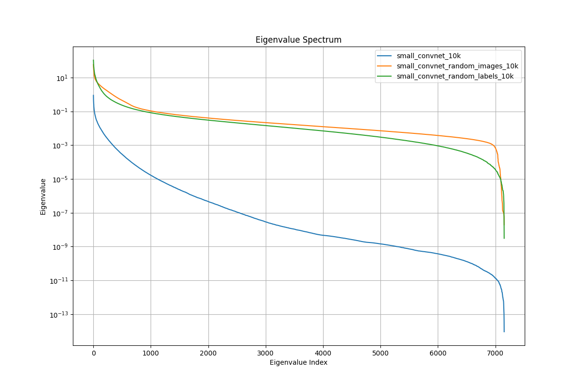
To provide our own evidence, we performed the following simple experiment, which only required a personal laptop for the computations. We used the MNIST dataset and trained the following relatively small convolutional neural network with 7154 parameters. The network had two convolutional layers with 3x3 kernels and two fully connected layers, all with ReLU nonlinearities, followed at the end by a softmax layer that produces a probability distribution over the labels. The architecture is described in Figure 1

Training was performed on three types of data: actual MNIST data, MNIST data with random labels, and data where the images themselves were random. The network was trained on 10000 samples so that the SGD algorithm converges even in the random cases, which require utilizing all parameters to fit the data. In Figure 2, we present the eigenvalue distribution of the empirical covariance matrix of the log-likelihood gradient (representing an empirical estimate of the FIM) for all the three cases: from the largest to the smallest, where the y-axis is plotted on a logarithmic scale. As can be clearly seen, for real data the eigenvalues drop quite rapidly to small values, whereas in the random cases, where all dimensions are utilized (with poor regret), the eigenvalues exhibit almost no decay. In addition, the gradients in the random cases are larger.