Universal cumulants and conformal invariance in annihilating random walks with pair deposition
Abstract
We consider annihilating random walks on the finite one-dimensional integer torus with deposition of pairs of particles, conditioned on an atypical jump activity. All cumulants of the activity, defined as the number of particle jumps up to some time , are obtained in closed form to leading order in system size at the critical point, where in the thermodynamic limit the conditioned process undergoes a phase transition in the universality class of the one-dimensional quantum Ising model in a transverse field. The generating function of the cumulants at a distance of order away from the critical point is proved to be given by two universal quantities, viz., by the central charge of the Virasoro algebra that characterizes the Ising universality class and by an explicit universal scaling function.
1 Laboratoire de Physique et Chimie Théoriques, Université de Lorraine, CNRS, F-54000 Nancy, France
2
Centro de Análise Matemática, Geometria e Sistemas Dinâmicos, Departamento de Matemática, Instituto Superior T’ecnico, Universidade de Lisboa, Av. Rovisco Pais 1, 1049-001 Lisboa, Portugal
Keywords: Annihilating random walks with pair deposition, large deviations, dynamical phase transition, quantum XY spin chain
1 Introduction
Large deviation theory provides a major source of insight into the properties of physical many-body systems, both in and out of thermal equilibrium. Prominent examples include dynamical Gibbs-non-Gibbs transitions [56] or fluctuation theorems [27] such as the celebrated Evans-Searles Theorem [22], the Jarzinski relation [22, 36], the Gallavotti-Cohen symmetry [25] and violations thereof [12, 30].
In the context of stochastic interacting particle systems (SIPS) large deviation properties are frequently addressed by conditioning the Markovian dynamics on some rare event [23, 17, 13, 40], in particular an atypical value of the particle current or of the activity, i.e., the number of particle jumps [42, 19, 10]. Away from the typical behavior of the process, dynamical phase transitions may occur [11, 26, 43, 35] that can only be understood when the full distribution of current and activity is considered. As noted in [38, 39], some such dynamical phase transitions are universal, i.e., independent of the microscopic details of the particle system and described by conformal field theory, a powerful tool in the study both of static equilibrium critical phenomena [20, 33, 16] and stochastic dynamics involving Schramm-Loewner evolution [24, 8, 15].
Specifically, at higher than typical activity the symmetric simple exclusion process (SSEP) [53, 45] defined on an integer torus of sites can be described in the thermodynamic limit by a conformal field theory with central charge of the Virasoro algebra [38] and critical exponents that are given by the Legendre parameter that is conjugate to the activity via Legendre transformation [40]. At maximal activity this becomes the field theory of free fermions which arises also when considering the density fluctuations of a Fermi fluid in one dimension which in turn are related to fluctuations of vicinal surfaces [54]. By appealing to universality one thus expects that independently of microscopic details of the model the same critical large-scale behaviour describes generic symmetric lattice gas models with one conservation law in the thermodynamic limit of infinite system size.
The universality hypothesis of large deviation properties found support some time ago when Appert et al. [6] showed by using the Bethe ansatz that the cumulants of the particle current and activity distribution of the SSEP defined on the integer torus with sites have universal finite-size scaling properties, i.e., universal large-scale behaviour when the limit of infinite system size and Legendre parameter is taken simultaneously. For the SSEP, is the phase transition point from a hyperuniform to a phase-separated regime [43, 35, 38] and is a scaling exponent. Also the current distribution in the totally asymmetric simple exclusion process exhibits universal features with dynamical exponent [1, 2, 11, 3, 4, 5]. This observation is intriguing and raises the question what other universality classes (if any) may exist and what universal scaling function would emerge.
Following this line of research, the study of universality classes for dynamical phase transition in SIPS was further pursued for the process of diffusion-limited pair annihilation and deposition (DLPAD). In this process particles are deposited in pairs in neighboring lattice sites and perform independent random walks, but annihilate instantly when two particles meet on the same site. There is a critical atypical activity, given by a non-zero Legendre parameter at which the process is described again by a conformal field theory [39], but unlike the conditioned SEP in the universality class of the critical one-dimensional quantum Ising model in a transverse field with central charge [33, 37].
It is the purpose of the present work to address the question of universal scaling functions for conditioned processes at a critical point and their link to conformal invariance rigorously by studying the cumulants of the activity of the DLDAP at the critical point. The main results of present work, established in Theorem 3.10 and Theorem 3.13, are an explicit computation of all cumulants to leading order in system size and the derivation of a universal generating function for the cumulants in the thermodynamic limit with distance from the critical point . The scaling properties are different from their counterparts in the SSEP that were obtained in [6]: The scaling function is different, the scaling exponent , characteristic for ballistic scaling, is different from the diffusive exponent for the SSEP, and the odd cumulants scale differently with system size.
With a view on future research along these lines we suggest that further universal properties and universality classes may be explored mathematically rigorously. As examples of interest we mention the DLDAP with non-periodic boundaries, related to the quantum Ising model in a transverse field with boundary fields [44, 48, 37], and the exclusion process with nearest neighbour jumps but a logarithmic long-range interaction [54, 49] which is closely related to Dyson’s Brownian motion [21] and the Calogero-Sutherland model [14, 55] which in turn all have an intimate well-established connection to Coloumb gases and random matrix theory via the circular unitary ensemble. Logarithmic interaction potentials play a role also in stochastic models of DNA denaturation [7, 34]. Thus understanding universality classes of activity cumulants may shed light on a large variety of problems of interest in different fields of probability theory and statistical physics, including applications.
This paper is organized as follows. In Sec. 2 we define the process in terms of its Markov generator and review its link to the quantum Ising chain in a transverse field which is used to prove the results. Also the activity is defined. In Sec. 3 first some further tools are presented and then the main results Theorem 3.10 and Theorem 3.13 as well as some special cases of these are stated and proved.
2 Diffusion-limited pair annihilation and deposition (DLPAD)
Informally, diffusion-limited pair annihilation and deposition is a Markov process where pairs of particles are deposited independently on neighboring sites of a lattice with a rate . These particles perform random walks with rate to a neighbouring site and whenever two particles meet at the same site they both annihilate instantly. Hence, at any positive time each site is occupied by at most one particle and, as noted in [9], the DLPAD starting with at most one particle per site is equivalent to a nonconservative exclusion process where (i) particles jump with rate to nearest neighbour sites provided the target site is empty, (ii) neighbouring pairs of particles are annihilated with rate , (iii) particle pairs are created with rate , provided the pair of target sites is empty.
This nonconservative exclusion process is a SIPS that was first studied in some detail in [28]. For this process reduces to diffusion-limited pair annihilation, also known as annihilating random walk, and for to pair annihilation and deposition which both have a long history of study, see e.g. [57, 47, 58] and references therein. In the present work both and are taken to be strictly positive. As lattice we consider the finite integer torus with sites and assume that the process starts with at most one particle per site.
2.1 Generator and invariant measure of the DLPAD
The lattice sites of the finite integer torus with sites are counted from to modulo . Each may be empty or occupied by at most one particle which is indicated by the occupation number . A complete configuration of the lattice is specified by the set of all occupation numbers . The locally flipped configuration is defined for a given configuration by the occupation numbers
| (2.3) |
and is used to define transitions from one configuration to another.
Definition 2.1
With the local transition rate
| (2.4) |
with strictly positive jump rate and strictly positive deposition rate the Markov chain on the state space defined by the generator
| (2.5) |
acting on bounded functions is called diffusion-limited pair annihilation and deposition (DLPAD).
Remark 2.2
Since particles are annihilated or deposited in pairs, the total particle number
| (2.6) |
is even or odd at all positive times. Hence the DLPAD is trivially nonergodic, with disjoint ergodic sectors with an even (+) or odd (-) number of particles respectively. We denote the respective state spaces by and the generators restricted to these state spaces by .
It was shown in [28] that the DLPAD is reversible w.r.t. the Bernoulli product measure
| (2.7) |
with the marginals
| (2.8) |
with particle density
| (2.9) |
For any non-zero deposition rate the density is in the range .
2.2 Intensity matrix and quantum XY chain
As detailed in [47, 58, 51], the intensity matrix (frequently called -matrix in the probabilistic literature [46]) defined by the generator of DLPAD has a natural representation in terms of the Hamiltonian operator of a non-Hermitian quantum spin chain. According to [46] the off-diagonal matrix elements of the intensity matrix are the transition rates
| (2.10) |
from a configuration to configuration of the DLPAD with the local transition rates defined in (2.4). The diagonal elements are given by
| (2.11) |
which expresses conservation of probability. The matrix with offdiagonal elements is a non-Hermitian matrix related to the Hamiltonian operator of the one-dimensional spin-1/2 quantum XY-chain in a transverse field [29] given by
| (2.12) |
with
| (2.13) | |||||
expressed in terms of the unit matrix and the spin-1/2 ladder operators and projectors acting on site , see [47, 51] for a review of the representation of the generators of stochastic interacting particle systems in terms of quantum spin chains and specifically [9] for a detailed derivation of (2.12) from the generator (2.5). Here we only mention that in this construction one uses the canonical basis vectors and of from which one constructs the tensor basis
| (2.14) |
of which is isomorphic to and which provides an isomorphism between the elements of the state space and the canonical basis vectors and their transposed vectors of . In slight abuse of language we call the quantum Hamiltonian of the process.
The projections on the even and odd particle sectors can be constructed in terms of the particle numebr operator , particle parity operator , and the projectors defined by
| (2.15) |
Then
| (2.16) |
yield the intensity matrices that define the Markov semigroup associated with the DLDAP in the even () and odd () sector respectively.
The link to the Hermitian quantum Hamiltonian operator of the one-dimensional spin-1/2 quantum XY-chain in a transverse field enables us to use various well-known results [33]. To this end, it is useful to introduce the spin operator defined by
| (2.17) |
and the parameters
| (2.18) |
2.3 Activity
2.3.1 Definition
The activity is defined as the total number of particle jumps in the DLPAD that have occured up to time , starting from some initial configuration with at most one particle on each site. Hence is a random number that is incremented by 1 whenever a particle jump with rate occurs and . Following the strategy outlined in [31], the evolution of can be captured by the joint process with state space defined by the generator
| (2.22) | |||||
for all and . Denoting expectations for this joint process with initial configuration by , the moment generating function of the activity is defined by
| (2.23) |
where is the Legendre parameter conjugate to the activity. Expressing the activity distribution in terms of the Legendre parameter is analogous to passing from a microcanonical ensemble for fixed to a canonical fluctuating ensemble [40].
As established in [17] this generating function can be expressed in terms of a tilted generator which for the DLPAD reads
| (2.24) |
acting on bounded functions defined on the original state space . One has
| (2.25) |
where the expectation is taken for the evolution defined by the tilted generator which does not conserve probability so that the expectation over the sum of all indicators is not equal to 1 but a non-trivial function of and .
2.3.2 Tilted intensity matrix
Associated with the tilted generator is the tilted intensity matrix and the tilted quantum Hamiltonian
| (2.26) | |||||
which is of the same form as the untilted quantum Hamiltonian (2.12) but with -dependent parameters. Replacing in the diagonal transformation matrix (2.19) the parameter by
| (2.27) |
therefore yields the transformed quantum Hamiltonian
| (2.28) |
where
| (2.29) |
and .
In terms of the tilted quantum Hamiltonian the moment generating function is given by
| (2.30) |
which follows from the discussion in [17] by using the matrix representation of the generator in the tensor basis (2.14) defined above. For the ground state of this Hamiltonian, discussed below, has a critical point
| (2.31) |
at a finite negative value of where the Ising phase transition referred to in the introduction occurs.
2.3.3 Cumulant generating function
As is extensive both in system length in time we consider the scaled activity with moment generating function and cumulant generating function . As in [6] we are interested in the asymptotic long-time behavior at fixed and where due to ergodicity the moment generating function and therefore also the cumulant generating function lose their dependence on the initial configuration except for the initial particle number parity. Thus we define for
| (2.32) |
and note the trivial property for .
The second point to observe is that since the state space is finite the tilted quantum Hamiltonian has a finite spectral gap in each sector defined by the projected quantum Hamiltonian with lowest eigenvalues denoted by . Since is extensive in system size it is natural to introduce the ground state energy per site . Then the limiting cumulant generating function of is in complete analogy to [6] given by
| (2.33) |
The ground state energy per site has been computed exactly using techniques based on the Jordan-Wigner transformation that expresses the spin lowering and raising operators appearing the quantum Hamiltonian into operators satisfying fermionic anticommutation relations [44]. This transformation leads to a many-body system of spinless free fermions that can be solved exactly using the techniques developed in [44] or, more straightforwardly, by the Cooper pair approach of [50] that by duality reduces the computation of the ground state energy of the many-body DLPAD to treating a collection of non-interacting two-state systems [52]. With the discrete dispersion relation [41, 39]
| (2.34) | |||||
| (2.35) | |||||
| (2.36) |
which satisfies the symmetry relation one gets [37, 39]
| (2.37) |
The cumulants are then given by
| (2.38) |
We recall that the first cumulant is the mean activity, the second cumulant is the variance, and the third cumulant is the third central moment.
Below we focus on the even sector at the critical point defined in (2.31) and to ease notation the superscript is dropped on all quantities considered below. In terms of the rates of the DLPAD and with the short-hand notation
| (2.39) |
we note that in terms of the rates and of the DLDAP
| (2.40) |
Since for the activity is trivially zero only needs to be considered. We introduce the normalized deposition rate which makes the overall time scale of the process. Without loss of generality we take which means that particles jump after an exponential random time with parameter . It is convenient to express the results for the critical point in terms of the complementary deposition rate
| (2.41) |
that appears frequently in the explicit formulas obtained below. We consider to be fixed and therefore omit the dependence of the cumulants and other functions on this quantity.
After these preparations we can state and prove the main results, all of which are based on taking judiciously chosen limits in (2.37). The proofs are all computational.
3 Critical cumulants
The general expression (2.37) yields the cumulant generating function
| (3.42) |
for the cumulants
| (3.43) |
at the critical point (2.31). To highlight the anticipated significance of the large- behaviour of the cumulants at the critical point the dependence on is written as an argument rather than a subscript.
3.1 Auxiliary Lemmas
For large system size, the leading order behaviour of the cumulant generating function evaluated at the critical point is captured by using the following Lemma.
Lemma 3.1
To the first subleading order in the trigonometric sums
| (3.44) |
are for and given by
| (3.45) |
Proof: By definition and binomial theorem
Using the geometric sum formula yields for and any finite
| (3.46) | |||||
The Taylor expansion
| (3.47) |
and observing that
then yields the two leading order terms
Since the sum over the binomial coefficients adds up to , the assertion (3.45) follows.
For an exact computation of the cumulants we use Faà di Bruno’s Theorem [18], which is a generalisation of the chain rule to arbitrary order, viz.,
| (3.48) |
with the Bell polynomials
| (3.49) |
where the sum is taken over all nonnegative integers such that
| (3.50) |
The cases relevant are the derivatives of a function of the exponential function and the square root of a quadratic function from which the cumulant generating function (3.42) and the cumulants (3.43) can be computed for any value of system size and of the expansion parameter .
Lemma 3.2
Let be times differentiable. Then
| (3.51) |
where
| (3.52) |
is the Stirling number of the second kind.
Proof: This follows from Faà di Bruno’s formula by using the combinatorial identity and the first constraint (3.50) in the definition of the Bell polynomials.
Lemma 3.3
Let be a quadratic polynomial with roots . Then for and
| (3.53) | |||||
where is the integer part function.
Proof: Since by assumption is a polynomial of order 2, only the Bell polynomials for which the summation is constrained to
| (3.54) |
appear in Faà di Bruno’s formula. Therefore , which yields
| (3.55) |
in the range or, equivalently,
| (3.56) |
which is the summation range in (3.53). Since
| (3.57) |
the assertion (3.53) follows.
3.2 Cumulant generating function at criticality
The cumulant generating function at the critical point is given by the sum (2.37) where at the critical point the dispersion relation (2.40) can be written as
| (3.58) |
in terms of the complementary deposition rate defined in (2.41). Here the trigonometric identities and are used and it is also taken into account that in the summation range the sine function does not change sign.
Proposition 3.4
To leading and subleading orders in system size the critical cumulant generating function in the range take the value
| (3.59) | |||||
| (3.60) |
with the constant
| (3.61) |
the sound velocity
| (3.62) |
and the central charge characterizing the Ising quantum chain in a transverse field.
This is essentially a well-established classical result [32]. A somewhat simpler proof is provided below.
3.3 Critical cumulants
Combining the two Lemmas 3.2 and 3.3 yields exact expressions for the cumulants for any value of . Here we are interested in the evaluation of the cumulants at the critical point. With the the coefficients
| (3.65) |
the expansion of the cumulant generating function (2.37) around the critical point reads
| (3.66) |
and (2.38) becomes
| (3.67) |
for all .
3.3.1 Exact expressions for the critical point
Proposition 3.5
Proof: With the quadratic function
| (3.69) |
of the variable the dispersion relation (2.36) is given by
| (3.70) |
By Lemma 3.2
| (3.71) |
where Lemma 3.3 yields for
| (3.72) | |||||
At the critical point one has
| (3.73) | |||||
| (3.74) | |||||
| (3.75) |
where the trigonometric identities and are used.
Remark 3.6
As seen below, only the Stirling numbers of the second kind
| (3.76) | |||||
| (3.77) |
are relevant for the asymptotic behaviour of the cumulants.
3.3.2 Asymptotic behaviour
(i) Critical mean activity
For any the mean activity is the first cumulant, i.e., the first derivative
| (3.78) |
of the cumulant generating function w.r.t. . Straightforward computation yields
| (3.79) |
At the critical point we have , i.e.,
| (3.80) |
Proposition 3.7
To leading and subleading order in the critical mean activity in the range is given by
| (3.81) |
with the asymptotic critical mean activity
| (3.82) |
(ii) Critical Variance
The variance of the activity at the critical point is the second cumulant, i.e.,
| (3.85) |
where the constants are given by (3.68).
Proposition 3.8
For the variance of the activity at the critical point is logarithmically divergent in and given by
| (3.86) |
to leading order in .
Proof: According to Proposition 3.5 one can write where
| (3.87) | |||||
| (3.88) |
The second term is of a form similar to the appearing in the expression (3.83) for the mean activity and yields by Lemma 3.1 a subleading contribution of order 1 to the variance. The key point in estimating the first term is a saddle-point argument: Because of the inverse power of the sine function in , the dominant contribution to the sum (3.67) comes from small arguments of the sine, i.e., from the integers that are small compared to . The second observation is that for fixed the expansion of the cosine so that the subleading terms can be neglected. On the other hand, for large values of , the factor containing the cosines is uniformly bounded, while the sine is of subleading order. This generates at most subleading terms which can be neglected. Consequently, the terms
| (3.89) |
with arbitrary but fixed values of the summation index yield the leading order contribution to the variance obtained from the leading behavior
| (3.90) |
of the sum over .
(iii) Critical skewness
By definition, the skewness
| (3.91) |
of the activity distribution at the critical point is given by the third cumulant and the variance. To compute the large- behaviour of the critical skewness we use Proposition 3.8 and compute the third cumulant.
Proposition 3.9
For the critical skewness vanishes as and is given by
| (3.92) |
to leading order in .
Proof: To arrive at (3.92) the leading behaviour of the third cumulant
| (3.93) |
needs to be determined. This follows entirely along the lines of the proof of the variance. The leading term in comes from and with in (3.68) which is the term proportional to . As in the case of the variance, this leads to a logarithmic divergence of in . Straighforward computation of the coefficient, given by taking the cosine function at value 1, yields
| (3.94) |
to leading order in which together with the definition (3.91) and the variance (3.86) yields (3.92).
(iv) General cumulants at the critical point
With the arguments used in the proofs of Propositions 3.7 - 3.9 and the exact result (3.68) of Proposition 3.5 we are now in a position to state and prove the main result of this Section.
Theorem 3.10
For the cumulants at the critical point are given to leading order in by
| (3.95) | |||||
| (3.96) | |||||
| (3.97) | |||||
| (3.98) | |||||
| (3.99) |
with the mean activity (3.82) and the rescaled cumulants
| (3.100) | |||||
| (3.101) |
given for by
| (3.102) | |||||
| (3.103) | |||||
| (3.104) | |||||
| (3.105) |
and the Riemann -function .
Proof: For the assertion is an immediate consequence of Proposition 3.7. The cases and are treated in Proposition 3.8 and in the proof of Proposition 3.9. For all higher cumulants the proof is analogous to the proof of the variance. The dominant contribution to the sum (3.67) comes from the term in (3.68) with the largest negative power of the sine-function, which corresponds for even cumulants for to and in the double sum (3.68) which is
| (3.106) |
with arbitrary but fixed values of the summation index . Expanding and the cosine functions to leading order one arrives at
One has for
The identity
| (3.107) |
Similar considerations show that for odd cumulants only the terms with and and yield the leading behaviour. Therefore with the identity
| (3.108) |
one finds
Corollary 3.11
For the cumulants and are of equal divergent order in so that for
| (3.109) |
Remark 3.12
With the convention the coefficients and are well-defined.
3.4 Universal cumulant generating function
To establish universality of the activity distribution near the critical point consider the function
| (3.110) |
which is well-defined through the Taylor expansion of the square root in .
Theorem 3.13
The function
| (3.111) |
with the sound velocity has the universal scaling limit
| (3.112) |
with the central charge and the parameter free scaling function .
Proof: By Proposition 3.5
Therefore
and by Theorem 3.10
| (3.113) |
On the other hand, by Taylor expansion one gets
| (3.114) |
The equality (3.112) then follows from the leading-order finite-size corrections (3.59) and (3.81).
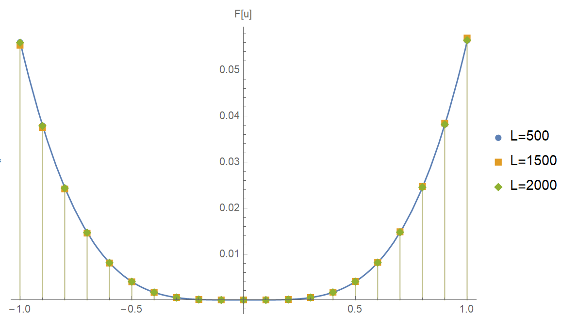
The theorem establishes a direct link between the cumulant generating function near the critical point and universal quantities at the critical point, obtained by substracting the leading non-universal contributions up to order two from the generating function for the cumulants of order 4 and higher. It can be recast as
| (3.115) |
Numerically, already moderately high system sizes reproduce the limiting behaviour, as shown in Fig. 1.
Remark 3.14
Consider the coefficients
| (3.116) |
and the function
| (3.117) |
By Taylor expansion of the square root one finds that
This generating function is non-universal since it depends on the microscopic parameter .
Acknowledgements
G.M.S. thanks the LPCT at the Université de Lorraine where part of this work was done, for kind hospitality. This work was supported by FCT (Portugal) through project UIDB/04459/2020, doi 10-54499/UIDP/04459/2020 and by the FCT Grants 2020.03953.CEECIND and 2022.09232.PTDC.
References
- [1] Arai, Y.: On the KPZ Scaling and the KPZ Fixed Point for TASEP. Math. Phys. Anal. Geom. 27, 4 (2024).
- [2] J. Baik, A. Prokhorov, and G. L. F. Silva, Differential Equations for the KPZ and Periodic KPZ Fixed Points, Commun. Math. Phys. 401 (2023) 1753–1806
- [3] Corwin, I.: The Kardar-Parisi-Zhang equation and universality class, Rand. Mat.: Theo. Appl. 1, 1130001 (2012).
- [4] K. Matetski, J. Quastel, and D. Remenik The KPZ fixed point. Acta Math. 227, 115–203 (2021).
- [5] M. Prähofer and H. Spohn, Exact scaling function for one-dimensional stationary KPZ growth. J. Stat. Phys. 115, 255–279 (2004).
- [6] Appert C., Derrida B., Lecomte V., Van Wijland, F.: Universal cumulants of the current in diffusive systems on a ring. Phys. Rev. E 78, 021122 (2008).
- [7] A. Bar, Y. Kafri, and D. Mukamel, Dynamics of DNA melting, J. Phys.: Condens. Matter 21 034110 (2009).
- [8] M. Bauer and D. Bernard, Conformal Field Theories of Stochastic Loewner Evolutions, Commun. Math. Phys. 239, 493–521 (2003)
- [9] V. Belitsky and G.M. Schütz, Duality, supersymmetry and non-conservative random walks, J. Stat. Mech. 2019, 054004, (2019).
- [10] Bertini, L., De Sole, A., Gabrielli, D., Jona Lasinio, G., Landim, C.: Macroscopic fluctuation theory. Rev. Mod. Phys. 87, 593–636 (2015).
- [11] T. Bodineau and B. Derrida, Distribution of current in nonequilibrium diffusive systems and phase transitions, Phys. Rev. E 72, 66110 (2005).
- [12] F. Bonetto, G. Gallavotti, A. Giuliani, F. Zamponi, Chaotic Hypothesis, Fluctuation Theorem and Singularities J. Stat. Phys. 123, 39–54 (2006).
- [13] A.N. Borodin, Stochastic Processes, Birkhauser, Springer International Publishing, Switzerland (2017).
- [14] F. Calogero, Ground State of a One‐Dimensional N‐Body System, J. Math. Phys. 10, 2197–2000 (1969).
- [15] J. Cardy, SLE(kappa,rho) and Conformal Field Theory, arXiv:math-ph/0412033v2 (2004).
- [16] J.L. Cardy, Conformal Field Theory and Statistical Mechanics, in: Exact Methods in Low-dimensional Statistical Physics and Quantum Computing: Lecture Notes of the Les Houches Summer School: Volume 89, July 2008, J. Jacobsen, S. Ouvry, V. Pasquier, D. Serban, and L. Cugliandolo (eds.) (Oxford University Press, Oxford, 2010).
- [17] R. Chetrite, H. Touchette, Nonequilibrium Markov processes conditioned on large deviations, Ann. Henri Poincaré 16, 2005-2057 (2015).
- [18] L. Comtet, Advanced Combinatorics (Springer, Dordrecht, 1974).
- [19] Derrida, B.: Non-equilibrium steady states: fluctuations, large deviations of the density, of the current J. Stat. Mech. P07023 (2007).
- [20] P. Di Francesco, P. Mathieu, and D. Sénéchal, Conformal Field Theory (Springer, New York, 1997)
- [21] F.J. Dyson, A Brownian-Motion Model for the Eigenvalues of a Random Matrix, J. Math. Phys. 3, 1191–1198 (1962).
- [22] D.J. Evans, D.J. Searles, Equilibrium microstates which generate second law violating steady states, Phys. Rev. E 50, 1645–1648 (1994).
- [23] J. Feng, T.G. Kurtz: Large Deviations for Stochastic Processes, AMS, 410 pp (2006)
- [24] Conformal fields, restriction properties, degenerate representations and SLE, C. R. Acad. Sci. Paris I 335, 947–952 (2002)
- [25] Gallavotti, G. and Cohen, E G D.: Dynamical ensembles in stationary states, J. Stat. Phys. 80, 931–970 (1995)
- [26] J.P. Garrahan, R.L. Jack, V. Lecomte, E. Pitard, K. van Duijvendijk, and F. van Wijland, First-order dynamical phase transition in models of glasses: an approach based on ensembles of histories, J. Phys. A: Math. Theor. 42 075007 (2009).
- [27] P. Gaspard, The power of fluctuation relations, (Cambridge University Press, Cambridge, 2022)
- [28] M. D. Grynberg, T.J. Newman, and R. B. Stinchcombe, Exact solutions for stochastic adsorption-desorption models and catalytic surface processes, Phys. Rev. E 50, 957–971 (1994).
- [29] M. D. Grynberg and R. B. Stinchcombe, Dynamics of adsorption-desorption processes as a soluble problem of many fermions, Phys. Rev. E 52, 6013–6024 (1995).
- [30] Harris, R J., Rákos, A. and Schütz, G M.: Breakdown of Gallavotti-Cohen symmetry for stochastic dynamics, Europhys. Lett. 75, 227–233 (2006)
- [31] R.J. Harris and G.M. Schütz Fluctuation theorems for stochastic dynamics J. Stat. Mech. 2007, P07020 (2007)
- [32] M. Henkel, Finite-size scaling and universality in the spectrum of the quantum ising chain. I. Periodic and antiperiodic boundary condition, J. Phys. A: Math. Gen. 20, 995–1010 (1987)
- [33] M. Henkel, Conformal Invariance and Critical Phenomena (Springer, Berlin, 1999).
- [34] O. Hirschberg, D Mukamel, and G. M. Schütz, Approach to equilibrium of diffusion in a logarithmic potential, Phys. Rev. E 84, 041111 (2011).
- [35] R.L. Jack, I.R. Thompson, and P. Sollich, Hyperuniformity and Phase Separation in Biased Ensembles of Trajectories for Diffusive Systems Phys. Rev. Lett. 114, 060601 (2015).
- [36] Jarzynski, C.: Nonequilibrium equality for free energy differences, Phys. Rev. Lett. 78, 2690–2693 (1997)
- [37] D. Karevski, Surface and bulk critical behaviour of the XY chain in a transverse field, J. Phys. A, Math. Gen. 33, L313–L317 (2000).
- [38] D. Karevski and G. M. Schütz, Conformal invariance in driven diffusive systems at high currents, Phys. Rev. Lett. 118, 030601 (2017).
- [39] D. Karevski and G. M. Schütz, Dynamical phase transitions in annihilating random walks with pair deposition, J. Phys. A: Math. Theor. 55, 394005 (2022).
- [40] C. Monthus, Microcanonical conditioning of Markov processes on time-additive observables, J. Stat. Mech. 2022, 023207 (2022).
- [41] Th. Niemeijer, Some exact calculations on a chain of spins 1/2, Physica 36, 377–419 (1967).
- [42] J.L. Lebowitz and H. Spohn, A Gallavotti-Cohen-Type Symmetry in the Large Deviation Functional for Stochastic Dynamics, J. Stat. Phys. 95, 333–365 (1999).
- [43] V. Lecomte, J.P. Garrahan, and F. van Wijland, Inactive dynamical phase of a symmetric exclusion process on a ring, J. Phys. A: Math. Theor. 45, 175001 (2012).
- [44] E. Lieb, T. Schultz, D. Mattis, Two Soluble models of an antiferromagnetic chain, Ann. Phys. 16, 407–466 (1961).
- [45] Liggett, T.M.: Stochastic Interacting Systems: Contact, Voter and Exclusion Processes. Springer, Berlin (1999).
- [46] T.M. Liggett, Continuous Time Markov Processes: An Introduction, Graduate Studies in Mathematics Vol. 113, American Mathematical Society, Rhode Island (2010).
- [47] P. Lloyd, A. Sudbury, and P. Donnelly, Quantum operators in classical probability theory: I. “Quantum spin” techniques and the exclusion model of diffusion, Stoch. Proc. Appl. 61, 205–221 (1996).
- [48] P. Pfeuty, The one-dimensional Ising model with a transverse field, Ann. Phys. (NY) 57, 79–90 (1970).
- [49] V. Popkov, D. Simon, and G.M. Schütz, ASEP on a ring conditioned on enhanced flux, J. Stat. Mech. 2010, P10007 (2010).
- [50] G.M. Schütz, Diffusion-annihilation in the presence of a driving field. J. Phys. A: Math. Gen. 28, 3405–3415 (1995).
- [51] Schütz, G.M.: Fluctuations in Stochastic Interacting Particle Systems. In: Giacomin G., Olla S., Saada E., Spohn H., Stoltz G. (eds), Stochastic Dynamics Out of Equilibrium. IHPStochDyn 2017. Springer Proceedings in Mathematics & Statistics, vol 282. (Springer, Cham, 2019).
- [52] G.M. Schütz, Duality from integrability: annihilating random walks with pair deposition, J. Phys. A: Math. Theor. 53, 355003 (2020).
- [53] F. Spitzer, Interaction of Markov processes, Adv. Math. 5, 246–290, (1970).
- [54] H. Spohn, Bosonization, vicinal surfaces, and hydrodynamic fluctuation theory, Phys. Rev. E 60, 6411–6420 (1999).
- [55] B. Sutherland, Exact Results for a Quantum Many-Body Problem in One Dimension. II, Phys. Rev. A 5, 1372–1376 (1972).
- [56] A.C.D. van Enter, R. Fernandez, F. den Hollander, and F. Redig: A large-deviation view on dynamical Gibbs-non-Gibbs transitions, Moscow Math. Journal 10, 687–711 (2010)
- [57] A. W. Sudbury and P. Lloyd, “Quantum Operators in Classical Probability Theory II: The Concept of Duality in Interacting Particle Systems,” Annals of Probability 23 (4), 1816–1830 (1995).
- [58] G. M. Schütz, “Exactly Solvable Models for Many-Body Systems Far from Equilibrium,” in Phase Transitions and Critical Phenomena, Vol. 19, edited by C. Domb and J. L. Lebowitz (Academic Press, London, 2001), pp. 1–251.