Bayesian adaptive randomization in the I-SPY2.2 sequential multiple assignment randomized trial

Abstract

[Abstract]The I-SPY2 phase 2 clinical trial is a long-running platform trial evaluating neoadjuvant treatments for locally advanced breast cancer, assigning subjects to tumor subtype-specific experimental agents via a response-adaptive randomization algorithm that updates randomization probabilities based on accruing evidence of efficacy. Recently, I-SPY2 has been reconfigured as a sequential multiple assignment randomized trial (SMART), known as I-SPY2.2, in which subjects who are predicted to not achieve a satisfactory response to an initial assigned therapy are re-randomized to a second subtype-specific treatment followed by standard rescue therapy if a satisfactory response is not predicted. The I-SPY2.2 SMART thus supports evaluation of entire treatment regimes that dictate the choice of treatments at each stage on the basis of the outcome pathological complete response (pCR). The transition of I-SPY2 to a SMART required development of a trial-specific response-adaptive randomization scheme in which randomization probabilities at each stage are updated based on evolving evidence on the efficacy of full regimes, so as to skew probabilities toward treatments involved in regimes that the current evidence suggests are optimal in the sense of maximizing the probability of pCR. The approach uses Thompson sampling, which updates randomization probabilities based on the posterior probability that treatments are implicated in optimal regimes. We present the proposed algorithm and empirical studies that demonstrate it improves within-trial regime-specific pCR rates and recommends optimal regimes at similar rates relative to uniform, nonadaptive randomization.

1 Introduction

The I-SPY2 phase 2 trial in patients with stage II and III high-risk breast cancer is one of the first multicenter adaptive platform trials^{1, 2} and is widely acknowledged as having had a major impact on both trial design and the treatment of breast cancer. Over more than a decade, I-SPY2 has evaluated simultaneously multiple investigational neoadjuvant agents targeted to biologically-defined patient subtypes on the basis of the early endpoint of pathological complete response (pCR) and identified agents having high probability to be successful in phase 3 trials. Hallmarks of I-SPY2 are its use of response-adaptive randomization^{3, 4, 5} to preferentially assign subjects to experimental agents demonstrating efficacy within a subject’s breast cancer subtype and its role in establishing pCR as a strong predictor of event free survival⁶ and markedly improving the standard of care in some subtypes. The increases in subtype-specific rates of pCR demonstrated in I-SPY2 have helped inspire a change in focus toward development of agents achieving the same efficacy with fewer adverse effects.

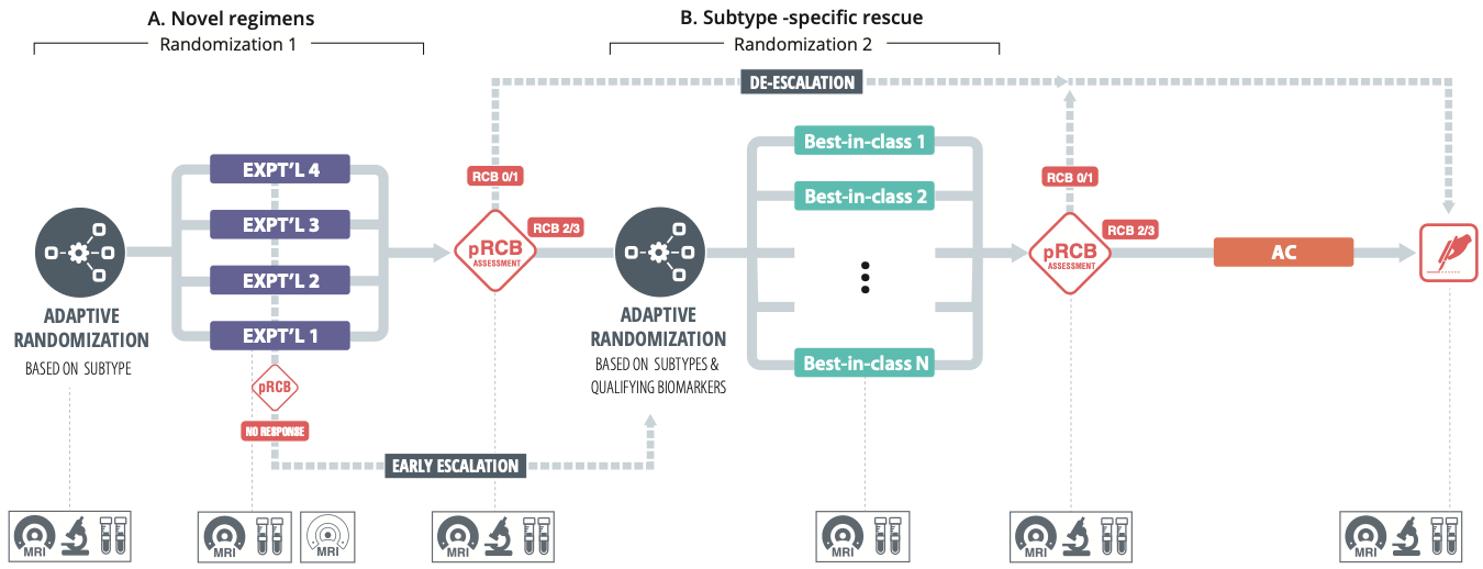
Figure 1: I-SPY2.2 SMART schema for a given subtype.

This interest in novel targeted agents with similar efficacy to current “best-in-class” agents but offering potential reduction in toxicities has inspired a reconfiguration of the I-SPY2 as a sequential multiple assignment randomized trial (SMART)⁷, I-SPY2.2^{8, 9}, with the goal of evaluating new agents while allowing participants who are deemed likely to have a poor response to an experimental agent the opportunity to switch to a best-in-class agent for their tumor subtype. Specifically, in I-SPY2.2, upon being classified as belonging to a given tumor subtype, subjects follow the schema depicted in Figure 1 involving two randomizations and three stages or “blocks” of neoadjuvant therapy as follows. Within a subtype, subjects are initially randomized to subtype-specific novel experimental agents at stage 1 of the SMART, referred to by the investigators as “Block A.” During Block A, a subject’s potential response to the assigned agent is evaluated every 3 to 6 weeks using an imaging biomarker, functional tumor volume (FTV), determined by breast MRI. At the completion of therapy (end of Block A; roughly 12 weeks), biopsy of the tumor bed and/or lymph nodes is performed, and an algorithm referred to as “preRCB,” which incorporates FTV and biopsy information, is used to evaluate the subject’s probability of pCR (pCR can be confirmed only via surgical resection). Subjects for whom the probability is sufficiently high, to whom we refer as “responders,” are given the option to proceed to surgery without further treatment (so meet the criteria for treatment de-escalation), at which time pCR status is ascertained. Those not meeting the criteria (“nonresponders” to initially assigned therapy) are recommended to continue to stage 2 of the SMART, referred to as “Block B,” as are subjects who are deemed earlier in Block A to be on a trajectory for poor response on the basis of FTV (so eligible for early treatment escalation), where they are re-randomized to a subtype-specific “best-in-class” agent. Again, potential response is evaluated during Block B via FTV, and at the end of Block B, following biopsy, responders meeting the preRCB de-escalation criteria are given the option to proceed to surgery, at which point pCR status is determined definitively. Nonresponders to assigned Block B therapy as indicated by preRCB (or by a poor trajectory of earlier repeated FTV evaluations) are recommended to receive rescue chemotherapy, Adriamycin (doxorubicin) and cyclophosphamide (AC), following which pCR status is ascertained. For convenience later, we refer to this further therapy for stage 2/Block B nonresponders as “stage 3,” although it is not a true stage of the SMART, as there is no randomization conducted. Thus, in I-SPY2.2, a participant’s pCR outcome is determined at the end of stage 1, end of stage 2, or end of stage 3, depending on whether or not she proceeds to surgery at the end of each stage. Although in this article we restrict attention to the foregoing SMART design with two stages of randomization, the approach we propose can be generalized to a SMART involving more than two stages, which, in I-SPY2.2, would allow incorporation of a true stage 3 with randomization among AC and additional rescue options (“Block C”).

A key feature of I-SPY2.2 is that the likelihood that subjects receive ineffective or unnecessary therapy is minimized, so that exposure to potential toxicities associated with unneeded treatment is limited. Thus, I-SPY2.2 offers participants the opportunity to avoid overtreatment in the event that they are responders and to receive further, subtype-specific therapy if they are not.

As with any SMART, the I-SPY2.2 design allows evaluation of entire treatment strategies, or treatment regimes,^{10, 11} that dictate how therapies should be given sequentially if needed. The design of a SMART induces a particular set of treatment regimes, referred to as the design’s embedded regimes, which follow naturally from the randomization structure. In I-SPY2.2, within a specific subtype, which determines the feasible stage 1/Block A and stage 2/Block B options, an example of an embedded regime is “Give experimental therapy 1; if the patient does not proceed to surgery by the end of Block A, give best-in-class therapy 3 followed by AC if the patient does not proceed to surgery by the end of Block B.” Later, we use the shorthand $\{1,3\}$ to denote this regime. Evaluation of entire subtype-specific embedded regimes is aligned with the goals of the investigators to advance precision oncology through optimization of choice of sequential, targeted therapies based on a patient’s response.

Given the history of the successful use of response-adaptive randomization in I-SPY2, a key goal of the reconfiguration to a SMART in I-SPY2.2 was implementation of a response-adaptive randomization scheme to update randomization probabilities at each stage to give greater weight to treatments that appear more efficacious based on accrued information from previous subjects in the trial. In conventional, single-stage randomized clinical trials (RCTs), adaptive randomization has been argued to have the ethical benefit of improving within-trial outcomes¹², and, while there can be a loss of efficiency of post-trial inference ¹³, this concern is less critical in multi-arm trials ¹⁴. However, adaptive randomization is much less developed for SMARTs, which involve multiple randomizations, than for conventional RCTs, with only a few methods available ^{15, 16, 17, 18}. Accordingly, we developed a study-specific response-adaptive randomization approach for I-SPY2.2. The approach uses Thompson sampling ¹⁹, a well-known algorithm that bases randomization probabilities on the posterior probabilities that treatment options are optimal and that has been a popular basis for response-adaptive randomization in conventional RCTs, particularly in oncology ^{20, 21}. The proposed method, which is now in use in the ongoing I-SPY2.2 SMART, is based on identifying for each subtype the subtype-specific embedded regime that currently maximizes the probability of achieving pCR. Owing to the unique features of I-SPY2.2, identifying this regime is straightforward and leads to a computationally simple strategy for updating approximate posterior probabilities of the candidate treatments at each stage of the SMART being optimal based on the accrued data from the trial and thus updated randomization probabilities for each treatment option at each stage.

In this article, we present the rationale for and derivation and implementation of the proposed I-SPY2.2 SMART response-adaptive randomization strategy and demonstrate its performance via empirical studies. In Section 2, we review Thompson sampling and fundamentals of SMARTs and treatment regimes. We develop the statistical framework and response-adaptive randomization scheme in Section 3. Section 4 presents results of simulation studies to evaluate the approach.

2 Background

2.1 Thompson sampling

The central idea of Thompson sampling is that the randomization probability for a treatment should be based on the degree of belief that the treatment is optimal among the possible options. The degree of belief typically is represented by the posterior probability that the treatment is optimal in the sense that it optimizes expected outcome ^{19, 22, 23}. In I-SPY2 and I-SPY2.2, with the binary outcome pCR, expected outcome is the probability of achieving pCR. Accordingly, in a conventional, single-stage clinical trial like I-SPY2, under Thompson sampling, as data accrue, the randomization probability for a given treatment option $a$ in a set of possible options $\mathcal{A}$, given the accrued data $\mathcal{D}$ to that point, is ordinarily taken to be related to the posterior probability $\rho(a\mid\mathcal{D})$ that $a$ optimizes expected outcome among all options in $\mathcal{A}$. More precisely, letting $\pi(a\mid\mathcal{D})$ denote the randomization probability based on the accrued data, $\pi(a\mid\mathcal{D})$ is usually linked to the posterior probability via a monotone function. A sensible and popular choice that strikes a balance between the posterior probability itself and uniform randomization²⁴ is to take

$$\pi(a\mid\mathcal{D})=\frac{\rho(a\mid\mathcal{D})^{\psi}}{\sum_{a^{\prime}\in\mathcal{A}}\rho(a^{\prime}\mid\mathcal{D})^{\psi}},$$ (1)

where $0\leq\psi\leq 1$ is a damping contant such that $\psi=1$ corresponds to taking $\pi(a\mid\mathcal{D})=\rho(a\mid\mathcal{D})$ and $\psi=0$ yields uniform randomization. As data accumulate, the randomization probability for an efficacious (inefficacious) treatment will increase (decrease) toward 1 (0), so that more (fewer) subjects will receive it. Taking $\psi$ equal to or close to 1 can result in aggressive adaptation and randomization probabilities approaching 1 or 0 for efficacious or inefficacious treatments, respectively, which can limit exploration of all options in $\mathcal{A}$. Thus, an intermediate value for $\psi$ strictly less than 1 may be a more practical choice. It is also possible to take $\psi$ to be time dependent, $\psi_{t}$, to allow the aggressiveness of adaptation to change with time.

In Section 3, we use the principle of Thompson sampling based on the posterior probability that an entire embedded treatment regime or stage 2 treatment option is optimal in the sense of maximizing the probability of pCR to derive adaptive randomization probabilities for subjects entering I-SPY2.2 at stage 1 or advancing to stage 2.

2.2 Treatment regimes and SMARTs

Generically, a treatment regime is a sequence of $K$ decision rules corresponding to $K$ decision points (stages) at which treatment decisions are to be made, where each rule takes a subject’s history of information to that point as input and outputs a recommended treatment option from among the available options. As an example, consider the regimes embedded in I-SPY2.2 in Section 1, for which $K=2$. For a given subtype $s$, $s=1,\ldots,\mathcal{S}$, stage 1 treatment option $a_{1}$ in the set of possible options $\mathcal{A}_{1,s}$, and stage 2 treatment option $a_{2}$ in the set of possible options $\mathcal{A}_{2,s}$, a subtype-specific embedded regime has rule corresponding to stage 1 “Give $a_{1}$” and rule corresponding to stage 2 “If the patient does not proceed to surgery during/after receiving $a_{1}$, give $a_{2}$ followed by AC if the patient does not proceed to surgery during/after receiving $a_{2}$.” These rules do not take into account additional information that may be available on an individual at each decision point beyond surgery status in the stage 2 rule. It is possible to specify regimes with more complex rules, where the rule at stage $k$ can incorporate both baseline patient variables and accrued covariate information up to stage $k$. There is a vast literature on estimating the expected outcome that would be achieved if the patient population were to follow the rules of a regime, referred to as the value of the regime; and on estimating an optimal regime, one that would lead to the most beneficial expected outcome/value in the population if the population were to follow its rules, from suitable data. See, for example, Tsiatis et al. (2020)¹¹ for a general account.

Just as the conventional RCT is the accepted study design for evaluating treatment effects based on a specified health outcome, the SMART, in which participants are randomized at each stage to the set of available treatment options, is the gold standard for evaluation of treatment regimes on the basis of a given outcome. Interest often focuses on the set of embedded regimes, which can be viewed as representing different “treatment sequences,” and on determining the optimal embedded regime, that leading to the most beneficial expected outcome. Strictly speaking, it is possible that there is more than one embedded regime achieving the same, most beneficial expected outcome and thus more than one optimal regime; for simplicity, we downplay this possibility and refer to “the” optimal embedded regime.

In I-SPY2.2, the binary outcome is the indicator of achieving pCR during the trial period. Thus, for each subtype, the optimal embedded regime is that maximizing the overall probability of pCR. A critical concept in evaluation of treatment regimes is that of delayed effects; namely, a treatment option selected at an earlier stage may have implications for which options should be selected at subsequent stages. For example, a Block A agent may potentiate the effect of a Block B agent given to patients not proceeding to surgery after Block A, so that the Block A option maximizing the probability of pCR at stage 1 only may not be part of the regime leading to the maximum pCR rate overall. Intuitively, then, an adaptive randomization strategy should determine updated randomization probabilities so that possible delayed effects are taken into account. This objective can be achieved by basing the randomization probability for a given option at each stage on the probability that the option is part of an entire optimal embedded regime. Thus, in contrast to some approaches for two-stage SMARTs that base the probabilities at stage 1 myopically on response status at the end of stage 1^{16, 18}, the response-adaptive randomization approach we propose for I-SPY2.2 in the next section is based on identifying optimal embedded regimes for each subtype at each update of the randomization probabilities.

3 Bayesian adaptive randomization in the I-SPY2.2 SMART

3.1 Statistical framework

As is standard for conventional RCTs, we assume that subjects enter I-SPY2.2 according to a completely random process over a planned accrual period, which we take for definiteness to be 30 months, so that subjects enter the SMART in a staggered fashion. For a given subject, upon entry, let $S$ be the subject’s subtype, and, if $S=s$, with $\mathcal{A}_{1,s}$ the set of stage 1/Block A subtype $s$-specific novel experimental therapies, let $A_{1}$ be the option from $\mathcal{A}_{1,s}$ to which the subject is randomized. By approximately 12 weeks, whether or not a subject is a responder is determined. Ideally, all subjects deemed responders would proceed to surgery; however, some responders may refuse and subjects deemed nonresponders may choose to proceed to surgery even though they are not recommended to do so. Accordingly, we take an intention-to-treat perspective and let $R_{1}=1$ if the subject proceeds to surgery and 0 if not. If $R_{1}=1$, the subject’s true pCR status at the end of stage 1, $Y_{1}$, is ascertained, where $Y_{1}=1(0)$ indicates that the subject did (did not) achieve pCR, and no further data are collected on the subject. If $R_{1}=0$, the subject advances to stage 2/Block B and is randomized to a best-in-class therapy $A_{2}$ from among the set $\mathcal{A}_{2,s}$ of such therapies. By approximately 12 weeks, whether or not the subject is a responder is determined; if the subject proceeds to surgery, $R_{2}=1$, and $R_{2}=0$ otherwise. If $R_{2}=1$, the subject’s true pCR status at the end of stage 2, $Y_{2}\in\{0,1\}$, is ascertained, and no further data are collected on the subject. At both stages 1 and 2, there is an approximate 1 week delay between when $R_{1}=1$ and $R_{2}=1$ are observed and surgery takes place and determination of $Y_{1}$ and $Y_{2}$ is made. If $R_{2}=0$, the subject receives AC (“stage 3”), and after approximately 12 weeks true pCR status $Y_{3}\in\{0,1\}$ is ascertained. Note that $Y_{k}$, $k=1,2$, is observed only if $R_{k}=1$, and $Y_{3}$ is observed only if a subject has $R_{1}=R_{2}=0$. The observed data on a subject can be summarized as

$$\mathcal{O}=\{S,A_{1},R_{1},Y_{1}I(R_{1}=1),A_{2}I(R_{1}=0),R_{2}I(R_{1}=0),Y_{2}I(R_{1}=0,R_{2}=1),Y_{3}I(R_{1}=0,R_{2}=0)\},$$ (2)

and the primary outcome of interest, recording whether or not pCR is achieved during the trial, is determined by (2) as $Y=Y_{1}I(R_{1}=1)+Y_{2}I(R_{1}=0,R_{2}=1)+Y_{3}I(R_{1}=0,R_{2}=0)$, the pCR status ascertained when surgery takes place. Note that only one of $Y_{1},Y_{2},Y_{3}$ is observed on a given subject, depending on surgery status.

For a subject of subtype $s$, define the following quantities. For $a_{1}\in\mathcal{A}_{1,s}$, let

$$\theta_{1,s}(a_{1})=P(R_{1}=1\mid S=s,A_{1}=a_{1}),\hskip 7.22743pt\gamma_{1,s}(a_{1})=P(Y_{1}=1\mid S=s,A_{1}=a_{1},R_{1}=1),$$ (3)

the conditional probability that a subject of subtype $s$ who receives treatment $a_{1}\in\mathcal{A}_{1,s}$ proceeds to surgery at stage 1 and the conditional probability that such a subject achieves pCR at stage 1, respectively. Similarly, for $a_{2}\in\mathcal{A}_{2,s}$, let

$$\theta_{2,s}(a_{1},a_{2})=P(R_{2}=1\mid S=s,A_{1}=a_{1},R_{1}=0,A_{2}=a_{2}),\hskip 5.05942pt\gamma_{2,s}(a_{1},a_{2})=P(Y_{2}=1\mid S=s,A_{1}=a_{1},R_{1}=0,A_{2}=a_{2},R_{2}=1).$$ (4)

Finally, let

$$\gamma_{3,s}(a_{1},a_{2})=P(Y_{3}=1\mid S=s,A_{1}=a_{1},R_{1}=0,A_{2}=a_{2},R_{2}=0).$$ (5)

Denote by the shorthand $\{a_{1},a_{2}\}$ the subtype $s$-specific embedded regime “Give $a_{1}$; if the patient does not proceed to surgery during/after receiving $a_{1}$, give $a_{2}$ followed by AC if the patient does not proceed to surgery during/after $a_{2}$” for all possible pairs $(a_{1},a_{2})\in\mathcal{A}_{1,s}\times\mathcal{A}_{2,s}$. Then it can be shown that the probability of achieving pCR if the population of subjects of subtype $s$ were to follow regime $\{a_{1},a_{2}\}$, that is, the value of regime $\{a_{1},a_{2}\}$, is given by

$$\mu_{s}(a_{1},a_{2}) =\theta_{1,s}(a_{1})\gamma_{1,s}(a_{1})+\{1-\theta_{1,s}(a_{1})\}\theta_{2,s}(a_{1},a_{2})\gamma_{2,s}(a_{1},a_{2})$$ (6)

$$+\{1-\theta_{1,s}(a_{1})\}\{1-\theta_{2,s}(a_{1},a_{2})\}\gamma_{3,s}(a_{1},a_{2}).$$

The expression (6) is intuitive and can be derived formally via the g-computation algorithm; e.g., see Section 5.4 of Tsiatis et al. (2020)¹¹. For convenience later, denote the entire set of probabilities involved in (6) for all possible options in $\mathcal{A}_{1,s}$ and $\mathcal{A}_{2,s}$ as

$$\Theta_{1,s}=\{\gamma_{1,s}(a_{1}),\gamma_{2,s}(a_{1},a_{2}),\gamma_{3,s}(a_{1},a_{2}),\theta_{1,s}(a_{1}),\theta_{2,s}(a_{1},a_{2});\,\,\,(a_{1},a_{2})\in\mathcal{A}_{1,s}\times\mathcal{A}_{2,s}\}.$$

From (6), for subtype $s$, the optimal embedded regime is $\{a_{1,s}^{opt},a_{2,s}^{opt}\}$, where $a_{1,s}^{opt}$ and $a_{2,s}^{opt}$ jointly maximize $\mu_{s}(a_{1},a_{2})$ in $a_{1}$ and $a_{2}$. It is straightforward to determine $a_{1,s}^{opt}$ and $a_{2,s}^{opt}$ by evaluating (6) at all of the (finite number of) possible combinations of options in $\mathcal{A}_{1,s}$ and $\mathcal{A}_{2,s}$. Note that $a_{1,s}^{opt}$ and $a_{2,s}^{opt}$ depend on $\Theta_{1,s}$. These developments suggest that the optimal strategy for a subject of subtype $s$ entering the SMART at any time during the accrual period and requiring a stage 1 treatment assignment would be to assign the subject to $a_{1,s}^{opt}$, the stage 1 option associated with regime $\{a_{1,s}^{opt},a_{2,s}^{opt}\}$ currently thought to be optimal and thus leading to the highest probability of achieving pCR during the trial.

Consider a subject of subtype $s$ already in the trial for whom $R_{1}=0$, so who is eligible to receive a stage 2 treatment option, and suppose the subject already received a particular option $a_{1}$ at stage 1, which may or may not be currently thought to be optimal in the sense of being part of an optimal regime as above. Analogous to the above, the optimal strategy for such a subject, given that $a_{1}$ has already been administered, would be to assign the subject the option $a_{2,s}^{opt}(a_{1})\in\mathcal{A}_{2,s}$ that maximizes in $a_{2}$ the probability of achieving pCR if the population were to receive this particular $a_{1}$ at stage 1 and then $a_{2}$ at stage 2, given by

$$\mu_{2,s}(a_{1},a_{2})=\theta_{2,s}(a_{1},a_{2})\gamma_{2,s}(a_{1},a_{2})+\{1-\theta_{2,s}(a_{1},a_{2})\}\gamma_{3,s}(a_{1},a_{2}).$$ (7)

Again, it is straightforward to determine $a_{2,s}^{opt}(a_{1})$ by evaluating (7) at each of the options in $\mathcal{A}_{2,s}$. As above, for convenience, for a given $a_{1}$, denote the set of probabilities involved in (7), which are a subset of those in $\Theta_{1,s}$ for the given $a_{1}$, as

$$\Theta_{2,s}(a_{1})=\left\{\gamma_{2,s}(a_{1},a_{2}),\gamma_{3,s}(a_{1},a_{2}),\theta_{2,s}(a_{1},a_{2});\,\,\,a_{2}\in\mathcal{A}_{2,s}\right\}.$$

Analogous to the above, $a_{2,s}^{opt}(a_{1})$ depends on $\Theta_{2,s}(a_{1})$.

In the next section, these observations motivate the proposed adaptive randomization scheme.

3.2 Adaptive randomization scheme

In principle, the proposed adaptive randomization scheme can involve updating the randomization probabilities each time a subject enters the trial at stage 1 or requires randomization to a stage 2 treatment, so at any point in continuous time. Logistically, however, it is practical to update the randomization probabilities according to some schedule; for definiteness, assume that randomization probabilities are updated weekly, and let $t$ index weeks since the beginning of enrollment. Then for subjects who either enter the SMART at stage 1 in the interval $[t,t+1)$ or who are already enrolled and reach stage 2 with $R_{1}=0$ during $[t,t+1)$, the randomization probabilities for assigning stage 1 and stage 2 treatments updated at week $t$ would be used to assign treatments for these subjects.

Denote by $\mathcal{D}_{t}$ the data available at week $t$ from subjects previously enrolled in the SMART that can be used to update the randomization probabilities at week $t$. Because subjects enter the trial in a staggered fashion, depending how far an already-enrolled subject has advanced in the SMART by week $t$, only a subset of the information in $\mathcal{O}$ will be available on the subject. Based on $\mathcal{D}_{t}$, the following summary measures can be calculated, which will be used next to form relevant posterior probabilities.

Let $n_{1,s,t}(a_{1})$ denote the number of previously-enrolled subjects from subtype $s$ with $A_{1}=a_{1}$ who have $R_{1}$ observed before week $t$ (i.e., have completed stage 1 before week $t$). Among these subjects, denote by $R_{1,s,t}^{+}$ the number for whom $R_{1}=1$ before week $t$. Let $n_{1,s,t}^{*}(a_{1})$ denote the number of previously-enrolled subjects from subtype $s$ with $A_{1}=a_{1}$ and $R_{1}=1$ who have $Y_{1}$ observed before week $t$. Finally, let $Y_{1,s,t}^{+}$ be the number of these subjects for whom $Y_{1}=1$ before week $t$.

Similarly, let $n_{2,s,t}(a_{1},a_{2})$ be the number of previously-enrolled subjects from subtype $s$ with $A_{1}=a_{1},R_{1}=0,A_{2}=a_{2}$ who have $R_{2}$ observed before week $t$ (so have completed stage 2 before week $t$), and among these let $R_{2,s,t}^{+}$ be the number who have $R_{2}=1$. Let $n_{2,s,t}^{*}(a_{1},a_{2})$ denote the number of previously-enrolled subjects from subtype $s$ with $A_{1}=a_{1},R_{1}=0,A_{2}=a_{2}$, and $R_{2}=1$ who have $Y_{2}$ observed before week $t$, and let $Y_{2,s,t}^{+}$ be the number of these subjects for whom $Y_{2}=1$ before week $t$.

Lastly, let $n_{3,s,t}(a_{1},a_{2})$ be the number of previously-enrolled subjects from subtype $s$ with $A_{1}=a_{1},R_{1}=0,A_{2}=a_{2},R_{2}=0$ who have $Y_{3}$ observed (i.e., have completed “stage 3”) before week $t$, and let $Y_{3,s,t}^{+}(a_{1},a_{2})$ the number among these for whom $Y_{3}=1$. For convenience, a summary of the foregoing definitions is given in Table 1.

Table 1: Summary of notation, subjects previously enrolled by week $t$.

Symbol	Definition
Stage 1
$n_{1,s,t}(a_{1})$	Number of subjects from subtype $s$ with $A_{1}=a_{1}$ who have $R_{1}$ observed before week $t$
$R^{+}_{1,s,t}(a_{1})$	Number of subjects from subtype $s$ with $A_{1}=a_{1}$ who have $R_{1}=1$ before week $t$
$n_{1,s,t}^{*}(a_{1})$	Number of subjects from subtype $s$ with $A_{1}=a_{1}$, $R_{1}=1$ who have $Y_{1}$ observed before week $t$
$Y^{+}_{1,s,t}(a_{1})$	Number of subjects from subtype $s$ with $A_{1}=a_{1}$, $R_{1}=1$ who have $Y_{1}=1$ before week $t$
Stage 2 $(R_{1}=0)$
$n_{2,s,t}(a_{1},a_{2})$	Number of subjects from subtype $s$ with $(A_{1},A_{2})=(a_{1},a_{2})$ who have $R_{2}$ observed before week $t$.
$R^{+}_{2,s,t}(a_{1},a_{2})$	Number of subjects from subtype $s$ with $(A_{1},A_{2})=(a_{1},a_{2})$ who have $R_{2}=1$ before week $t$
$n_{2,s,t}^{*}(a_{1},a_{2})$	Number of subjects from subtype $s$ with $(A_{1},A_{2})=(a_{1},a_{2})$, $R_{2}=1$ who have $Y_{2}$ observed before week $t$
$Y^{+}_{2,s,t}(a_{1},a_{2})$	Number of subjects from subtype $s$ with $(A_{1},A_{2})=(a_{1},a_{2})$, $R_{2}=1$ who have $Y_{2}=1$ before week $t$
Stage 3 $(R_{1}=0,R_{2}=0)$
$n_{3,s,t}^{*}(a_{1},a_{2})$	Number of subjects from subtype $s$ with $(A_{1},A_{2})=(a_{1},a_{2})$ who have $Y_{3}$ observed before week $t$
$Y^{+}_{3,s,t}(a_{1},a_{2})$	Number of subjects from subtype $s$ with $(A_{1},A_{2})=(a_{1},a_{2})$ who have $Y_{3}=1$ before week $t$

We are now in a position to describe the proposed adaptive randomization approach, which is based on the previous developments. For a new subject of subtype $s$ entering the SMART during the interval $[t,t+1)$, the posterior probability that option $\ell\in\mathcal{A}_{1,s}$ is optimal in the sense that it is associated with the optimal subtype $s$-specific embedded regime is

$$\rho_{1,s,t}(\ell\mid\mathcal{D}_{t})=P\{a_{1,s}^{opt}(\Theta_{1,s})=\ell\mid\mathcal{D}_{t}\},$$ (8)

where we make explicit the dependence of $a_{1,s}^{opt}$ on $\Theta_{1,s}$. For a subject of subtype $s$ who enrolled in the trial during week $u<t$ and reaches stage 2 during $[t,t+1)$ and has $R_{1}=0$, rather than assign the option $a_{2,s}^{opt}$ that was determined at week $u$, given that $a_{1,s}^{opt}$ assigned at week $u$ may or may not have been truly optimal, it makes sense to take into account the additional data that have accrued since week $u$ to determine the optimal stage 2 option. Namely, given that the subject received option $a_{1}\in\mathcal{A}_{1,s}$ at stage 1, the posterior probability at week $t$ that option $k\in\mathcal{A}_{2,s}$ is optimal is

$$\rho_{2,s,t}(k\mid a_{1},\mathcal{D}_{t})=P\big{[}a_{2,s}^{opt}\{a_{1};\Theta_{2,s}(a_{1})\}=k\mid\mathcal{D}_{t}\big{]},$$ (9)

where we make explicit the dependence of $a_{2,s}^{opt}(a_{1})$ on $\Theta_{2,s}(a_{1})$.

From (8) and (9), for subjects of subtype $s$, the posterior probabilities of treatment options in $\mathcal{A}_{1,s}$ and $\mathcal{A}_{2,s}$ being optimal at week $t$, so based on $\mathcal{D}_{t}$, in the above sense thus depend on the posterior distribution at week $t$ of $\Theta_{1,s}$, of which $\Theta_{2,s}(a_{1})$ is a subset. To obtain this posterior distribution at week $t$, we must specify a prior distribution for $\Theta_{1,s}$. A natural choice is to take the prior for each component of $\Theta_{1,s}$ to be the $\mbox{Beta}(1,1)$ distribution at all $t$, which is equivalent to a uniform distribution with support $[0,1]$. Adoption of uniform priors for the components of $\Theta_{1,s}$ is consistent with the principle of equipoise.

Under this specification, using the accrued data at week $t$, $\mathcal{D}_{t}$, and independent uniform priors for each component of $\Theta_{1,s}$, in obvious notation, the updated posterior distributions at week $t$ for subjects of subtype $s$ can be obtained as

$$\theta_{1,s}(a_{1})\mid\mathcal{D}_{t}\sim\mbox{Beta}\left\{1+R^{+}_{1,s,t}(a_{1}),1+n_{1,s,t}(a_{1})-R^{+}_{1,s,t}(a_{1})\right\}$$

$$\gamma_{1,s}(a_{1})\mid\mathcal{D}_{t}\sim\mbox{Beta}\left\{1+Y^{+}_{1,s,t}(a_{1}),1+n^{*}_{1,s,t}(a_{1})-Y^{+}_{1,s,t}(a_{1})\right\}$$

$$\theta_{2,s}(a_{1},a_{2})\mid\mathcal{D}_{t}\sim\mbox{Beta}\left\{1+R^{+}_{2,s,t}(a_{1},a_{2}),1+n_{2,s,t}(a_{1},a_{2})-R^{+}_{2,s,t}(a_{1},a_{2})\right\}$$ (10)

$$\gamma_{2,s}(a_{1},a_{2})\mid\mathcal{D}_{t}\sim\mbox{Beta}\left\{1+Y^{+}_{2,s,t}(a_{1},a_{2}),1+n^{*}_{2,s,t}(a_{1},a_{2})-Y^{+}_{2,s,t}(a_{1},a_{2})\right\}$$

$$\gamma_{3,s}(a_{1},a_{2})\mid\mathcal{D}_{t}\sim\mbox{Beta}\left\{1+Y^{+}_{3,s,t}(a_{1},a_{2}),1+n^{*}_{3,s,t}(a_{1},a_{2})-Y^{+}_{3,s,t}(a_{1},a_{2})\right\}.$$

Given the posterior distributions (10) and the fact that it is straightforward to draw random samples from the Beta distribution, we propose to approximate the posterior distributions (8) and (9) at week $t$ for subtype $s$ by drawing a sample of size $M$, where $M$ is large, from each posterior in (10) to obtain $M$ random draws from the joint posterior of $\Theta_{1,s}$. Denoting the elements of the sample as $\Theta_{1,s}^{(m)}$, $m=1,\ldots,M$, approximate the posterior distribution $\rho_{1,s,t}(\ell\mid\mathcal{D}_{t})$ in (8) that $\ell\in\mathcal{A}_{1,s}$ is optimal by

$$\widehat{\rho}_{1,s,t}(\ell\mid\mathcal{D}_{t})=M^{-1}\sum_{m=1}^{M}I\left\{a_{1,s}^{opt}(\Theta_{1,s}^{(m)})=\ell\right\}.$$ (11)

Note that obtaining (11) entails obtaining $a_{1,s}^{opt}(\Theta_{1,s}^{(m)})$ and $a_{2,s}^{opt}(\Theta_{1,s}^{(m)})$ jointly maximizing (6) in $a_{1}$ and $a_{2}$ with the components of $\Theta_{1,s}^{(m)}$ substituted for each $m=1,\ldots,M$.

Similarly, for each fixed $a_{1}\in\mathcal{A}_{1,s}$, the posterior distribution $\rho_{2,s,t}(k\mid\mathcal{D}_{t})$ in (9) that $k\in\mathcal{A}_{2,s}$ is optimal can be approximated by

$$\widehat{\rho}_{2,s,t}(k\mid a_{1},\mathcal{D}_{t})=M^{-1}\sum_{m=1}^{M}I\left[a_{2,s}^{opt}\{a_{1},\Theta_{2,s}^{(m)}(a_{1})\}=k\right],$$ (12)

where $\Theta_{2,s}^{(m)}(a_{1})$ is the relevant subset of $\Theta_{1,s}^{(m)}$. As for (11), obtaining (12) requires obtaining $a_{2,s}^{opt}\{a_{1},\Theta_{2,s}^{(m)}(a_{1})\}$ by maximizing (7) in $a_{2}$ with $a_{1}$ held fixed and the components of $\Theta_{2,s}^{(m)}(a_{1})$ substituted for $m=1,\ldots,M$.

Given the approximate posterior probabilities in (11) and (12) at week $t$ for each $\ell\in\mathcal{A}_{1,s}$ and $k\in\mathcal{A}_{2,s}$, respectively, the randomization probabilities to be used during $[t,t+1)$ for each $a_{1}\in\mathcal{A}_{1,s}$ to assign stage 1 treatments to subjects of subtype $s$ entering the SMART during $[t,t+1)$ can be calculated, analogous to (1), as

$$\pi_{1,s,t}(a_{1}\mid\mathcal{D}_{t};\psi_{t})=\frac{\widehat{\rho}_{1,s,t}(a_{1}\mid\mathcal{D}_{t})^{\psi_{t}}}{\sum_{\ell\in\mathcal{A}_{1,s}}\widehat{\rho}_{1,s,t}(\ell\mid\mathcal{D}_{t})^{\psi_{t}}},$$ (13)

where we allow the damping constant $\psi_{t}$ to be week dependent. Similarly, the randomization probabilities to be used during $[t,t+1)$ for each $a_{2}\in\mathcal{A}_{2,s}$ to assign stage 2 treatments to subjects already enrolled in the SMART of subtype $s$ who received treatment $a_{1}$ in stage 1 and are nonresponders to $a_{1}$ (do not proceed to surgery) during $[t,t+1)$ can be obtained for each $a_{1}\in\mathcal{A}_{1,s}$ as

$$\pi_{2,s,t}(a_{2}\mid a_{1},\mathcal{D}_{t};\psi_{t})=\frac{\widehat{\rho}_{2,s,t}(a_{2}\mid a_{1},\mathcal{D}_{t})^{\psi_{t}}}{\sum_{k\in\mathcal{A}_{2,s}}\widehat{\rho}_{2,s,t}(k\mid a_{1},\mathcal{D}_{t})^{\psi_{t}}}.$$ (14)

From (10), note that the posterior distributions for each component of $\Theta_{1,s}$ will not differ from the prior distributions until some subjects have progressed through each of the stages and had pCR status ascertained. Accordingly, early in the trial, the updated randomization probabilities will differ little from those under fixed, equal randomization, and notable adaptation will commence only when some subjects have progressed through the stages. A potential concern at this point is that an unusual configuration of early data could have undue influence and lead to the randomization probabilities becoming “stuck” toward favoring suboptimal treatment options²⁵. Under such conditions, it may be prudent to implement a “burn-in” period of fixed, equal randomization until sufficient subjects have progressed through all stages before adaptation is initiated. Accordingly, in ISPY2.2, such a burn-in period was used as a precaution.

3.3 Post-trial inference

At the conclusion of the trial, when all subjects have had pCR status ascertained, it is of interest to estimate the value of each subtype $s$-specific embedded regime $\{a_{1},a_{2}\}$, i.e., the pCR rate that would be achieved if all patients in the subtype $s$ population were to follow that regime, based on the final data $\mathcal{D}_{final}$, say, for all subjects. For each regime, a natural approach is to draw a sample of size $M$ from each of the posterior distributions in (10) to obtain draws $\Theta_{1,s}^{(m)}$, $m=1,\ldots,M$, from the joint posterior of $\Theta_{1,s}$ given $\mathcal{D}_{final}$ and substitute these in the expression (6) for the value of regime $\{a_{1},a_{2}\}$ to obtain $\mu^{(m)}_{s}(a_{1},a_{2})$, $m=1,\ldots,M$, which can be viewed as a sample from the posterior distribution of $\mu_{s}(a_{1},a_{2})$. The Bayesian estimator for $\mu_{s}(a_{1},a_{2})$, $\widehat{\mu}_{s,Bayes}(a_{1},a_{2})$, say, can then be obtained as the mode or mean of the sample, with the standard deviation of the sample as a measure of uncertainty. In the simulations of Section 4, because in our experience the distribution of the $M$ samples is approximately symmetric and unimodal, we focus on the Bayesian estimator given by the mean of the $M$ posterior draws, namely,

$$M^{-1}\sum^{M}_{m=1}\mu^{(m)}_{s}(a_{1},a_{2}).$$

Frequentist-type estimators are also possible. An intuitive plug-in estimator for $\mu_{s}(a_{1},a_{2})$ can be obtained by estimating the quantities in (3)-(5) by functions of the obvious sample proportions in $\mathcal{D}_{final}$, with approximate sampling distribution obtained via standard asymptotic normal theory; denote this estimator by $\widehat{\mu}_{s,samp}(a_{1},a_{2})$. Such theory is based on the assumption that the data from each of the subjects in $\mathcal{D}_{final}$ are independent and identically distributed (i.i.d.). However, under adaptive randomization, these data are not i.i.d. because the randomization probabilities are functions of previous data. Accordingly, the properties of $\widehat{\mu}_{s,samp}(a_{1},a_{2})$ may not be well approximated by standard asymptotic theory, so that inference on $\mu_{s}(a_{1},a_{2})$ could be flawed ²⁶. To address this complication, following Zhang et al. (2021)²⁶ and Norwood et al. (2024)¹⁷, one can construct an alternative estimator we denote as $\widehat{\mu}_{s,wtsamp}(a_{1},a_{2})$ in which weighted sample proportions are used to estimate the quantities in (3)-(5), where the weights are chosen so that asymptotic normality of $\widehat{\mu}_{s,wtsamp}(a_{1},a_{2})$ can be established using the martingale central limit theorem, taking into account the dependence in $\mathcal{D}_{final}$ induced by adaptive randomization. Formulations of $\widehat{\mu}_{s,samp}(a_{1},a_{2})$ and $\widehat{\mu}_{s,wtsamp}(a_{1},a_{2})$ are given in the Appendix.

A key goal in I-SPY2.2, as in any SMART, is to identify the optimal embedded regime for each subtype $s$, denoted as before as $\{a^{opt}_{1,s},a^{opt}_{2,s}\}$, with value $\mu_{s}(a^{opt}_{1,s},a^{opt}_{2,s})$. The obvious estimator is the regime with the largest estimated value (pCR rate) based on the chosen estimator for $\mu_{s}(a_{1},a_{2})$, with $\mu_{s}(a^{opt}_{1,s},a^{opt}_{2,s})$ estimated by the corresponding estimated pCR rate.

4 Simulation Studies

We carried out a suite of simulation studies under a range of data generative scenarios based on the I-SPY2.2 investigators’ expectations for experimental stage 1 agents and past data on best-in-class stage 2 agents and AC from I-SPY2. For each scenario, we evaluate both in-trial performance and the quality of post-trial inference based on the measures described below for SMARTs conducted using simple, uniform randomization at stages 1 and 2, denoted as SR; and using several versions of the proposed adaptive randomization strategy based on Thompson sampling with different damping constants $\psi_{t}$, denoted as TS($\psi_{t})$, where $\psi_{t}$ is both time independent and time dependent as discussed below. To maintain the positivity assumption under adaptive randomization and ensure adequate exploration of all treatment options, we imposed clipping constants, i.e., lower and upper bounds, of 0.05 and 0.95 on the adaptive probabilities^{17, 27}.

All generative scenarios involve a subtype $s$ for which there are two stage 1/Block A experimental treatment options, $\mathcal{A}_{1,s}=\{0,1\}$, and three stage 2/Block B best-in-class options, $\mathcal{A}_{2,s}=\{0,1,2\}$. For all scenarios, aligned with the investigators’ beliefs, achievement of pCR was assumed to be durable over the maximum duration of a patient’s participation in the trial. That is, if a subject achieves pCR after stage 1, $Y_{1}=1$, but $R_{1}=0$, so that the subject proceeds to stage 2, then $Y_{2}=1$. Similarly, if a subject achieves pCR after stage 1 or 2, so that $Y_{1}=1,Y_{2}=1$ or $Y_{1}=0,Y_{2}=1$, but $R_{1}=R_{2}=0$, so that the subject proceeds to stage 3, then $Y_{3}=1$. In addition, based on the investigators’ extensive evaluation, the sensitivity and specificity of the preRCB algorithm were taken to be independent of treatment and prior pCR status, so that $\lambda_{sens}=P(R_{1}=1\mid A_{1}=a_{1},Y_{1}=1)=P(R_{2}=1\mid A_{1}=a_{1},Y_{1}=0,R_{1}=0,A_{2}=a_{2},Y_{2}=1)=P(R_{2}=1\mid A_{1}=a_{1},Y_{1}=1,R_{1}=0,A_{2}=a_{2},Y_{2}=1)=0.53$ and $\lambda_{spec}=P(R_{1}=0\mid A_{1}=a_{1},Y_{1}=0)=P(R_{2}=0\mid A_{1}=a_{1},Y_{1}=0,R_{1}=0,A_{2}=a_{2},Y_{2}=0)=P(R_{2}=0\mid A_{1}=a_{1},Y_{1}=1,R_{1}=0,A_{2}=a_{2},Y_{2}=0)=0.90$ for all $(a_{1},a_{2})\in\mathcal{A}_{1,s}\times\mathcal{A}_{2,s}$, suppressing $S=s$ for brevity; and it was assumed for simplicity that all subjects would follow the preRCB recommendation. A given scenario involves specification of the true pCR rates $p_{1}(a_{1})=P(Y_{1}=1\mid A_{1}=a_{1})$, $a_{1}=0,1$, following stage 1 treatment, and, given that pCR has not yet been achieved following stage 1 or stage 1 and 2 treatment, $p_{2}(a_{1},a_{2})=P(Y_{2}=1\mid A_{1}=a_{1},Y_{1}=0,A_{2}=a_{2})$ and $p_{3}(a_{1},a_{2})=P(Y_{3}=1\mid A_{1}=a_{1},Y_{1}=0,A_{2}=a_{2}Y_{2}=0)$, $(a_{1},a_{2})\in\mathcal{A}_{1,s}\times\mathcal{A}_{2,s}$. Under the foregoing conditions, it is shown in the Appendix that the true value of regime $\{a_{1},a_{2}\}$ is

$$\mu_{s}(a_{1},a_{2})=p_{1}(a_{1})+p_{2}(a_{1},a_{2})\{1-p_{1}(a_{1})\}\lambda_{spec}+p_{3}(a_{1},a_{2})\{1-p_{2}(a_{1},a_{2})\}\{1-p_{1}(a_{1})\}\lambda_{spec}^{2},$$ (15)

which depends on the specificity but not on the sensitivity of the preRCB assessment.

Under these specifications, the simulation study for each scenario involved 5000 Monte Carlo trials conducted under each randomization scheme. For each trial, $n_{s}$ subjects of subtype $s$ were enrolled during an enrollment period of $T_{enroll}=130$ weeks (2.5 years), where, for simplicity, the enrollment dates for the $n_{s}$ subjects were sampled uniformly from the integers in $[1,T_{enroll}]$. For trials using SR, all subjects were randomized to the options in $\mathcal{A}_{1,s}$ and $\mathcal{A}_{2,s}$ using equal probabilities of $1/2$ and $1/3$, respectively. For trials using adaptive randomization, a burn-in period was implemented such that subjects enrolling through week $t_{burn}$, where $t_{burn}$ is the week at which the 20th subject enrolled, were randomized using SR at stages 1 and 2. Randomization probabilities were then updated at each week $t=t_{burn}+1,\ldots,T_{end}$, where $T_{end}$ is the last week at which randomization was required, and used to randomize subjects enrolling during $[t,t+1)$ for $t\geq t_{burn}+1$. Adaptive randomization was implemented with $\psi_{t}=0.25,0.50,0.75,1.00,0.50(t/T_{end})$, and $(t/T_{end})$; the last two choices of $\psi_{t}$ allow adaptation to become more aggressive over time²⁴. For all adaptive randomization schemes, we took $M=1000$.

Under all randomization schemes, for each subject, at enrollment, $A_{1}\in\mathcal{A}_{1,s}$ was generated as Bernoulli using the current stage 1 randomization probabilities. At week 12 post enrollment, $Y_{1}$ was generated as Bernoulli$\{p_{1}(a_{1})\}$ for $A_{1}=a_{1}$, and $R_{1}$ was generated as Bernoulli$\{p_{R}(Y_{1})\}$, where $p_{R}(y)=\lambda_{sens}I(y=1)+(1-\lambda_{spec})I(y=0)$. If $R_{1}=1$, $Y_{1}$ was recorded at week 13 post enrollment, and no further data were generated for the subject. If $R_{1}=0$, $A_{2}\in\mathcal{A}_{2,s}$ was generated as trinomial using the current stage 2 randomization probabilities, and at week 25 post enrollment, $Y_{2}$ was either generated as Bernoulli$\{p_{2}(a_{1},a_{2})\}$ for $A_{1}=a_{1},A_{2}=a_{2}$ if $Y_{1}=0$ or set equal to $Y_{1}$ if $Y_{1}=1$, and $R_{2}$ was generated as Bernoulli$\{p_{R}(Y_{2})\}$. If $R_{2}=1$, $Y_{2}$ was recorded at week 26 post enrollment, and no further data were generated for the subject. If $R_{2}=0$, at week 38 post enrollment, $Y_{3}$ was either generated as Bernoulli$\{p_{3}(a_{1},a_{2})\}$ for $A_{1}=a_{1},A_{2}=a_{2}$ if $Y_{2}=0$ or set equal to $Y_{2}$ if $Y_{2}=1$. Thus, $T_{end}=143$ weeks.

Table 2 summarizes the stage 1 and 2 pCR rates involved in each generative scenario; for simplicity, in all scenarios, $p_{3}(a_{1},a_{2})=0.15$ for all $(a_{1},a_{2})\in\mathcal{A}_{1,s}\times\mathcal{A}_{2,s}$, so that the efficacy of AC in achieving pCR at the end of stage 3 is the same regardless of the stage 1 and 2 treatments received. In Scenario 1, there are no delayed effects of stage 1 treatments; the probability of achieving pCR at the end of stage 2, $Y_{2}=1$, given $Y_{1}=0$, for any given stage 2 treatment is the same regardless of stage 1 treatment received. Thus, the treatment options that maximize the probability of pCR at the end of each of stages 1 and 2 comprise the optimal regime $\{1,0\}$. Scenario 2 involves purely delayed effects of stage 1 options; the probability of achieving pCR at the end of stage 1 is the same for both stage 1 options, but the probability of pCR following stage 2 is different depending on stage 1 treatment for stage 2 options 1 and 2, so that $\{1,1\}$ is the optimal regime. Scenarios 3 and 4 also involve delayed effects, albeit in more complicated ways. Scenario 3 represents an antagonistic situation; here, the stage 1 option that maximizes the probability of pCR at the end of stage 1 is associated with uniformly lower pCR rates after any stage 2 treatment and is not associated with the optimal regime $\{0,0\}$. Scenario 4 involves synergy; the stage 1 option with the lower probability of achieving pCR at the end of stage 1 potentiates stage 2 option 0 to have a much higher pCR rate, leading to the optimal regime $\{0,0\}$.

Table 2: True pCR probabilities, stages 1 and 2, and true values of regimes, Scenarios 1 - 4. The value of the true optimal regime is in boldface.

			Scenario
Probability of pCR	$a_{1}$	$a_{2}$	1	2	3	4
$p_{1}(a_{1})$	0	–	0.30	0.30	0.30	0.30
	1	–	0.40	0.30	0.40	0.40
$p_{2}(a_{1},a_{2})$	0	0	0.40	0.40	0.60	0.60
	0	1	0.30	0.30	0.50	0.25
	0	2	0.15	0.15	0.30	0.20
	1	0	0.40	0.40	0.18	0.30
	1	1	0.30	0.60	0.15	0.25
	1	2	0.15	0.25	0.10	0.20
$\mu_{s}(a_{1},a_{2})$	0	0	0.603	0.603	0.712	0.712
	0	1	0.549	0.549	0.658	0.521
	0	2	0.467	0.467	0.549	0.494
	1	0	0.660	0.603	0.557	0.613
	1	1	0.613	0.712	0.543	0.590
	1	2	0.541	0.521	0.520	0.566

In the simulations reported here, we took $n_{s}=200$ to align with the sample size for the most prevalent subtype in I-SPY2.2. To characterize in-trial performance under each scenario, in Table 3, we calculate across the 5000 Monte Carlo trials under each randomization scheme the Monte Carlo average overall pCR rate over all subjects in the trial; the Monte Carlo average proportion of subjects whose in-trial experience is consistent with having followed the optimal regime, with the largest true pCR rate, and the worst regime, with the smallest true pCR rate; and the Monte Carlo average of final stage 1 and 2 randomization probabilities at the end of the trial. Under the various adaptive randomization strategies, as expected, adaptive randomization probabilities for the treatment options associated with the optimal regime at the end of the trial are larger, in some cases substantially so, than the nominal equal probabilities under SR, with larger probabilities resulting from more aggressive adaptation. Figure 2 presents for Scenario 3 the Monte Carlo average randomization probabilities to the stage 1 option (0) associated with the optimal regime under each randomization scheme. Because in this antagonistic scenario option 0 has a lower pCR rate after stage 1 than option 1, following the burn-in period, the probability of assignment to option 0 dips below 0.5 for a short time until sufficient information accrues at later stages to reflect its role in the optimal regime, at which point the probabilities increase, with more dramatic increases associated with more aggressive adaptive randomization.

Adaptive randomization results in increased proportions of subjects having in-trial experience consistent with the optimal regime relative to SR, with higher proportions associated with more aggressive adaptation. The proportions consistent with the worst performing regime are likewise decreased relative to SR, with lower proportions associated with more aggressive adaptation. In general, adaptive randomization leads to increased proportions with experience consistent with better-performing regimes (not shown). This feature is reflected in increases in the overall in-trial pCR rate relative to that for SR. However, because this pCR rate is averaged over results for all six embedded regimes and because adaptive randomization with clipping constants implements exploration of all of them, the higher probabilities of experience consistent with more efficacious regimes can translate at best to modest increases in overall pCR rate shown in Table 3.

Table 3: In-trial results, $n_{s}=200$. Overall pCR rate is the Monte Carlo average pCR rate for subjects in the trial, Consist w/Opt is Monte Carlo average proportion of subjects with experience consistent with the optimal regime, Consist w/Worst is Monte Carlo average proportion of subjects with experience consistent with the worst regime, Rand Prob $a_{1}$ Opt is the Monte Carlo average final updated randomization probability for the stage 1 option $a_{1}$ associated with the optimal regime, Rand Prob $a_{2}$ Opt is the Monte Carlo average final updated randomization probability for the stage 2 option $a_{2}$ associated with the optimal regime.

Measure	Scenario	SR	TS(0.25)	TS(0.5)	TS(0.75)	TS(1)	TS($0.5t/T_{end}$)	TS($t/T_{end}$)
Overall	1	0.572	0.580	0.585	0.590	0.592	0.582	0.587
pCR Rate	2	0.575	0.588	0.600	0.606	0.610	0.593	0.604
	3	0.590	0.600	0.609	0.613	0.618	0.604	0.613
	4	0.582	0.594	0.603	0.609	0.614	0.598	0.607
Consist	1	0.258	0.288	0.314	0.335	0.354	0.299	0.329
w/Opt	2	0.243	0.291	0.338	0.374	0.396	0.310	0.360
	3	0.244	0.286	0.330	0.359	0.377	0.305	0.351
	4	0.244	0.286	0.321	0.350	0.365	0.304	0.343
Consist	1	0.243	0.212	0.191	0.176	0.167	0.205	0.184
w/Worst	2	0.243	0.210	0.186	0.172	0.163	0.201	0.179
	3	0.257	0.230	0.208	0.193	0.185	0.222	0.197
	4	0.244	0.223	0.208	0.200	0.194	0.216	0.203
Rand Prob	1	0.500	0.563	0.613	0.650	0.676	0.619	0.676
$a_{1}$ Opt	2	0.500	0.589	0.667	0.720	0.750	0.661	0.746
	3	0.500	0.622	0.716	0.776	0.810	0.715	0.816
	4	0.500	0.539	0.575	0.614	0.631	0.570	0.627
Rand Prob	1	0.333	0.409	0.463	0.505	0.536	0.471	0.541
$a_{2}$ Opt	2	0.333	0.485	0.598	0.675	0.715	0.593	0.715
	3	0.333	0.437	0.519	0.568	0.598	0.513	0.597
	4	0.333	0.542	0.676	0.757	0.794	0.682	0.810

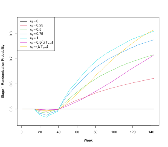
Figure 2: Monte Carlo average randomization probabilities over the course of the trial to the stage 1 option associated with the optimal regime for Scenario 3 under each randomization scheme.

Table 4 summarizes post-trial inference results. For each scenario, the Monte Carlo averages of estimates of $\mu_{s}(a^{opt}_{1,s},a^{opt}_{2,s})$ across the 5000 trials obtained using each of $\widehat{\mu}_{s,Bayes}(a_{1},a_{2})$, $\widehat{\mu}_{s,samp}(a_{1},a_{2})$, and $\widehat{\mu}_{s,wtsamp}(a_{1},a_{2})$ are presented; in all cases, the Bayesian estimator $\widehat{\mu}_{s,Bayes}(a_{1},a_{2})$ was calculated using $M=1000$. Also shown for each estimator are Monte Carlo coverage of a 95% Wald confidence interval for $\mu_{s}(a^{opt}_{1,s},a^{opt}_{2,s})$ and the Monte Carlo proportion of trials in which each estimator correctly identifies the optimal regime. For $\widehat{\mu}_{s,samp}(a_{1},a_{2})$ and $\widehat{\mu}_{s,wtsamp}(a_{1},a_{2})$, Monte Carlo efficiency of these estimators relative to $\widehat{\mu}_{s,Bayes}(a_{1},a_{2})$, defined as the Monte Carlo mean square error for $\widehat{\mu}_{s,Bayes}(a_{1},a_{2})$ divided by that for the given estimator, is presented.

Table 4: Post-trial results, $n_{s}=200$. For each estimator, Est pCR Rate Opt Regime is the Monte Carlo average of estimates of the value of the optimal regime; Coverage is the Monte Carlo coverage of a nominal 95% Wald confidence interval for $\mu_{s}(a^{opt}_{1,s},a^{opt}_{2,s})$; Prop Est Correct is the Monte Carlo proportion of trials for which the true optimal regime was correctly identified as optimal; and Rel Efficiency is the Monte Carlo relative efficiency of the indicated estimator to $\mu_{s,Bayes}(a_{1},a_{2})$.

Estimator	Measure	SR	TS(0.25)	TS(0.5)	TS(0.75)	TS(1)	TS($0.5t/T_{end}$)	TS($t/T_{end}$)
		Scenario 1, $\mu_{s}(a^{opt}_{1,s},a^{opt}_{2,s})$ = 0.660
$\mu_{s,Bayes}(a_{1},a_{2})$	Est pCR Rate Opt Regime	0.640	0.636	0.631	0.628	0.626	0.635	0.629
	Coverage	0.953	0.949	0.942	0.937	0.923	0.936	0.935
	Prop Est Correct	0.487	0.501	0.507	0.514	0.524	0.517	0.522
$\mu_{s,samp}(a_{1},a_{2})$	Est pCR Rate Opt Regime	0.659	0.651	0.644	0.639	0.635	0.649	0.640
	Coverage	0.939	0.939	0.937	0.929	0.927	0.935	0.933
	Prop Est Correct	0.483	0.502	0.506	0.511	0.518	0.519	0.519
	Rel Efficiency	0.825	0.898	0.906	0.884	0.861	0.902	0.891
$\mu_{s,wtsamp}(a_{1},a_{2})$	Est pCR Rate Opt Regime	–	0.656	0.651	0.648	0.646	0.655	0.649
	Coverage	–	0.940	0.939	0.934	0.931	0.934	0.935
	Prop Est Correct	–	0.502	0.506	0.511	0.518	0.519	0.519
	Rel Efficiency	–	0.921	0.969	0.960	0.949	0.933	0.968
		Scenario 2, $\mu_{s}(a^{opt}_{1,s},a^{opt}_{2,s})$ = 0.712
$\mu_{s,Bayes}(a_{1},a_{2})$	Est pCR Rate Opt Regime	0.685	0.683	0.682	0.681	0.677	0.682	0.680
	Coverage	0.953	0.951	0.938	0.930	0.922	0.946	0.930
	Prop Est Correct	0.725	0.757	0.769	0.789	0.782	0.756	0.776
$\mu_{s,samp}(a_{1},a_{2})$	Est pCR Rate Opt Regime	0.713	0.704	0.700	0.698	0.692	0.702	0.697
	Coverage	0.923	0.943	0.939	0.938	0.930	0.943	0.936
	Prop Est Correct	0.723	0.756	0.769	0.789	0.777	0.759	0.773
	Rel Efficiency	0.898	1.038	1.060	1.038	1.003	1.056	1.066
$\mu_{s,wtsamp}(a_{1},a_{2})$	Est pCR Rate Opt Regime	–	0.708	0.706	0.704	0.701	0.707	0.703
	Coverage	–	0.938	0.939	0.941	0.942	0.939	0.941
	Prop Est Correct	–	0.756	0.769	0.789	0.777	0.759	0.773
	Rel Efficiency	–	1.061	1.139	1.147	1.153	1.105	1.162
		Scenario 3, $\mu_{s}(a^{opt}_{1,s},a^{opt}_{2,s})$ = 0.712
$\mu_{s,Bayes}(a_{1},a_{2})$	Est pCR Rate Opt Regime	0.684	0.681	0.682	0.676	0.675	0.681	0.679
	Coverage	0.949	0.939	0.946	0.926	0.923	0.941	0.929
	Prop Est Correct	0.635	0.662	0.692	0.684	0.684	0.670	0.684
$\mu_{s,samp}(a_{1},a_{2})$	Est pCR Rate Opt Regime	0.712	0.704	0.701	0.692	0.690	0.702	0.696
	Coverage	0.930	0.937	0.945	0.935	0.931	0.943	0.933
	Prop Est Correct	0.648	0.668	0.694	0.688	0.684	0.678	0.694
	Rel Efficiency	0.913	1.028	1.069	1.013	1.006	1.059	1.047
$\mu_{s,wtsamp}(a_{1},a_{2})$	Est pCR Rate Opt Regime	–	0.707	0.707	0.701	0.700	0.707	0.704
	Coverage	–	0.936	0.943	0.941	0.937	0.939	0.935
	Prop Est Correct	–	0.668	0.694	0.688	0.684	0.678	0.694
	Rel Efficiency	–	1.059	1.144	1.135	1.136	1.112	1.146
		Scenario 4, $\mu_{s}(a^{opt}_{1,s},a^{opt}_{2,s})$ = 0.712
$\mu_{s,Bayes}(a_{1},a_{2})$	Est pCR Rate Opt Regime	0.682	0.682	0.679	0.678	0.675	0.681	0.679
	Coverage	0.946	0.944	0.930	0.932	0.921	0.942	0.932
	Prop Est Correct	0.695	0.737	0.741	0.769	0.759	0.741	0.756
$\mu_{s,samp}(a_{1},a_{2})$	Est pCR Rate Opt Regime	0.710	0.704	0.698	0.695	0.691	0.701	0.696
	Coverage	0.928	0.941	0.935	0.935	0.933	0.938	0.943
	Prop Est Correct	0.704	0.743	0.749	0.774	0.765	0.747	0.759
	Rel Efficiency	0.931	1.047	1.061	1.032	0.978	1.055	1.088
$\mu_{s,wtsamp}(a_{1},a_{2})$	Est pCR Rate Opt Regime	–	0.708	0.703	0.703	0.700	0.706	0.703
	Coverage	–	0.940	0.938	0.937	0.936	0.936	0.946
	Prop Est Correct	–	0.743	0.749	0.774	0.765	0.745	0.759
	Rel Efficiency	–	1.075	1.141	1.161	1.109	1.097	1.202

All estimators exhibit some downward bias in estimating the value of the optimal regime under all randomization strategies; the sole exception is $\widehat{\mu}_{s,samp}(a_{1},a_{2})$ under SR, where standard asymptotic theory holds. The weighted estimator $\widehat{\mu}_{s,wtsamp}(a_{1},a_{2})$ shows the smallest bias overall. Monte Carlo coverage probabilities of confidence intervals in most cases are close to or slightly less than the nominal 0.95 level, which is likely in part a sample size issue. Lower coverage in many cases tends to be associated with more aggressive adaptive randomization, although this is not uniformly true. Overall, the length of confidence intervals based on $\widehat{\mu}_{s,Bayes}(a_{1},a_{2})$ is slightly less than that of those based on the frequentist estimators (not shown for brevity). Under Scenarios 2-4, involving delayed effects, the weighted estimator is most efficient for estimating the value of the optimal regime and achieves only slightly less precision than that of $\widehat{\mu}_{s,Bayes}(a_{1},a_{2})$ under Scenario 1, with no delayed effects. Under all scenarios, with SR, not surprisingly, the Bayesian estimator yields improved precision over the plug-in sample proportion estimator.

Figure 3 presents histograms of the 5000 estimates of $\mu_{s}(a^{opt}_{1,s},a^{opt}_{2,s})$ in Scenario 3 with TS(1) adaptive randomization using all three estimators, centered by the true value and scaled by standard error; ideally, these quantities should be approximately standard normal. Consistent with the findings of Zhang et al. (2021)²⁶ and Norwood et al. (2024)¹⁷ and with the bias noted above, the distributions of $\widehat{\mu}_{s,Bayes}(a_{1},a_{2})$ and $\widehat{\mu}_{s,samp}(a_{1},a_{2})$ are centered below zero, the latter reflecting the failure of standard asymptotic theory under adaptive randomization. The histogram for $\widehat{\mu}_{s,wtsamp}(a_{1},a_{2})$ is centered at zero, confirming that asymptotic normality is achieved through the weighting. Fortunately, the effects of this behavior on confidence interval performance for the three estimators are unremarkable. Finally, in all of Scenarios 1-4, the proportion of trials in which each estimator identifies the optimal regime is increased under adaptive randomization relative to SR, with the rate of correct identification increasing with the aggressiveness of adaptive randomization.

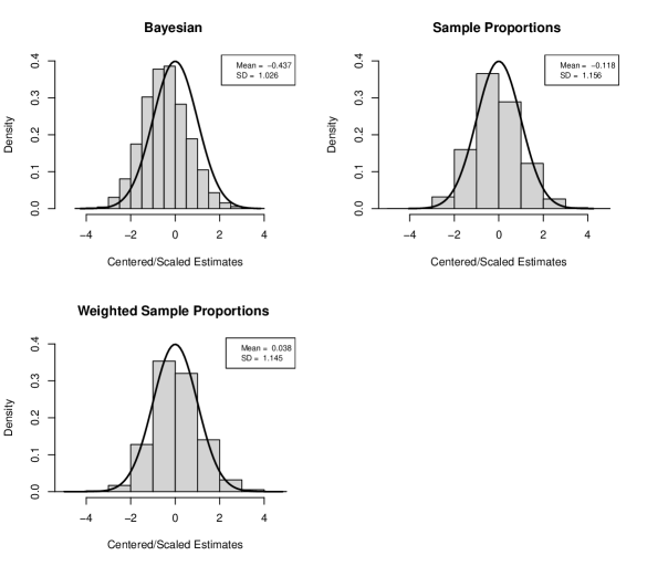
Figure 3: Histograms of 5000 centered and scaled estimates of $\mu_{s}(a^{opt}_{1,s},a^{opt}_{2,s})$ for Scenario 3 under TS(1) adaptive randomization using the Bayesian estimator $\widehat{\mu}_{s,Bayes}(a_{1},a_{2})$, estimator based on sample proportions $\widehat{\mu}_{s,samp}(a_{1},a_{2})$, and estimator based on weighted sample proportions $\widehat{\mu}_{s,wtsamp}(a_{1},a_{2})$.

As noted in Section 1, a concern in conventional RCTs is the potential for loss of efficiency of post-trial inference on treatment effects under adaptive randomization relative to SR. For each estimator and estimation of the value of the optimal regime under each scenario, Table 5 shows Monte Carlo relative efficiency of the indicated estimator under each adaptive randomization scheme to the estimator under SR; because the natural frequentist estimator under SR is $\widehat{\mu}_{s,samp}(a_{1},a_{2})$, the efficiency shown for $\widehat{\mu}_{s,wtsamp}(a_{1},a_{2})$ under adaptive randomization is relative to $\widehat{\mu}_{s,samp}(a_{1},a_{2})$ under SR. Notably, the weighted estimator under adaptive randomization is relatively more efficient in most cases, with mild to moderate efficiency loss only under the most aggressive schemes. Efficiency of $\widehat{\mu}_{s,samp}(a_{1},a_{2})$ under adaptive randomization relative to that under SR shows a similar but less dramatic pattern. The Bayesian estimator $\widehat{\mu}_{s,Bayes}(a_{1},a_{2})$ shows only modest gains or losses under less aggressive adaptation and greater losses than the other two estimators under more aggressive adaptation, possibly a consequence of its larger bias. Overall, the results suggest that all estimators perform well under less aggressive schemes, with $\widehat{\mu}_{s,wtsamp}(a_{1},a_{2})$ gaining efficiency relative to estimation under SR under these conditions, with no or only modest losses under scenarios involving delayed effects.

Table 5: Post-trial results, $n_{s}=200$. For each estimator for the optimal regime for each scenario, Monte Carlo relative efficiency of the estimator under adaptive randomization to the estimator under SR (Monte Carlo mean square error of the estimator under SR divided by that under the indicated adaptive randomization scheme). For $\mu_{s,wtsamp}(a_{1},a_{2})$, efficiency is relative to $\mu_{s,samp}(a_{1},a_{2})$ under SR.

Scenario	Estimator	TS(0.25)	TS(0.5)	TS(0.75)	TS(1)	TS($0.5t/T_{end}$)	TS($t/T_{end}$)
1	$\mu_{s,Bayes}(a_{1},a_{2})$	0.962	0.868	0.800	0.733	0.930	0.831
	$\mu_{s,samp}(a_{1},a_{2})$	1.047	0.953	0.857	0.765	1.017	0.897
	$\mu_{s,wtsamp}(a_{1},a_{2})$	1.075	1.020	0.931	0.844	1.051	0.975
2	$\mu_{s,Bayes}(a_{1},a_{2})$	1.051	0.997	0.934	0.820	1.034	0.935
	$\mu_{s,samp}(a_{1},a_{2})$	1.215	1.178	1.080	0.917	1.216	1.110
	$\mu_{s,wtsamp}(a_{1},a_{2})$	1.242	1.266	1.194	1.054	1.272	1.211
3	$\mu_{s,Bayes}(a_{1},a_{2})$	0.962	1.011	0.802	0.749	0.973	0.872
	$\mu_{s,samp}(a_{1},a_{2})$	1.083	1.184	0.890	0.825	1.128	1.000
	$\mu_{s,wtsamp}(a_{1},a_{2})$	1.115	1.266	0.997	0.932	1.184	1.097
4	$\mu_{s,Bayes}(a_{1},a_{2})$	1.050	0.941	0.876	0.776	1.035	0.964
	$\mu_{s,samp}(a_{1},a_{2})$	1.180	1.072	0.972	0.815	1.173	1.126
	$\mu_{s,wtsamp}(a_{1},a_{2})$	1.213	1.153	1.093	0.924	1.220	1.245

The foregoing results demonstrate that adaptive randomization using the proposed approach based on Thompson sampling results in higher proportions of trial participants being exposed to more efficacious treatment strategies and modest improvements in the overall average pCR rate under conditions like those anticipated in the I-SPY2.2 SMART. Adaptive randomization also results in improved ability to identify the optimal regime using any of the estimators post trial. Based on these and other empirical studies we have conducted, with adaptive randomization and under realistic conditions, we conclude that the Bayesian and weighted sample proportion estimators achieve reliable estimation performance.

In all of Scenarios 1-4, reflecting expectations of the investigators, there is a unique optimal regime among the six embedded regimes, with some of the regimes achieving similar pCR rates/values. To gain insight into performance when there is not a unique optimal regime, in the Appendix we consider an extreme “null” scenario in which all regimes achieve the same pCR rate. Under these conditions, there is no affect of adaptative randomization on in-trial results, as expected. For post-trial inference, all estimators show downward bias; however, the Bayesian estimator achieves the best performance in terms of confidence interval coverage and efficiency relative to $\widehat{\mu}_{s,samp}(a_{1},a_{2})$ and $\widehat{\mu}_{s,wtsamp}(a_{1},a_{2})$ under all randomization schemes. Moreover, efficiency of $\widehat{\mu}_{s,Bayes}(a_{1},a_{2})$ under adaptive randomization relative to SR is markedly better than that for the other two estimators. Although limited, these results support the use of $\widehat{\mu}_{s,Bayes}(a_{1},a_{2})$ for post-trial inference when several regimes are expected to be optimal or close to optimal.

5 Discussion

We have reported on the Bayesian response-adaptive randomization strategy we developed for use in the I-SPY2.2 SMART, which is being implemented in the ongoing trial. The proposed scheme is based on variants of Thompson sampling and exploits the structure of the design to yield straightforward implementation. The formulation also suggests Bayesian and frequentist estimators for subtype-specific pCR rates associated with the regimes embedded in the trial that can be used for post-trial inference on regimes and for identifying the optimal regime. Use of the approach results in higher proportions of participants being randomized to optimal regimes and to modestly higher in-trial overall pCR rates. The strategy was developed specifically for I-SPY2.2, so the evaluation of performance reported here is under conditions similar to those expected in this trial and suggests that the use of adaptive randomization will achieve the investigators’ objectives of assigning more trial participants to more efficacious regimes, resulting in improved outcomes, while not compromising the quality of evenutal post-trial inference for identifying the most efficacious treatment strategies. The form of the true value of an embedded regime in (15) aligns with the intuition that screening patients for achievement of pCR using an algorithm with high specificity, which will identify patients who have not reached pCR with high probability and advance them to further treatment rather than performing surgery too early, will yield more efficacious strategies.

The general approach to adaptive randomization based on Bayesian implementation of the g-computation algorithm and Thompson sampling that we have developed for I-SPY2.2 can be translated straightforwardly to other SMART settings, as can the associated estimators for the values of the embedded regimes.

*Acknowledgments This research is supported by the National Cancer Institute of the National Institutes of Health through grants P01CA210961 (CY, DW, MD) and R01CA280970 (MD).

Appendix A Formulation of value estimators

For convenience, we repeat the following definitions from the main paper. For subtype $s$ and $a_{1}\in\mathcal{A}_{1s}$ and $a_{2}\in\mathcal{A}_{2s}$,

$$\theta_{1}(a_{1})=P(R_{1}=1\mid S=s,A_{1}=a_{1}),\hskip 7.22743pt\gamma_{1}(a_{1})=P(Y_{1}=1\mid S=s,A_{1}=a_{1},R_{1}=1),$$ (A1)

$$\theta_{2}(a_{1},a_{2})=P(R_{2}=1\mid S=s,A_{1}=a_{1},R_{1}=0,A_{2}=a_{2}),\hskip 5.05942pt\gamma_{2}(a_{1},a_{2})=P(Y_{2}=1\mid S=s,A_{1}=a_{1},R_{1}=0,A_{2}=a_{2},R_{2}=1).$$ (A2)

and

$$\gamma_{3,s}(a_{1},a_{2})=P(Y_{3}=1\mid S=s,A_{1}=a_{1},R_{1}=0,A_{2}=a_{2},R_{2}=0).$$ (A3)

Then the value of the subtype $s$-specific regime $\{a_{1},a_{2}\}$, i.e., the probability of achieving pCR if the population of subjects of subtype $s$ were to follow regime $\{a_{1},a_{2}\}$, is

$$\mu_{s}(a_{1},a_{2}) =\theta_{1}(a_{1})\gamma_{1}(a_{1})+\{1-\theta_{1}(a_{1})\}\theta_{2}(a_{1},a_{2})\gamma_{2}(a_{1},a_{2})$$ (A4)

$$+\{1-\theta_{1}(a_{1})\}\{1-\theta_{2}(a_{1},a_{2})\}\gamma_{3,s}(a_{1},a_{2}).$$

Suppose that there are $n$ subjects across all subtypes, $n_{s}$ of whom are from of subtype $s$. Note that at any week $t$, as seen in Table 1 in the main paper, the part of the available data $\mathcal{D}_{t}$ on previously enrolled subjects that are relevant to updating randomization probabilities for subjects of subtype $s$ at week $t$ are the subsets of $\mathcal{O}$ that have already been observed before $t$ on among the $n_{s}$ subjects who enrolled prior to $t$. Indexing these $n_{s}$ subjects by $i$, at the conclusion of the trial, the part of the final data $\mathcal{D}_{final}$ relevant to estimating $\mu_{s}(a_{1},a_{2})$ for subtype $s$ are $\mathcal{O}_{i}$, $i=1,\ldots,n_{s}$. As discussed in the main paper, the proposed Bayesian estimator $\widehat{\mu}_{s,Bayes}(a_{1},a_{2})$ is calculated based on these data. Namely, with

$$\Theta_{1,s}=\{\gamma_{1,s}(a_{1}),\gamma_{2,s}(a_{1},a_{2}),\gamma_{3,s}(a_{1},a_{2}),\theta_{1,s}(a_{1}),\theta_{2,s}(a_{1},a_{2});\,\,\,(a_{1},a_{2})\in\mathcal{A}_{1,s}\times\mathcal{A}_{2,s}\},$$

to estimate the value of the subtype $s$-specific embedded regime $\{a_{1},a_{2}\}$, draw a sample of size $M$ from each of the posterior distributions given $\mathcal{D}_{final}$ of the components of $\Theta_{1,s}$ to obtain draws $\Theta_{1,s}^{(m)}$, $m=1,\ldots,M$, from the joint posterior of $\Theta_{1,s}$ given $\mathcal{D}_{final}$. Then substitute each of these draws in (A4) to obtain $\mu^{(m)}_{s}(a_{1},a_{2})$, $m=1,\ldots,M$, which can be viewed as a sample from the posterior distribution of $\mu_{s}(a_{1},a_{2})$ given $\mathcal{D}_{final}$. The Bayesian estimator $\widehat{\mu}_{s,Bayes}(a_{1},a_{2})$ is obtained as the mean or mode of the sample, with the standard deviation of the sample as a measure of uncertainty.

We now present the formulation of the alternative estimators $\widehat{\mu}_{s,samp}(a_{1},a_{2})$ and $\widehat{\mu}_{s,wtsamp}(a_{1},a_{2})$ based on the final data $\mathcal{O}_{i}$, $i=1,\ldots,n_{s}$ on the subjects of subtype $s$. These estimators may have appeal in that they can be considered as frequentist alternatives to $\widehat{\mu}_{s,Bayes}(a_{1},a_{2})$. First, note from (A1)-(A3) that

$$\theta_{1}(a_{1})\gamma_{1}(a_{1})=\frac{\alpha_{1,s}(a_{1})}{\alpha_{2,s}(a_{1})}=\frac{P(S=s,A_{1}=a_{1},R_{1}=1,Y_{1}=1)}{P(S=s,A_{1}=a_{1})},$$

$$\theta_{2}(a_{1},a_{2})\gamma_{2}(a_{1},a_{2})=\frac{\alpha_{3,s}(a_{1},a_{2})}{\alpha_{4,s}(a_{1},a_{2})}=\frac{P(S=s,A_{1}=a_{1},R_{1}=0,A_{2}=a_{2},R_{2}=1,Y_{2}=1)}{P(S=s,A_{1}=a_{1},R_{1}=0,A_{2}=a_{2})},$$

$$\{1-\theta_{2}(a_{1},a_{2})\}\gamma_{2}(a_{1},a_{2})=\frac{\alpha_{5,s}(a_{1},a_{2})}{\alpha_{4,s}(a_{1},a_{2})}=\frac{P(S=s,A_{1}=a_{1},R_{1}=0,A_{2}=a_{2},R_{2}=0,Y_{3}=1)}{P(S=s,A_{1}=a_{1},R_{1}=0,A_{2}=a_{2})},$$

$$\{1-\theta_{1}(a_{1})\}=\frac{\alpha_{6,s}(a_{1})}{\alpha_{2,s}(a_{1})}=\frac{P(S=s,A_{1}=a_{1},R_{1}=0)}{P(S=s,A_{1}=a_{1})}.$$

Thus, $\mu_{s}(a_{1},a_{2})$ also can be written as

$$\mu_{s}(a_{1},a_{2})=\frac{\alpha_{1}(a_{1,s})}{\alpha_{2,s}(a_{1})}+\frac{\alpha_{6,s}(a_{1})}{\alpha_{2,s}(a_{1})}\left\{\frac{\alpha_{3,s}(a_{1},a_{2})+\alpha_{5,s}(a_{1},a_{2})}{\alpha_{4,s}(a_{1},a_{2})}\right\}.$$ (A5)

Given the representation in (A5), a natural plug-in estimator is based on substituting sample proportions for the probabilities $\alpha_{1,s}(a_{1}),\alpha_{2,s}(a_{1}),\alpha_{3,s}(a_{1},a_{2}),\alpha_{4,s}(a_{1},a_{2}),\alpha_{5,s}(a_{1},a_{2}),\alpha_{6,s}(a_{1})$, namely,

$$\widehat{\mu}_{s,samp}(a_{1},a_{2})=\frac{\widehat{\alpha}_{1,s}(a_{1})}{\widehat{\alpha}_{2,s}(a_{1})}+\frac{\widehat{\alpha}_{6,s}(a_{1})}{\widehat{\alpha}_{2,s}(a_{1})}\left\{\frac{\widehat{\alpha}_{3,s}(a_{1},a_{2})+\widehat{\alpha}_{5,s}(a_{1},a_{2})}{\widehat{\alpha}_{4,s}(a_{1},a_{2})}\right\},$$ (A6)

where

$$\widehat{\alpha}_{1,s}(a_{1})=n^{-1}_{s}\sum_{i=1}^{n_{s}}I(A_{1i}=a_{1},R_{1i}=1,Y_{1i}=1),\hskip 7.22743pt\widehat{\alpha}_{2,s}(a_{1})=n^{-1}_{s}\sum_{i=1}^{n_{s}}I(A_{1i}=a_{1}),$$

$$\widehat{\alpha}_{3,s}(a_{1},a_{2})=n^{-1}_{s}\sum_{i=1}^{n_{s}}I(A_{1i}=a_{1},R_{1i}=0,A_{2i}=a_{2},R_{2i}=1,Y_{2i}=1),\hskip 7.22743pt\widehat{\alpha}_{4,s}(a_{1},a_{2})=n^{-1}_{s}\sum_{i=1}^{n_{s}}I(A_{1i}=a_{1},R_{1i}=0,A_{2i}=a_{2}),$$

$$\widehat{\alpha}_{5,s}(a_{1},a_{2})=n^{-1}_{s}\sum_{i=1}^{n_{s}}I(A_{1i}=a_{1},R_{1i}=0,A_{2i}=a_{2},R_{2i}=0,Y_{3i}=1),\hskip 7.22743pt\widehat{\alpha}_{6,s}(a_{1})=n^{-1}_{s}\sum_{i=1}^{n_{s}}I(A_{1i}=a_{1},R_{1i}=0).$$

Note that in these expressions we do not include $S_{i}=s$ in the indicator functions, as the sums are over only subjects $i$ for whom $S_{i}=s$ is true.

As discussed in Section 3.3 of the main paper, because of the use of adaptive randomization, the final data from subjects of subtype $s$, $\mathcal{O}_{i}$, $i=1,\ldots,n_{s}$, are not independent and identically distributed (i.i.d.) over $i$, so that standard asymptotic theory may not apply to derive the properties of (A6). Thus, it is not even clear that the estimators above are consistent estimators for the corresponding probabilities. Nonetheless, proceeding naively as if the data are i.i.d. and applying standard theory, one can derive an approximate standard error for $\widehat{\mu}_{s,samp}(a_{1},a_{2})$ by finding the associated influence function. We provide a heuristic argument. Denote by $\alpha^{*}_{1,s}(a_{1}),\alpha^{*}_{2,s}(a_{1}),\alpha^{*}_{3,s}(a_{1},a_{2}),\alpha^{*}_{4,s}(a_{1},a_{2}),\alpha^{*}_{5,s}(a_{1},a_{2}),\alpha^{*}_{6,s}(a_{1})$ the limits in probability of $\widehat{\alpha}_{1}(a_{1}),\widehat{\alpha}_{2}(a_{1}),\widehat{\alpha}_{3,s}(a_{1},a_{2}),\widehat{\alpha}_{4,s}(a_{1},a_{2}),\widehat{\alpha}_{5,s}(a_{1},a_{2}),\widehat{\alpha}_{6,s}(a_{1})$, which would be the corresponding true probabilities if the data were i.i.d. Let

$$\mu^{*}_{s}(a_{1},a_{2})=\frac{\alpha^{*}_{1,s}(a_{1})}{\alpha^{*}_{2,s}(a_{1})}+\frac{\alpha^{*}_{6,s}(a_{1})}{\alpha^{*}_{2,s}(a_{1})}\left\{\frac{\alpha^{*}_{3,s}(a_{1},a_{2})+\alpha^{*}_{5,s}(a_{1},a_{2})}{\alpha^{*}_{4,s}(a_{1},a_{2})}\right\}.$$

We find the mean-zero quantity $\mathcal{I}_{i}$ such that

$$n^{1/2}_{s}\left\{\widehat{\mu}_{s}(a_{1},a_{2})-\mu^{*}_{s}(a_{1},a_{2})\right\}=n^{-1/2}_{s}\sum_{i=1}^{n_{s}}\mathcal{I}_{i}+o_{p}(1).$$ (A7)

As is well known, with i.i.d. data, it follows that the left hand side of (A7) converges in distribution to a normal random variable with mean zero and variance that can be approximated by $n^{-1}_{s}\sum_{i=1}^{n_{s}}\mathcal{I}_{i}^{2}$. Assuming that $n^{1/2}_{s}\{\widehat{\alpha}_{j,s}(a_{1})-\alpha^{*}_{j,s}(a_{1})\}=O_{p}(1)$, $j=1,2,6$, and $n^{1/2}_{s}\{\widehat{\alpha}_{j,s}(a_{1},a_{2})-\alpha^{*}_{j,s}(a_{1},a_{2})\}=O_{p}(1)$, $j=3,4,5$, so are bounded in probability, it is straightforward by tedious algebra to show that

$$n^{1/2}_{s} \left\{\widehat{\mu}_{s,samp}(a_{1},a_{2})-\mu^{*}_{s}(a_{1},a_{2})\right\}=\left\{\frac{1}{\alpha^{*}_{2,s}(a_{1})}\right\}\left(n^{1/2}_{s}\{\widehat{\alpha}_{1,s}(a_{1})-\alpha^{*}_{1,s}(a_{1})\}-\mu^{*}_{s}(a_{1},a_{2})\,n^{1/2}_{s}\{\widehat{\alpha}_{2,s}(a_{1})-\alpha^{*}_{2,s}(a_{1})\}\vphantom{\frac{n^{1/2}_{s}(\widehat{\alpha}_{4,s}(a_{1},a_{2})-\alpha^{*}_{4,s}(a_{1},a_{2}))}{\alpha^{*}_{4,s}(a_{1},a_{2})}}\right.$$ (A8)

$$\hskip 3.61371pt+\left\{\frac{\alpha^{*}_{3,s}(a_{1},a_{2})+\alpha^{*}_{5,s}(a_{1},a_{2})}{\alpha^{*}_{4,s}(a_{1},a_{2})}\right\}\left[-\left\{\frac{\alpha^{*}_{6,s}(a_{1})}{\alpha^{*}_{4,s}(a_{1},a_{2})}\right\}n^{1/2}_{s}\{\widehat{\alpha}_{4,s}(a_{1},a_{2})-\alpha^{*}_{4,s}(a_{1},a_{2})\}+n^{1/2}_{s}\{\widehat{\alpha}_{6,s}(a_{1})-\alpha^{*}_{6,s}(a_{1})\}\right]$$

$$\hskip 3.61371pt+\left\{\frac{\alpha^{*}_{6,s}(a_{1})}{\alpha^{*}_{4,s}(a_{1},a_{2})}\right\}n^{1/2}_{s}\left[\{\widehat{\alpha}_{3,s}(a_{1},a_{2})+\widehat{\alpha}_{5,s}(a_{1},a_{2})\}-\{\alpha^{*}_{3,s}(a_{1},a_{2})+\alpha^{*}_{5,s}(a_{1},a_{2})\}\right]\left.\vphantom{\frac{n^{1/2}_{s}(\widehat{\alpha}_{4,s}(a_{1},a_{2})-\alpha^{*}_{4,s}(a_{1},a_{2}))}{\alpha^{*}_{4,s}(a_{1},a_{2})}}\right)+o_{p}(1).$$

Substituting the expressions for $\widehat{\alpha}_{1,s}(a_{1}),\widehat{\alpha}_{2,s}(a_{1}),\widehat{\alpha}_{3,s}(a_{1},a_{2}),\widehat{\alpha}_{4,s}(a_{1},a_{2}),\widehat{\alpha}_{5,s}(a_{1},a_{2}),\widehat{\alpha}_{6,s}(a_{1})$ in (A8) and simplifying leads to

$$\mathcal{I}_{i} =\left\{\frac{1}{\alpha^{*}_{2,s}(a_{1})}\right\}\left(I(A_{1i}=a_{1},R_{1i}=1,Y_{1i}=1)-\alpha^{*}_{1,s}(a_{1})-\mu^{*}_{s}(a_{1},a_{2})\{I(A_{1i}=a_{1})-\alpha^{*}_{2,s}(a_{1})\}\vphantom{\left(\frac{\alpha^{*}_{3,s}(a_{1},a_{2})+\alpha^{*}_{5,s}(a_{1},a_{2})}{\alpha^{*}_{4,s}(a_{1},a_{2})}\right)}\right.$$

$$\hskip 3.61371pt+\left\{\frac{\alpha^{*}_{3,s}(a_{1},a_{2})+\alpha^{*}_{5,s}(a_{1},a_{2})}{\alpha^{*}_{4,s}(a_{1},a_{2})}\right\}\left[-\left\{\frac{\alpha^{*}_{6,s}(a_{1})}{\alpha^{*}_{4,s}(a_{1},a_{2})}\right\}\left\{I(A_{1i}=a_{1},R_{1i}=0,A_{2i}=a_{2})-\alpha^{*}_{4,s}(a_{1},a_{2})\right\}+\left\{I(A_{1i}=a_{1},R_{1i}=0)-\alpha^{*}_{6,s}(a_{1})\right\}\right]$$

$$\hskip 3.61371pt+\left.\left\{\frac{\alpha^{*}_{6,s}(a_{1})}{\alpha^{*}_{4,s}(a_{1},a_{2})}\right\}\left[\vphantom{\{\alpha^{*}_{3,s}(a_{1},a_{2})+\alpha^{*}_{5,s}(a_{1},a_{2}\}}I(A_{1i}=a_{1},R_{1i}=0,A_{2i}=a_{2},R_{2i}=1,Y_{2i}=1)+I(A_{1i}=a_{1},R_{1i}=0,A_{2i}=a_{2},R_{2i}=0,Y_{3i}=1)\right.\right.$$

$$\hskip 61.42993pt\left.\left.-\{\alpha^{*}_{3,s}(a_{1},a_{2})+\alpha^{*}_{5,s}(a_{1},a_{2}\}\vphantom{\left[I(A_{1i}=a_{1},R_{1i}=0,A_{2i}=a_{2},R_{2i}=1,Y_{2i}=1)+I(A_{1i}=a_{1},R_{1i}=0,A_{2i}=a_{2},R_{2i}=0,Y_{3i}=1)\right]}\right]\vphantom{\left\{\frac{\alpha^{*}_{6,s}(a_{1})}{\alpha^{*}_{4,s}(a_{1},a_{2})}\right\}}\right).$$ (A9)

Assuming that $n_{s}^{-1}\sum_{i=1}^{n_{s}}\mathcal{I}_{i}^{2}$ converges in probability to $\Sigma>0$, we can conclude that $n_{s}^{1/2}\left\{\widehat{\mu}_{s,samp}(a_{1},a_{2})-\mu^{*}_{s}(a_{1},a_{2})\right\}$ converges in distribution to a mean-zero normal random variable with variance $\Sigma$.

For practical use, letting $\widehat{\mathcal{I}}_{i}$ denote (A9) with $\widehat{\alpha}_{1,s}(a_{1}),\widehat{\alpha}_{2,s}(a_{1}),\widehat{\alpha}_{3,s}(a_{1},a_{2}),\widehat{\alpha}_{4,s}(a_{1},a_{2}),\widehat{\alpha}_{5,s}(a_{1},a_{2}),\widehat{\alpha}_{6,s}(a_{1})$ and $\widehat{\mu}_{s,samp}(a_{1},a_{2})$ substituted for $\alpha^{*}_{1,s}(a_{1}),\alpha^{*}_{2,s}(a_{1}),\alpha^{*}_{3,s}(a_{1},a_{2}),\alpha^{*}_{4,s}(a_{1},a_{2}),\alpha^{*}_{5,s}(a_{1},a_{2}),\alpha^{*}_{6,s}(a_{1})$ and $\mu^{*}_{s}(a_{1},a_{2})$, estimate $\Sigma$ by $n^{-1}_{s}\sum_{i=1}^{n_{s}}\widehat{\mathcal{I}}_{i}^{2}$.

The foregoing result was derived by taking $\mathcal{O}$, $i=1,\ldots,n_{s}$, to be i.i.d. and applying standard theory. Because these data are not i.i.d. owing to the adaptive randomization, inferences based on this result are likely to be flawed. Accordingly, we now consider derivation of the estimator $\widehat{\mu}_{s,wtsamp}(a_{1},a_{2})$, which, as discussed in Section 3.3 of the main paper, involves weighted versions of estimators for each of the probabilities in (A5). The derivation is heuristic and follows the spirit of arguments in Norwood et al. (2024)¹⁷, which adapts the approach of Zhang et al. (2021)²⁶ on theory for M-estimators based on adaptively collected data.

Define the set of all potential outcomes for a randomly chosen patient in the subtype $s$ population as

$$\mathcal{W}^{*}=\{R_{1}^{*}(a_{1}),Y_{1}^{*}(a_{1}),R_{2}^{*}(a_{1},a_{2}),Y_{2}^{*}(a_{1},a_{2}),Y_{3}^{*}(a_{1},a_{2}),\hskip 3.61371pt\mbox{for all}\hskip 3.61371pt(a_{1},a_{2})\in\mathcal{A}_{1,s}\times\mathcal{A}_{2,s}\}.$$

Here, $R_{1}^{*}(a_{1})$ is the response status and $Y_{1}^{*}(a_{1})$ is the pCR status a patient would achieve if given stage 1 treatment $a_{1}$; $R_{2}^{*}(a_{1},a_{2})$ is the response status a patient would achieve if given stage 1 treatment $a_{1}$ followed by stage 2 treatment $a_{2}$; and $Y_{2}^{*}(a_{1},a_{2})$ is the pCR status a patient would achieve if given stage 1 treatment $a_{1}$ followed by stage 2 treatment $a_{2}$ at the end of stage 2, and $Y_{3}2^{*}(a_{1},a_{2})$ is the pCR status at the end of stage 3. Although the observed data $\mathcal{O}_{i}$, $i=1,\ldots,n_{s}$, are not i.i.d., the potential outcomes $\mathcal{W}^{*}_{i}$, $i=1,\ldots,n_{s}$, are i.i.d. We make standard identifiability assumptions, which are discussed extensively elsewhere¹¹: (i) consistency, which implies that observed variables are equal to their potential counterparts under the treatments actually received; (ii) positivity, which implies that the probabilities of being assigned any treatment in $\mathcal{A}_{1,s}$ and $\mathcal{A}_{2,s}$ are strictly greater than zero, which holds in ISPY2.2 through the use of “clipping constants” that prevent adaptive probabilities from dropping below a set threshold; and (iii) sequential randomization, which holds by design in a nonadaptively randomized SMART and is discussed further below in the case the adaptively randomized ISPY2.2 SMART.

From (A5), we can write

$$\mu_{s}(a_{1},a_{2})=\phi_{1,s}(a_{1})+\phi_{2,s}(a_{1})\{\phi_{3,s}(a_{1},a_{2})+\phi_{4,s}(a_{1},a_{2})\},$$ (A10)

where

$$\phi_{1,s}(a_{1}) =\frac{\alpha_{1}(a_{1,s})}{\alpha_{2,s}(a_{1}}=P(R_{1}=1,Y_{1}=1\mid S=s,A_{1}=a_{1})$$ (A11)

$$\phi_{2,s}(a_{1}) =\frac{\alpha_{6,s}(a_{1})}{\alpha_{2}(a_{1})}=P(R_{1}=0\mid S=s,A_{1}=a_{1})$$ (A12)

$$\phi_{3,s}(a_{1},a_{2}) =\frac{\alpha_{3,s}(a_{1},a_{2})}{\alpha_{4,s}(a_{1},a_{2})}=P(R_{2}=1,Y_{2}=1\mid S=s,A_{1}=a_{1},R_{1}=0,A_{2}=a_{2})$$ (A13)

$$\phi_{4,s}(a_{1},a_{2}) =\frac{\alpha_{5,s}(a_{1},a_{2})}{\alpha_{4,s}(a_{1},a_{2})}=P(R_{2}=0,Y_{3}=1\mid S=s,A_{1}=a_{1},R_{1}=0,A_{2}=a_{2})$$ (A14)

For some set of weights $w^{(1)}_{i}(a_{1})$, $i=1,\ldots,n_{s}$, where we reiterate that $i$ indexes only subjects with $S=s$, define

$$\widehat{\alpha}^{w}_{1,s}(a_{1})=n^{-1}_{s}\sum_{i=1}^{n_{s}}w^{(1)}_{i}(a_{1})I(A_{1i}=a_{1},R_{1i}=1,Y_{1i}=1),\hskip 36.8573pt\widehat{\alpha}^{w}_{2,s}(a_{1})=n^{-1}_{s}\sum_{i=1}^{n_{s}}w^{(1)}_{i}(a_{1})I(A_{1i}=a_{1}).$$

Then note that the obvious estimator for $\phi_{1,s}(a_{1})$ in (A11) is $\widehat{\phi}_{1,s}(a_{1})=\widehat{\alpha}^{w}_{1,s}(a_{1})/\widehat{\alpha}^{w}_{2,s}(a_{1})$, which solves in $\phi_{1,s}(a_{1})$ an M-estimating equation of the form

$$\sum_{i=1}^{n_{s}}w^{(1)}_{i}(a_{1})I(A_{1i}=a_{1})\{I(R_{1i}=1,Y_{1i}=1)-\phi_{1,s}(a_{1})\}=\sum_{i=1}^{n_{s}}M\{A_{1i},R_{1i},Y_{1i},a_{1};\phi_{1,s}(a_{1})\}=0.$$ (A15)

Following Zhang et al. (2021)²⁶ and Norwood et al. (2024)¹⁷, we choose the $w^{(1)}_{i}(a_{1})$ so that the estimator $\widehat{\phi}_{1,s}(a_{1})$ is consistent for $\phi_{1,s}(a_{1})$ with asymptotic normal theory that can be established via the martingale central limit theorem. Assume for definiteness that subject $i$ enrolled during the interval $[t,t+1)$, so was assigned to stage 1 treatment according to randomization probabilities $\pi_{1,s,t}(a_{1}\mid\mathcal{D}_{t})$, $a_{1}\in\mathcal{A}_{1,s}$, where as in the main paper $\mathcal{D}_{t}$ comprises the data from subjects enrolling prior to week $t$, and we suppress the damping constant for brevity. Application of the martingale central limit theorem requires that the $w^{(1)}_{i}(a_{1})$, which depend only on $\mathcal{D}_{t}$ and not on data on subject $i$, are chosen so that (i) the estimating equation (A15) remains conditionally (on $\mathcal{D}_{t}$) unbiased, $E[M\{A_{1i},R_{1i},Y_{1i},a_{1};\phi_{1,s}(a_{1})\}\mid\mathcal{D}_{t}]=0$; and (ii) the variance is stabilized, $E[M^{2}\{A_{1i},R_{1i},Y_{1i},a_{1};\phi_{1,s}(a_{1})\}\mid\mathcal{D}_{t}]=\sigma^{2}>0$, a constant not depending on $t$. With $w^{(1)}_{i}(a_{1})$ so chosen, it then follows that the large sample distribution of $\widehat{\phi}_{1,s}(a_{1})$ can approximated as described below.

To show (i), note by the consistency assumption that a summand in (A15) can be written equivalently as

$$w^{(1)}_{i}(a_{1})I(A_{1i}=a_{1})[I\{R_{1i}^{*}(a_{1})=1,Y_{1i}^{*}(a_{1})=1\}-\phi_{1,s}(a_{1})].$$

Note then that

$$E \left(w^{(1)}_{i}(a_{1})I(A_{1i}=a_{1})[I\{R_{1i}^{*}(a_{1})=1,Y_{1i}^{*}(a_{1})=1\}-\phi_{1,s}(a_{1})]\left|\vphantom{E[w^{(1)}_{i}(a_{1})]}\right.\mathcal{D}_{t}\right)$$

$$=E\left\{E\left(w^{(1)}_{i}(a_{1})I(A_{1i}=a_{1})[I\{R_{1i}^{*}(a_{1})=1,Y_{1i}^{*}(a_{1})=1\}-\phi_{1,s}(a_{1})]\left|\vphantom{E[w^{(1)}_{i}(a_{1})]}\right.\mathcal{D}_{t},\mathcal{W}_{i}^{*}\right)\left|\vphantom{E[w^{(1)}_{i}(a_{1})]}\right.\mathcal{D}_{t}\right\}$$

$$=E\left(w^{(1)}_{i}(a_{1})[I\{R_{1i}^{*}(a_{1})=1,Y_{1i}^{*}(a_{1})=1\}-\phi_{1,s}(a_{1})]\,E\{I(A_{1i}=a_{1})\mid\mathcal{D}_{t},\mathcal{W}_{i}^{*}\}\left|\vphantom{E[w^{(1)}_{i}(a_{1})]}\right.\mathcal{D}_{t}\right)$$

$$=w^{(1)}_{i}(a_{1})\pi_{1,s,t}(a_{1}\mid\mathcal{D}_{t})\,E\left([I\{R_{1i}^{*}(a_{1})=1,Y_{1i}^{*}(a_{1})=1\}-\phi_{1,s}(a_{1})]\mid\mathcal{D}_{t}\right)$$ (A16)

$$=w^{(1)}_{i}(a_{1})\pi_{1,s,t}(a_{1}\mid\mathcal{D}_{t})\,E([I\{R_{1i}^{*}(a_{1})=1,Y_{1i}^{*}(a_{1})=1\}-\phi_{1,s}(a_{1})]=0.$$ (A17)

Here, (A16) follows by showing that $E\{I(A_{1i}=a_{1})\mid\mathcal{D}_{t},\mathcal{W}_{i}^{*}\}=\pi_{1,s,t}(a_{1}\mid\mathcal{D}_{t})$ by an argument conditional on $\mathcal{D}_{t}$ similar to that in Section 6.4.3 of Tsiatis et al. (2020)¹¹, noting that $i$ is of subtype $s$. The first equality in (A17) follows because $\mathcal{D}_{t}\mathchoice{\mathrel{\hbox to0.0pt{$\displaystyle\perp$\hss}\mkern 2.0mu{\displaystyle\perp}}}{\mathrel{\hbox to0.0pt{$\textstyle\perp$\hss}\mkern 2.0mu{\textstyle\perp}}}{\mathrel{\hbox to0.0pt{$\scriptstyle\perp$\hss}\mkern 2.0mu{\scriptstyle\perp}}}{\mathrel{\hbox to0.0pt{$\scriptscriptstyle\perp$\hss}\mkern 2.0mu{\scriptscriptstyle\perp}}}\mathcal{W}_{i}^{*}$, where “$\mathchoice{\mathrel{\hbox to0.0pt{$\displaystyle\perp$\hss}\mkern 2.0mu{\displaystyle\perp}}}{\mathrel{\hbox to0.0pt{$\textstyle\perp$\hss}\mkern 2.0mu{\textstyle\perp}}}{\mathrel{\hbox to0.0pt{$\scriptstyle\perp$\hss}\mkern 2.0mu{\scriptstyle\perp}}}{\mathrel{\hbox to0.0pt{$\scriptscriptstyle\perp$\hss}\mkern 2.0mu{\scriptscriptstyle\perp}}}$” denotes “independent of” (i.e., the data from past subjects are independent of the potential outcomes for subject $i$); and the second equality follows because in the ISPY2.2 SMART randomization at the first stage guarantees that $A_{1i}\mathchoice{\mathrel{\hbox to0.0pt{$\displaystyle\perp$\hss}\mkern 2.0mu{\displaystyle\perp}}}{\mathrel{\hbox to0.0pt{$\textstyle\perp$\hss}\mkern 2.0mu{\textstyle\perp}}}{\mathrel{\hbox to0.0pt{$\scriptstyle\perp$\hss}\mkern 2.0mu{\scriptstyle\perp}}}{\mathrel{\hbox to0.0pt{$\scriptscriptstyle\perp$\hss}\mkern 2.0mu{\scriptscriptstyle\perp}}}\mathcal{W}_{i}^{*}$ given that $i$ is of subtype $s$ (as in the sequential randomization assumption). Thus, using the consistency assumption,

$$P\{R_{1i}^{*}(a_{1})=1, Y_{1i}^{*}(a_{1})=1\}=P\{R_{1i}^{*}(a_{1})=1,Y_{1i}^{*}(a_{1})=1\mid A_{1i}=a_{1}\}$$

$$=P(R_{1i}=1,Y_{1i}=1\mid A_{1i}=1)=P(R_{1}=1,Y_{1}=1\mid S=s,A_{1}=a_{1})=\phi_{1,s}(a_{1}),$$

given that $i$ is from subtype $s$. Thus (i) holds for any $w^{(1)}_{i}(a_{1})$ depending only on $\mathcal{D}_{t}$. To determine $w^{(1)}_{i}(a_{1})$ depending on $\mathcal{D}_{t}$ such that (ii) is satisfied, note that, similarly to the above, and using $\{I(A_{1i}=a_{1})\}^{2}=I(A_{1i}=a_{1})$,

$$E \left(\{w^{(1)}_{i}(a_{1})\}^{2}I(A_{1i}=a_{1})[I\{R_{1i}^{*}(a_{1})=1,Y_{1i}^{*}(a_{1})=1\}-\phi_{1,s}(a_{1})]^{2}\left|\vphantom{\{w^{(1)}_{i}(a_{1})\}^{2}}\right.\mathcal{D}_{t}\right)$$

$$=E\left(\{w^{(1)}_{i}(a_{1})\}^{2}[I\{R_{1i}^{*}(a_{1})=1,Y_{1i}^{*}(a_{1})=\}-\phi_{1,s}(a_{1})]^{2}\,E\{I(A_{1i}=a_{1})\mid\mathcal{D}_{t},\mathcal{W}_{i}^{*}\}\left|\vphantom{\{w^{(1)}_{i}(a_{1})\}^{2}}\right.\mathcal{D}_{t}\right)$$

$$=\{w^{(1)}_{i}(a_{1})\}^{2}\pi_{1,s,t}(a_{1}\mid\mathcal{D}_{t})\,E\left([I\{(R_{1i}^{*}(a_{1})=1,Y_{1i}^{*}(a_{1})=1\}-\phi_{1,s}(a_{1})]^{2}\mid\mathcal{D}_{t}\right)$$

$$=\{w^{(1)}_{i}(a_{1})\}^{2}\pi_{1,s,t}(a_{1}\mid\mathcal{D}_{t})\,E\left([I\{R_{1i}^{*}(a_{1})=1,Y_{1i}^{*}(a_{1})1\}-\phi_{1,s}(a_{1})]^{2}\right),$$ (A18)

where (A18) follows because $\mathcal{D}_{t}\mathchoice{\mathrel{\hbox to0.0pt{$\displaystyle\perp$\hss}\mkern 2.0mu{\displaystyle\perp}}}{\mathrel{\hbox to0.0pt{$\textstyle\perp$\hss}\mkern 2.0mu{\textstyle\perp}}}{\mathrel{\hbox to0.0pt{$\scriptstyle\perp$\hss}\mkern 2.0mu{\scriptstyle\perp}}}{\mathrel{\hbox to0.0pt{$\scriptscriptstyle\perp$\hss}\mkern 2.0mu{\scriptscriptstyle\perp}}}\mathcal{W}_{i}^{*}$. Clearly, because the $\mathcal{W}_{i}^{*}$ are i.i.d., $E\left([I\{R_{1i}^{*}(a_{1})=1,Y_{1i}^{*}(a_{1})=1\}-\phi_{1,s}(a_{1})]^{2}\right)$ is the same constant for any $i$ (and thus $t$). Thus, the entire expression in (A18) will be a constant not depending on $t$ if we take

$$w^{(1)}_{i}(a_{1})=1/\sqrt{\pi_{1,s,t}(a_{1}\mid\mathcal{D}_{t})}.$$ (A19)

An entirely similar argument can be made for estimation of $\phi_{2,s}(a_{1})$. Namely, letting

$$\widehat{\alpha}^{w}_{6,s}(a_{1})=n^{-1}_{s}\sum_{i=1}^{n_{s}}w^{(1)}_{i}(a_{1})I(A_{1i}=a_{1},R_{1i}=0),$$

the estimator $\widehat{\phi}_{2,s}(a_{1})=\widehat{\alpha}^{w}_{6,s}(a_{1})/\widehat{\alpha}^{w}_{2,s}(a_{1})$ for $\phi_{2,s}(a_{1})$ in (A12) solves in $\phi_{2,s}(a_{1})$ an M-estimating equation of the form

$$\sum_{i=1}^{n_{s}}w^{(1)}_{i}(a_{1})I(A_{1i}=a_{1})\{I(R_{1i}=0-\phi_{2,s}(a_{1})\}=\sum_{i=1}^{n_{s}}M\{A_{1i},R_{1i},a_{1};\phi_{2,s}(a_{1})\}=0.$$ (A20)

Arguments analogous to those above show that $w^{(1)}_{i}(a_{1})$ should be chosen as in (A19).

Similar arguments are possible for estimation of $\phi_{3,s}(a_{1},a_{2})$ and $\phi_{4,s}(a_{1},a_{2})$ in (A13) and (A14). For a set of weights $w^{(2)}_{i}(a_{1},a_{2})$, $i=1,\ldots,n_{s}$, define

$$\widehat{\alpha}^{w}_{3,s}(a_{1},a_{2})=n^{-1}_{s}\sum_{i=1}^{n_{s}}w^{(2)}_{i}(a_{1},a_{2})I(A_{1i}=a_{1},R_{1i}=0,A_{2i}=a_{2},R_{2i}=1,Y_{2i}=1),$$

$$\widehat{\alpha}^{w}_{4,s}(a_{1},a_{2})=n^{-1}_{s}\sum_{i=1}^{n_{s}}w^{(2)}_{i}(a_{1},a_{2})I(A_{1i}=a_{1},R_{1i}=0,A_{2i}=a_{2})$$

$$\widehat{\alpha}^{w}_{5,s}(a_{1},a_{2})=n^{-1}_{s}\sum_{i=1}^{n_{s}}w^{(2)}_{i}(a_{1},a_{2})I(A_{1i}=a_{1},R_{1i}=0,A_{2i}=a_{2},R_{2i}=0,Y_{3i}=1).$$

Then as above, estimators $\widehat{\phi}_{3,s}(a_{1},a_{2})=\widehat{\alpha}^{w}_{3,s}(a_{1},a_{2})/\widehat{\alpha}^{w}_{4,s}(a_{1},a_{2})$ and $\widehat{\phi}_{4,s}(a_{1},a_{2})=\widehat{\alpha}^{w}_{5,s}(a_{1},a_{2})/\widehat{\alpha}^{w}_{4,s}(a_{1},a_{2})$ solve M-estimating equations

$$\sum_{i=1}^{n_{s}}w^{(2)}_{i}(a_{1},a_{2})I(A_{1i}=a_{1},R_{1i}=0,A_{2i}=a_{2})\{I(R_{2i}=1,Y_{2i}=1)-\phi_{3,s}(a_{1},a_{2})\}=0.$$ (A21)

$$\sum_{i=1}^{n_{s}}w^{(2)}_{i}(a_{1},a_{2})I(A_{1i}=a_{1},R_{1i}=0,A_{2i}=a_{2})\{I(R_{2i}=0,Y_{3i}=1)-\phi_{4,s}(a_{1},a_{2})\}=0.$$ (A22)

As above, assume that subject $i$ enrolled during the interval $[u,u+1)$ and then reached stage 2 during the interval $[t,t+1)$, where $u<t$, so was assigned stage 1 treatment according to randomization probabilities $\pi_{1,s,u}(a_{1}\mid\mathcal{D}_{u})$, $a_{1}\in\mathcal{A}_{1,s}$, and stage 2 treatment according to randomization probabilities $\pi_{2,s,t}(a_{2}\mid a_{1},\mathcal{D}_{t})$, $a_{2}\in\mathcal{A}_{2,s}$. Note that $\mathcal{D}_{u}\subset\mathcal{D}_{t}$. Application of the martingale central limit theorem now requires that the $w^{(2)}_{i}(a_{1},a_{2})$, which depend only on $\mathcal{D}_{t}$ and not data on subject $i$, are chosen so that (i) the estimating equations (A21) and (A22) are conditionally (on $\mathcal{D}_{t}$) unbiased, and (ii) the variance is stabilized. It then follows that with $w^{(2)}_{i}(a_{1},a_{2})$ so chosen, the estimators $\widehat{\phi}_{3,s}(a_{1},a_{2})$ and $\widehat{\phi}_{4,s}(a_{1},a_{2})$ are consistent for $\phi_{3,s}(a_{1},a_{2})$ and $\phi_{4,s}(a_{1},a_{2})$ with the large sample distributions that can be established via the martingale central limit theorem.

We demonstrate (i) and determine $w^{(2)}_{i}(a_{1},a_{2})$ depending on $\mathcal{D}_{t}$ such that (ii) is satisfied for (A21); the argument for (A22) is entirely similar and leads to the same choice of $w^{(2)}_{i}(a_{1},a_{2})$. First, using the consistency assumption, a summand in (A21) can be written as

$$w^{(2)}_{i}(a_{1},a_{2})I(A_{1i}=a_{1},A_{2i}=a_{2})I\{R_{1i}^{*}(a_{1})=0\}[I\{R_{2i}^{*}(a_{1},a_{2})=1,Y_{2i}^{*}(a_{1},a_{2})=1\}-\phi_{3,s}(a_{1},a_{2})].$$

Then (i) follows because

$$E \left(w^{(2)}_{i}(a_{1},a_{2})I(A_{1i}=a_{1},A_{2i}=a_{2})I\{R_{1i}^{*}(a_{1})=0\}[I\{R_{2i}^{*}(a_{1},a_{2})=1,Y_{2i}^{*}(a_{1},a_{2})=1\}-\phi_{3,s}(a_{1},a_{2})]\left|\vphantom{w^{(2)}_{i}(a_{1},a_{2})}\right.\mathcal{D}_{t}\right)$$

$$=E\left\{E\left(w^{(2)}_{i}(a_{1},a_{2})I(A_{1i}=a_{1},A_{2i}=a_{2})I\{R_{1i}^{*}(a_{1})=0\}[I\{R_{2i}^{*}(a_{1},a_{2})=1,Y_{2i}^{*}(a_{1},a_{2})=1\}-\phi_{3,s}(a_{1},a_{2})]\left|\vphantom{w^{(2)}_{i}(a_{1},a_{2})}\right.\mathcal{D}_{t},\mathcal{W}^{*}_{i}\right)\left|\vphantom{w^{(2)}_{i}(a_{1},a_{2})}\right.\mathcal{D}_{t}\right\}$$

$$=E\left(w^{(2)}_{i}(a_{1},a_{2})I\{R_{1i}^{*}(a_{1})=0\}[I\{R_{2i}^{*}(a_{1},a_{2})=1,Y_{2i}^{*}(a_{1},a_{2})=1]-\phi_{3,s}(a_{1},a_{2})]E\{I(A_{1i}=a_{1},A_{2i}=a_{2})\mid\mathcal{D}_{t},\mathcal{W}^{*}_{i}\}\left|\vphantom{w^{(2)}_{i}(a_{1},a_{2})}\right.\mathcal{D}_{t}\right)$$

$$=E\left(w^{(2)}_{i}(a_{1},a_{2})\pi_{1,s,u}(a_{1}\mid\mathcal{D}_{u})\pi_{2,s,t}(a_{2}\mid a_{1},\mathcal{D}_{t})I\{R_{1i}^{*}(a_{1})=0\}[I\{R_{2i}^{*}(a_{1},a_{2})=1,Y_{2i}^{*}(a_{1},a_{2})=1\}-\phi_{3,s}(a_{1},a_{2})]\left|\vphantom{w^{(2)}_{i}(a_{1},a_{2})}\right.\mathcal{D}_{t}\right)$$ (A23)

$$=w^{(2)}_{i}(a_{1},a_{2})\pi_{1,s,u}(a_{1}\mid\mathcal{D}_{u})\pi_{2,s,t}(a_{2}\mid a_{1},\mathcal{D}_{t})E\big{(}I\{R_{1i}^{*}(a_{1})=0\}[I\{R_{2i}^{*}(a_{1},a_{2})=1,Y_{2i}^{*}(a_{1},a_{2})=1\}-\phi_{3,s}(a_{1},a_{2})]\big{)}=0.$$ (A24)

Here, as above the equality in (A23) follows because $E\{I(A_{1i}=a_{1},A_{2i}=a_{2})\mid\mathcal{D}_{t},\mathcal{W}^{*}_{i}\}=\pi_{1,s,u}(a_{1}\mid\mathcal{D}_{u})\pi_{2,s,t}(a_{2}\mid a_{1},\mathcal{D}_{t})$ by an argument conditional on $\mathcal{D}_{t}$ similar to that in Section 6.4.3 of Tsiatis et al. (2020)¹¹. The first equality in (A24) holds because $\mathcal{D}_{t}\mathchoice{\mathrel{\hbox to0.0pt{$\displaystyle\perp$\hss}\mkern 2.0mu{\displaystyle\perp}}}{\mathrel{\hbox to0.0pt{$\textstyle\perp$\hss}\mkern 2.0mu{\textstyle\perp}}}{\mathrel{\hbox to0.0pt{$\scriptstyle\perp$\hss}\mkern 2.0mu{\scriptstyle\perp}}}{\mathrel{\hbox to0.0pt{$\scriptscriptstyle\perp$\hss}\mkern 2.0mu{\scriptscriptstyle\perp}}}\mathcal{W}_{i}^{*}$ as above. The second equality in (A24) holds because, using $E[I\{R_{1i}^{*}(a_{1})=0\}]=P\{R_{1i}^{*}(a_{1})=0\}$, the consistency assumption, and the fact that randomization guarantees $A_{1i}\mathchoice{\mathrel{\hbox to0.0pt{$\displaystyle\perp$\hss}\mkern 2.0mu{\displaystyle\perp}}}{\mathrel{\hbox to0.0pt{$\textstyle\perp$\hss}\mkern 2.0mu{\textstyle\perp}}}{\mathrel{\hbox to0.0pt{$\scriptstyle\perp$\hss}\mkern 2.0mu{\scriptstyle\perp}}}{\mathrel{\hbox to0.0pt{$\scriptscriptstyle\perp$\hss}\mkern 2.0mu{\scriptscriptstyle\perp}}}\mathcal{W}_{i}^{*}$ and $A_{2i}\mathchoice{\mathrel{\hbox to0.0pt{$\displaystyle\perp$\hss}\mkern 2.0mu{\displaystyle\perp}}}{\mathrel{\hbox to0.0pt{$\textstyle\perp$\hss}\mkern 2.0mu{\textstyle\perp}}}{\mathrel{\hbox to0.0pt{$\scriptstyle\perp$\hss}\mkern 2.0mu{\scriptstyle\perp}}}{\mathrel{\hbox to0.0pt{$\scriptscriptstyle\perp$\hss}\mkern 2.0mu{\scriptscriptstyle\perp}}}\mathcal{W}_{i}^{*}\mid R_{1i}=0,A_{1i}$ given $i$ is also of subtype $s$ (as in the sequential randomization assumption)

$$P\{R_{1i}^{*} (a_{1})=0,R_{2i}^{*}(a_{1},a_{2})=1,Y_{2i}^{*}(a_{1},a_{2})=1\}$$

$$=P\{R_{1i}^{*}(a_{1})=0,R_{2i}^{*}(a_{1},a_{2})=1,Y_{2i}^{*}(a_{1},a_{2})=1\mid A_{1i}=a_{1}\}$$

$$=P\{R_{2i}^{*}(a_{1},a_{2})=1,Y_{2i}^{*}(a_{1},a_{2})=1\mid A_{1i}=a_{1},R_{1i}^{*}(a_{1})=0\}\,P\{R_{1i}^{*}(a_{1})=0\mid A_{1i}=a_{1}\}$$

$$=P\{R_{2i}^{*}(a_{1},a_{2})=1,Y_{2i}^{*}(a_{1},a_{2})=1\mid A_{1i}=a_{1},R_{1i}^{*}(a_{1})=0\}\,\,P\{R_{1i}^{*}(a_{1})=0\}$$

$$=P\{R_{2i}^{*}(a_{1},a_{2})=1,Y_{2i}^{*}(a_{1},a_{2})=1\mid A_{1i}=a_{1},R_{1i}=0\}\,\,P\{R_{1i}^{*}(a_{1})=0\}$$

$$=P\{R_{2i}^{*}(a_{1},a_{2})=1,Y_{2i}^{*}(a_{1},a_{2})=1\mid A_{1i}=a_{1},R_{1i}=0,A_{2i}=a_{2}\}\,\,P\{R_{1i}^{*}(a_{1})=0\}$$

$$=P(R_{2i}=1,Y_{2i}=1\mid A_{1i}=a_{1},R_{1i}=0,A_{2i}=a_{2})P\{R_{1i}^{*}(a_{1})=0\}$$

$$=P(R_{2}=1,Y_{2}=1\mid S=s,A_{1}=a_{1},R_{1}=0,A_{2}=a_{2})\,\,P\{R_{1i}^{*}(a_{1})=0\}=\phi_{3,s}(a_{1},a_{2})P\{R_{1i}^{*}(a_{1})=0\}.$$

Finally, to determine $w^{(2)}_{i}(a_{1},a_{2})$ depending on $\mathcal{D}_{t}$ such that (ii) is satisfied, by similar arguments,

$$E \left(\{w^{(2)}_{i}(a_{1},a_{2})\}^{2}I(A_{1i}=a_{1},A_{2i}=a_{2})I\{R_{1i}^{*}(a_{1})=0\}[I\{R_{2i}^{*}(a_{1},a_{2})=1,Y_{2i}^{*}(a_{1},a_{2})=1\}-\phi_{3,s}(a_{1},a_{2})]^{2}\left|\vphantom{w^{(2)}_{i}(a_{1},a_{2})}\right.\mathcal{D}_{t}\right)$$

$$=E\left\{E\left(\{w^{(2)}_{i}(a_{1},a_{2})\}^{2}I(A_{1i}=a_{1},A_{2i}=a_{2})I\{R_{1i}^{*}(a_{1})=0\}[I\{R_{2i}^{*}(a_{1},a_{2})=1,Y_{2i}^{*}(a_{1},a_{2})=1\}-\phi_{3,s}(a_{1},a_{2})]^{2}\left|\vphantom{w^{(2)}_{i}(a_{1},a_{2})}\right.\mathcal{D}_{t},\mathcal{W}^{*}\right)\left|\vphantom{w^{(2)}_{i}(a_{1},a_{2})}\right.\mathcal{D}_{t}\right\}$$

$$=E\left(\{w^{(2)}_{i}(a_{1},a_{2})\}^{2}I\{R_{1i}^{*}(a_{1})=0\}[I\{R_{2i}^{*}(a_{1},a_{2})=1,Y_{2i}^{*}(a_{1},a_{2})=1\}-\phi_{3,s}(a_{1},a_{2})]^{2}E\{I(A_{1i}=a_{1},A_{2i}=a_{2})\mid\mathcal{D}_{t},\mathcal{W}^{*}_{i}\}\left|\vphantom{w^{(2)}_{i}(a_{1},a_{2})}\right.\mathcal{D}_{t}\right)$$

$$=\{w^{(2)}_{i}(a_{1},a_{2})\}^{2}\pi_{1,s,u}(a_{1}\mid\mathcal{D}_{u})\pi_{2,s,t}(a_{2}\mid a_{1},\mathcal{D}_{t})E\left(I\{R_{1i}^{*}(a_{1})=0\}[I\{R_{2i}^{*}(a_{1},a_{2})=1,Y_{2i}^{*}(a_{1},a_{2})=1\}-\phi_{3,s}(a_{1},a_{2})]^{2}\left|\vphantom{w^{(2)}_{i}(a_{1},a_{2})}\right.\mathcal{D}_{t}\right)$$

$$=\{w^{(2)}_{i}(a_{1},a_{2})\}^{2}\pi_{1,s,u}(a_{1}\mid\mathcal{D}_{u})\pi_{2,s,t}(a_{2}\mid a_{1},\mathcal{D}_{t})E\left(I\{R_{1i}^{*}(a_{1})=0\}[I\{R_{2i}^{*}(a_{1},a_{2})=1,Y_{2i}^{*}(a_{1},a_{2})=1\}-\phi_{3,s}(a_{1},a_{2})]^{2}\right).$$ (A25)

Because $\mathcal{W}_{i}$, $i=1,\ldots,n_{s}$, are i.i.d., the expectation (A25) is a constant not depending on $t$. Thus, the entire expression will be constant and not depending on $t$ if we take

$$w^{(2)}_{i}(a_{1})=1/\sqrt{\pi_{1,s,u}(a_{1}\mid\mathcal{D}_{u})\pi_{2,s,t}(a_{2}\mid a_{1},\mathcal{D}_{t})}.$$ (A26)

Based on these results, the proposed weighted estimator for $\mu_{s}(a_{1},a_{2})$ is given by

$$\widehat{\mu}_{s,wtsamp}(a_{1},a_{2}) =\widehat{\phi}_{1,s}(a_{1})+\widehat{\phi}_{2,s}(a_{1})\{\widehat{\phi}_{3,s}(a_{1},a_{2})+\widehat{\phi}_{4,s}(a_{1},a_{2})\}$$ (A27)

$$=\frac{\widehat{\alpha}^{w}_{1,s}(a_{1})}{\widehat{\alpha}^{w}_{2,s}(a_{1})}+\frac{\widehat{\alpha}^{w}_{6,s}(a_{1})}{\widehat{\alpha}^{w}_{2,s}(a_{1})}\left\{\frac{\widehat{\alpha}^{w}_{3,s}(a_{1},a_{2})+\widehat{\alpha}^{w}_{5,s}(a_{1},a_{2})}{\widehat{\alpha}^{w}_{4,s}(a_{1},a_{2})}\right\}.$$

Similar to Zhang et al. (2021)²⁶ and Norwood et al. (2024)¹⁷, from the above, under regularity conditions and by the martingale central limit theorem, suitably scaled versions of $n_{s}^{1/2}\{\widehat{\phi}_{1,s}(a_{1})-\phi_{1.s}(a_{1})\}$, $n_{s}^{1/2}\{\widehat{\phi}_{2,s}(a_{1})-\phi_{3.s}(a_{1})\}$ and $n_{s}^{1/2}[\{\widehat{\phi}_{3,s}(a_{1},a_{2})+\widehat{\phi}_{4,s}(a_{1},a_{2})\}-\{\phi_{3,s}(a_{1},a_{2})+\phi_{4,s}(a_{1},a_{2})\}$ converge in distribution to standard normal random variables. We can write

$$n^{1/2}_{s} \left\{\widehat{\mu}_{s,wtsamp}(a_{1},a_{2})-\mu_{s}(a_{1},a_{2})\right\}=n^{1/2}_{s}\{\widehat{\phi}_{1,s}(a_{1})-\phi_{1.s}(a_{1})\}+\{\phi_{3,s}(a_{1},a_{2})+\phi_{4,s}(a_{1},a_{2})\}n^{1/2}_{s}\{\widehat{\phi}_{2,s}(a_{1})-\phi_{2,s}(a_{1})\}$$ (A28)

$$+\phi_{2,s}(a_{1})n^{1/2}_{s}[\{\widehat{\phi}_{3,s}(a_{1},a_{2})+\widehat{\phi}_{4,s}(a_{1},a_{2})\}-\{\phi_{3,s}(a_{1},a_{2})+\phi_{4,s}(a_{1},a_{2})\}]+o_{p}(1).$$

Assuming that the scaling factors converge in probability and are well-behaved, $n_{s}^{1/2}\{\widehat{\phi}_{1,s}(a_{1})-\phi_{1.s}(a_{1})\}$, $n_{s}^{1/2}\{\widehat{\phi}_{2,s}(a_{1})-\phi_{3.s}(a_{1})\}$ and $n_{s}^{1/2}[\{\widehat{\phi}_{3,s}(a_{1},a_{2})+\widehat{\phi}_{4,s}(a_{1},a_{2})\}-\{\phi_{3,s}(a_{1},a_{2})+\phi_{4,s}(a_{1},a_{2})\}]$ each themselves converge in distribution to normal random variables, and thus so does (A28). Via tedious arguments, it can be shown that $n^{1/2}_{s}\left\{\widehat{\mu}_{s,wtsamp}(a_{1},a_{2})-\mu_{s}(a_{1},a_{2})\right\}$ converges in distribution to a mean-zero normal random variable with variance $\Sigma^{w}>0$, where $\Sigma^{w}$ is the limit in probability of $n_{s}^{-1}\sum_{i=1}^{n_{s}}\mathcal{I}_{i}^{w\,2}$, and

$$\mathcal{I}^{w}_{i} =\left\{\frac{1}{\alpha_{2,s}(a_{1})}\right\}\left(I(A_{1i}=a_{1},R_{1i}=1,Y_{1i}=1)-\alpha_{1,s}(a_{1})-\mu_{s}(a_{1},a_{2})\{I(A_{1i}=a_{1})-\alpha_{2,s}(a_{1})\}\vphantom{\left(\frac{\alpha_{3,s}(a_{1},a_{2})+\alpha_{5,s}(a_{1},a_{2})}{\alpha_{4,s}(a_{1},a_{2})}\right)}\right.$$

$$\hskip 3.61371pt+\left\{\frac{\alpha_{3,s}(a_{1},a_{2})+\alpha_{5,s}(a_{1},a_{2})}{\alpha_{4,s}(a_{1},a_{2})}\right\}\left[-\left\{\frac{\alpha_{6,s}(a_{1})}{\alpha_{4,s}(a_{1},a_{2})}\right\}\left\{I(A_{1i}=a_{1},R_{1i}=0,A_{2i}=a_{2})-\alpha_{4,s}(a_{1},a_{2})\right\}+\left\{I(A_{1i}=a_{1},R_{1i}=0)-\alpha_{6,s}(a_{1})\right\}\right]$$

$$\hskip 3.61371pt+\left.\left\{\frac{\alpha_{6,s}(a_{1})}{\alpha_{4,s}(a_{1},a_{2})}\right\}\left[\vphantom{\{\alpha_{3,s}(a_{1},a_{2})+\alpha_{5,s}(a_{1},a_{2}\}}I(A_{1i}=a_{1},R_{1i}=0,A_{2i}=a_{2},R_{2i}=1,Y_{2i}=1)+I(A_{1i}=a_{1},R_{1i}=0,A_{2i}=a_{2},R_{2i}=0,Y_{3i}=1)\right.\right.$$

$$\hskip 61.42993pt\left.\left.-\{\alpha_{3,s}(a_{1},a_{2})+\alpha_{5,s}(a_{1},a_{2}\}\vphantom{\left[I(A_{1i}=a_{1},R_{1i}=0,A_{2i}=a_{2},R_{2i}=1,Y_{2i}=1)+I(A_{1i}=a_{1},R_{1i}=0,A_{2i}=a_{2},R_{2i}=0,Y_{3i}=1)\right]}\right]\vphantom{\left\{\frac{\alpha_{6,s}(a_{1})}{\alpha_{4,s}(a_{1},a_{2})}\right\}}\right).$$ (A29)

For practical use, letting $\widehat{\mathcal{I}}^{w}_{i}$ denote (A29) with $\widehat{\alpha}^{w}_{1,s}(a_{1}),\widehat{\alpha}^{w}_{2,s}(a_{1}),\widehat{\alpha}^{w}_{3,s}(a_{1},a_{2}),\widehat{\alpha}^{w}_{4,s}(a_{1},a_{2}),\widehat{\alpha}^{w}_{5,s}(a_{1},a_{2}),\widehat{\alpha}^{w}_{6,s}(a_{1})$ and $\widehat{\mu}_{s,wtsamp}(a_{1},a_{2})$ substituted for $\alpha_{1,s}(a_{1}),\alpha_{2,s}(a_{1}),\alpha_{3,s}(a_{1},a_{2}),\alpha_{4,s}(a_{1},a_{2}),\alpha_{5,s}(a_{1},a_{2}),\alpha_{6,s}(a_{1})$ and $\mu_{s}(a_{1},a_{2})$, estimate $\Sigma^{w}$ by $n^{-1}_{s}\sum_{i=1}^{n_{s}}\widehat{\mathcal{I}}_{i}^{w\,2}$.

Appendix B Derivation of (15)

We present the derivation of the expression in (15) of the main paper for the true value of regime $\{a_{1},a_{2}\}$, namely,

$$\mu_{s}(a_{1},a_{2})=p_{1}(a_{1})+p_{2}(a_{1},a_{2})\{1-p_{1}(a_{1})\}\lambda_{spec}+p_{3}(a_{1},a_{2})\{1-p_{2}(a_{1},a_{2})\}\{1-p_{1}(a_{1})\}\lambda_{spec}^{2}.$$ (B1)

under several assumptions we now state. Throughout this section, we suppress the event $S=s$ for brevity.

As defined in the main paper, the durability assumption states that, if a subject achieves pCR after stage 1, $Y_{1}=1$, but $R_{1}=0$, so that the subject proceeds to stage 2, then $Y_{2}=1$; similarly, if a subject achieves pCR after stage 1 or 2, so that $Y_{1}=1,Y_{2}=1$ or $Y_{1}=0,Y_{2}=1$, but $R_{1}=R_{2}=0$, so that the subject proceeds to stage 3, then $Y_{3}=1$. Formally, the durability assumption thus implies that

$$P(Y_{2}=1\mid A_{1}=a_{1},Y_{1}=1,R_{1}=0,A_{2}=a_{2})=1$$ (B2)

$$P(Y_{3}=1\mid A_{1}=a_{1},Y_{1}=0,R_{1}=0,A_{2}=a_{2},Y_{2}=1,R_{2}=0)=1$$

$$PY_{3}=1\mid A_{1}=a_{1},Y_{1}=1,R_{1}=0,A_{2}=a_{2},Y_{2}=1,R_{2}=0)=1,$$

and that the event $(Y_{3}=1,Y_{2}=0,Y_{1}=1)$ and similar events occur with probability zero. The sensitivity and sensitivity of the preRCB algorithm as in the main paper are assumed to be independent of treatment and prior pCR status; that is,

$$\lambda_{sens} =P(R_{1}=1\mid A_{1}=a_{1},Y_{1}=1)$$ (B3)

$$=P(R_{2}=1\mid A_{1}=a_{1},Y_{1}=0,R_{1}=0,A_{2}=a_{2},Y_{2}=1)$$

$$=P(R_{2}=1\mid A_{1}=a_{1},Y_{1}=1,R_{1}=0,A_{2}=a_{2},Y_{2}=1)=53$$

$$\lambda_{spec} =P(R_{1}=0\mid A_{1}=a_{1},Y_{1}=0)$$ (B4)

$$=P(R_{2}=0\mid A_{1}=a_{1},Y_{1}=0,R_{1}=0,A_{2}=a_{2},Y_{2}=0)$$

$$=P(R_{2}=0\mid A_{1}=a_{1},Y_{1}=1,R_{1}=0,A_{2}=a_{2},Y_{2}=0)=90$$

for all $(a_{1},a_{2})\in\mathcal{A}_{1,s}\times\mathcal{A}_{2,s}$. Regarding the true pCR rates $p_{1}(a_{1})$, $p_{2}(a_{1},a_{2})$, $p_{3}(a_{1},a_{2})$ defined in the main paper, we make the following surrogacy assumptions, which are implicit in the generative data process used for the simulations; namely,

$$p_{2}(a_{1},a_{2}) =P(Y_{2}=1\mid A_{1}=a_{1},Y_{1}=0,A_{2}=a_{2})=P(Y_{2}=1\mid A_{1}=a_{1},Y_{1}=0,R_{1}=0,A_{2}=a_{2})$$ (B5)

$$p_{3}(a_{1},a_{2}) =P(Y_{3}=1\mid A_{1}=a_{1},Y_{1}=0,A_{2}=a_{2},Y_{2}=0)=P(Y_{3}=1\mid A_{1}=a_{1},Y_{1}=0,R_{1}=0,A_{2}=a_{2}Y_{2}=0,R_{2}=0),$$

for $(a_{1},a_{2})\in\mathcal{A}_{1,s}\times\mathcal{A}_{2,s}$; that is, for any stage 1 and 2 treatments and given that a patient has not yet achieved pCR, the result of preRCB testing has no bearing on a patient’s current true pCR status. Finally, because simple and adaptive randomization to stage 2 treatment for a patient for whom $R_{1}=0$ depends only on a patient’s stage 1 treatment and, in the latter case, data from previous participants, and not on the patient’s true pCR status $Y_{1}$,

$$P(A_{2}=a_{2}\mid A_{1}=a_{1},Y_{1}=y_{1},R_{1}=0)=P(A_{2}=a_{2}\mid A_{1}=a_{1},R_{1}=0),\hskip 10.84006pty_{1}=0,1.$$ (B6)

With the definitions in (A1)-(A3), from (A4), as in (6) of the main paper, the true value of regime $\{a_{1},a_{2}\}$ is given by

$$\mu_{s}(a_{1},a_{2}) =\theta_{1}(a_{1})\gamma_{1}(a_{1})+\{1-\theta_{1}(a_{1})\}\theta_{2}(a_{1},a_{2})\gamma_{2}(a_{1},a_{2})$$ (B7)

$$+\{1-\theta_{1}(a_{1})\}\{1-\theta_{2}(a_{1},a_{2})\}\gamma_{3,s}(a_{1},a_{2}).$$

To demonstrate (B1) under the foregoing assumptions, we reexpress each term in (B7) in terms of the above quantities.

First, it is straightforward, using (B3) and the definition of $p_{1}(a_{1})$ that the first term on the right hand side of (B7) can be written as

$$\theta_{1}(a_{1})\gamma_{1}(a_{1})=P(Y_{1}=1,R_{1}=1\mid A_{1}=a_{1})=P(R_{1}=1\mid A_{1}=a_{1},Y_{1}=1)P((Y_{1}=1\mid A_{1}=a_{1})=\lambda_{sens}\,p_{1}(a_{1}),$$ (B8)

and $\{1-\theta_{1,s}(a_{1})\}=P(R_{1}=0\mid A_{a}=a_{1})$. To reexpress the second term in (B7, note that

$$\theta_{2,s}(a_{1},a_{2}) \gamma_{2,s}(a_{1},a_{2})\}=P(Y_{2}=1,R_{2}=1\mid A_{1}=a_{1},R_{1}=0,A_{2}=a_{2})$$ (B9)

$$=P(Y_{2}=1,R_{2}=1,Y_{1}=0\mid A_{1}=a_{1},R_{1}=0,A_{2}=a_{2})+P(Y_{2}=1,R_{2}=1,Y_{1}=1\mid A_{1}=a_{1},R_{1}=0,A_{2}=a_{2})$$

$$=P(R_{2}=1\mid A_{1}=a_{1},Y_{1}=0,R_{1}=0,A_{2}=a_{2},Y_{2}=1)\,P(Y_{2}=1\mid A_{1}=a_{1},Y_{1}=0,R_{1}=0,A_{2}=a_{2})$$

$$\hskip 21.68121pt\times P(Y_{1}=0\mid A_{1}=a_{1},R_{1}=0,A_{2}=a_{2})$$

$$\hskip 7.22743pt+P(R_{2}=1\mid A_{1}=a_{1},Y_{1}=1,R_{1}=0,A_{2}=a_{2},Y_{2}=1)\,P(Y_{2}=1\mid A_{1}=a_{1},Y_{1}=1,R_{1}=0,A_{2}=a_{2})$$

$$\hskip 21.68121pt\times P(Y_{1}=1\mid A_{1}=a_{1},R_{1}=0,A_{2}=a_{2})$$

$$=\lambda_{sens}\,p_{2}(a_{1},a_{2})P(Y_{1}=0\mid A_{1}=a_{1},R_{1}=0,A_{2}=a_{2})+\lambda_{sens}\,P(Y_{1}=1\mid A_{1}=a_{1},R_{1}=0,A_{2}=a_{2}),$$

where the final equality follows from (B2) and (B3). Now it is straightforward that

$$P(Y_{1}=0\mid A_{1}=a_{1},R_{1}=0,A_{2}=a_{2}) =\left\{\frac{P(A_{2}=a_{2}\mid A_{1}=a_{1},Y_{1}=0,R_{1}=0)}{P(A_{2}=a_{2}\mid A_{1}=a_{1},R_{1}=0)}\right\}\,\left\{\frac{P(R_{1}=0\mid A_{1}=a_{1},Y_{1}=0)P(Y_{1}=0\mid A_{1}=a_{1})}{P(R_{1}=0\mid A_{1}=a_{1})}\right\}$$ (B10)

$$=\frac{\lambda_{spec}\{1-p_{1}(a_{1})\}}{1-\theta_{1,s}(a_{1})}$$

using (B4) and (B6). By an entirely similar argument,

$$P(Y_{1}=1\mid A_{1}=a_{1},R_{1}=0,A_{2}=a_{2})=\frac{(1-\lambda_{sens})p_{1}(a_{1})}{1-\theta_{1,s}(a_{1})}.$$ (B11)

Combining these results with (B9) then yields

$$\{1-\theta_{1}(a_{1})\}\theta_{2}(a_{1},a_{2})\gamma_{2}(a_{1},a_{2})=p_{2}(a_{1},a_{2})\{1-p_{1}(a_{1})\}\lambda_{sens}\lambda_{spec}+p_{1}(a_{1})\lambda_{sens}(1-\lambda_{sens}).$$ (B12)

To reexpress the third term in (B7), note that

$$\{1- \theta_{2}(a_{1},a_{2})\}\gamma_{3,s}(a_{1},a_{2})=P(Y_{3}=1,R_{2}=0\mid A_{1}=a_{1},R_{1}=0,A_{2}=a_{2})$$ (B13)

$$=P(Y_{3}=1,R_{2}=0,Y_{1}=0,Y_{2}=0\mid A_{1}=a_{1},R_{1}=0,A_{2}=a_{2})$$

$$\hskip 7.22743pt+P(Y_{3}=1,R_{2}=0,Y_{1}=0,Y_{2}=1\mid A_{1}=a_{1},R_{1}=0,A_{2}=a_{2})$$

$$\hskip 7.22743pt+P(Y_{3}=1,R_{2}=0,Y_{1}=1,Y_{2}=0\mid A_{1}=a_{1},R_{1}=0,A_{2}=a_{2})$$

$$\hskip 7.22743pt+P(Y_{3}=1,R_{2}=0,Y_{1}=1,Y_{2}=1\mid A_{1}=a_{1},R_{1}=0,A_{2}=a_{2}).$$

Because the event in the third term on the right hand side of (B13) can never occur, this term is equal to zero. We thus consider each of the remaining terms. Using (B4), (B5), and (B10), the first term on the right hand side of (B13) can be written as

$$P(Y_{3}=1, R_{2}=0,Y_{1}=0,Y_{2}=0\mid A_{1}=a_{1},R_{1}=0,A_{2}=a_{2})$$ (B14)

$$=P(Y_{3}=1\mid A_{1}=a_{1},Y_{1}=0,R_{1}=0,A_{2}=a_{2}Y_{2}=0)P(R_{2}=0\mid A_{1}=a_{1},Y_{1}=0,R_{1}=0,A_{2}=a_{2},Y_{2}=0)$$

$$\hskip 7.22743pt\times P(Y_{2}=0\mid A_{1}=a_{1},Y_{1}=0,R_{1}=0,A_{2}=a_{2})P(Y_{1}=0\mid A_{1}=a_{1},R_{1}=0,A_{2}=a_{2})$$

$$=p_{3}(a_{1},a_{2})\,\lambda_{spec}\,\{1-p_{2}(a_{1},a_{2})\}\frac{\lambda_{spec}\{1-p_{1}(a_{1})\}}{1-\theta_{1,s}(a_{1})}.$$

Similarly, and also using (B2) and (B3), the second and fourth terms can be written as

$$P(Y_{3}=1, R_{2}=0,Y_{1}=0,Y_{2}=1\mid A_{1}=a_{1},R_{1}=0,A_{2}=a_{2})$$ (B15)

$$=P(Y_{3}=1\mid A_{1}=a_{1},Y_{1}=0,R_{1}=0,A_{2}=a_{2}Y_{2}=1)\,P(R_{2}=0\mid A_{1}=a_{1},Y_{1}=0,R_{1}=0,A_{2}=a_{2},Y_{2}=1)$$

$$\hskip 7.22743pt\times P(Y_{2}=1\mid A_{1}=a_{1},Y_{1}=0,R_{1}=0,A_{2}=a_{2})\,P(Y_{1}=0\mid A_{1}=a_{1},R_{1}=0,A_{2}=a_{2})$$

$$=\,(1-\lambda_{sens})p_{2}(a_{1},a_{2})\frac{\lambda_{spec}\{1-p_{1}(a_{1})\}}{1-\theta_{1,s}(a_{1})}$$

and

$$P(Y_{3}=1, R_{2}=0,Y_{1}=1,Y_{2}=1\mid A_{1}=a_{1},R_{1}=0,A_{2}=a_{2})$$ (B16)

$$=P(Y_{3}=1\mid A_{1}=a_{1},Y_{1}=1,R_{1}=0,A_{2}=a_{2}Y_{2}=1)P(R_{2}=0\mid A_{1}=a_{1},Y_{1}=1,R_{1}=0,A_{2}=a_{2},Y_{2}=1)$$

$$\hskip 7.22743pt\times P(Y_{2}=1\mid A_{1}=a_{1},Y_{1}=1,R_{1}=0,A_{2}=a_{2})P(Y_{1}=1\mid A_{1}=a_{1},R_{1}=0,A_{2}=a_{2})$$

$$=\,(1-\lambda_{sens})\frac{(1-\lambda_{sens})p_{1}(a_{1})}{1-\theta_{1,s}(a_{1})}.$$

Substituting (B14) - (B16) in (B13), the third term in (B7) is given by

$$\{1-\theta_{1}(a_{1})\}\{1-\theta_{2}(a_{1},a_{2})\}\gamma_{3}(a_{1},a_{2})=p_{3}(a_{1},a_{2})\{1-p_{2}(a_{1},a_{2})\}\{1-p_{1}(a_{1})\}\lambda_{spec}^{2}p_{2}(a_{1},a_{2})\{1-p_{1}(a_{1})\}(1-\lambda_{sens})\lambda_{spec}+p_{1}(a_{1})(1-\lambda_{sens})^{2}.$$ (B17)

Substituting (B8), (B12), and (B17) in (B7) and noting that

$$p_{2}(a_{1},a_{2})\{1-p_{1}(a_{1})\}\lambda_{sens}\lambda_{spec}+p_{2}(a_{1},a_{2})\{1-p_{1}(a_{1})\}(1-\lambda_{sens})\lambda_{spec}=p_{2}(a_{1},a_{2})\{1-p_{1}(a_{1})\}\lambda_{spec}$$

and $p_{1}(a_{1})\{\lambda_{sens}+\lambda_{sens}(1-\lambda_{sens})+(1-\lambda_{sens})^{2}\}=p_{1}(a_{1})$ yields the expression for the true value in (B1), as desired.

Appendix C Additional simulation results

Because it is well known^{17, 26, 27} that the post-trial inference after adaptive randomization using frequentist techniques is particularly challenging when (in the present context) there is no unique optimal embedded regime, we consider a scenario reflecting the most extreme case where all regimes achieve the same pCR rate, which we refer to as the null scenario, Scenario 0. Here, the probability of achieving pCR at the end of each stage is the same for all treatment options; namely, $p_{1}(a_{1})=0.30$, $a_{1}=0,1$; $p_{2}(a_{1},a_{2})=0.25,$ $(a_{1},a_{2})=(0,0),(0,1),(0,2),(1,0),(1,1),(1,2)$; and $p_{3}(a_{1},a_{2})=0.15$, $(a_{1},a_{2})=(0,0),(0,1),(0,2),(1,0),(1,1),(1,2)$. Under these settings, the value of all six embedded regimes is equal to 0.521. For definiteness, we arbitrarily take regime $\{0,0\}$ to be “optimal” in calculation of the performance measures in the main paper. All other settings are as in the scenarios reported in the main paper.

Table C1 shows the in-trial results. As expected, adaptive randomization has no effect. Table C2 shows the post-trial inference results under the extreme null scenario. All estimators exhibit downward bias under all randomization schemes, as for the scenarios reported in the main paper, with the smallest bias occurring for $\widehat{\mu}_{s,samp}(a_{1},a_{2})$ under SR, where standard asymptotic theory holds, and $\widehat{\mu}_{s,wtsamp}(a_{1},a_{2})$ under adaptive randomization, as for the scenarios in the main paper. Confidence intervals based on the frequentist estimators $\widehat{\mu}_{s,samp}(a_{1},a_{2})$ and $\widehat{\mu}_{s,wtsamp}(a_{1},a_{2})$ exhibit coverage below the nominal level in most cases, while those based on $\widehat{\mu}_{s,Bayes}(a_{1},a_{2})$ achieve the nominal level. Interestingly, in contrast to the results in the more realistic scenarios in the main paper, the frequentist estimators are relatively much less efficient than $\widehat{\mu}_{s,Bayes}(a_{1},a_{2})$. Table C3 shows that all estimators can exhibit notable efficiency loss under adaptive randomization relative to SR, with $\widehat{\mu}_{s,Bayes}(a_{1},a_{2})$, although showing some loss, faring considerably better than the other estimators. Overall, these results suggest that one base post-trial inference on this estimator in settings where all regimes achieve similar values.

Table C1: In-trial results, $n_{s}=200$. Overall pCR rate is the Monte Carlo average pCR rate for subjects in the trial, Consist 2/Opt is Monte Carlo average proportion of subjects with experience consistent with the optimal regime, Consist 2/Worst is Monte Carlo average proportion of subjects with experience consistent with the worst regime, Rand Prob $a_{1}$ Opt is the Monte Carlo average final updated randomization probability for the stage 1 option $a_{1}$ associated with the optimal regime, Rand Prob $a_{2}$ Opt is the Monte Carlo average final updated randomization probability for the stage 2 option $a_{2}$ associated with the optimal regime.

Measure	Scenario	SR	TS(0.25)	TS(0.5)	TS(0.75)	TS(1)	TS($0.5t/T_{end}$)	TS($t/T_{end}$)
Overall pCR Rate	0	0.520	0.522	0.522	0.521	0.522	0.521	0.521
Consist w/Opt	0	0.243	0.243	0.244	0.244	0.242	0.244	0.243
Consist w/Worst	0	0.243	0.243	0.244	0.244	0.242	0.244	0.243
Rand Prob $a_{1}$ Opt	0	0.500	0.500	0.500	0.505	0.497	0.501	0.499
Rand Prob $a_{2}$ Opt	0	0.333	0.333	0.333	0.335	0.334	0.333	0.335

Table C2: Post-trial results, $n_{s}=200$. For each estimator, Est pCR Rate Opt Regime is the Monte Carlo average of estimates of the value of the optimal regime; Coverage is the Monte Carlo coverage of a nominal 95% Wald confidence interval for $\mu_{s}(a^{opt}_{1,s},a^{opt}_{2,s})$; Prop Est Correct is the Monte Carlo proportion of trials for which the true optimal regime was correctly identified as optimal; and Rel Efficiency is the Monte Carlo relative efficiency of the indicated estimator to $\mu_{s,Bayes}(a_{1},a_{2})$.

Estimator	Measure	SR	TS(0.25)	TS(0.5)	TS(0.75)	TS(1)	TS($0.5t/T_{end}$)	TS($t/T_{end}$)
		Scenario 0, $\mu_{s}(a^{opt}_{1,s},a^{opt}_{2,s})$ = 0.521
$\mu_{s,Bayes}(a_{1},a_{2})$	Est pCR Rate Opt Regime	0.516	0.511	0.504	0.500	0.496	0.508	0.500
	Coverage	0.949	0.954	0.940	0.945	0.950	0.948	0.953
	Prop Est Correct	0.158	0.169	0.173	0.174	0.169	0.163	0.161
$\mu_{s,samp}(a_{1},a_{2})$	Est pCR Rate Opt Regime	0.518	0.511	0.501	0.495	0.487	0.507	0.500
	Coverage	0.935	0.935	0.917	0.918	0.915	0.929	0.925
	Prop Est Correct	0.159	0.167	0.173	0.175	0.168	0.165	0.164
	Rel Efficiency	0.771	0.746	0.682	0.635	0.593	0.730	0.662
$\mu_{s,wtsamp}(a_{1},a_{2})$	Est pCR Rate Opt Regime	–	0.516	0.509	0.507	0.501	0.514	0.506
	Coverage	–	0.938	0.921	0.915	0.904	0.930	0.921
	Prop Est Correct	–	0.167	0.173	0.175	0.168	0.165	0.164
	Rel Efficiency	–	0.761	0.708	0.647	0.590	0.741	0.666

Table C3: Post-trial results, $n_{s}=200$. For each estimator for the optimal regimein Scenario 0, Monte Carlo relative efficiency of the estimator under adaptive randomization to the estimator under SR (Monte Carlo mean square error of the estimator under SR divided by that under the indicated adaptive randomization scheme). For $\mu_{s,wtsamp}(a_{1},a_{2})$, efficiency is relative to $\mu_{s,samp}(a_{1},a_{2})$ under SR.

Scenario	Estimator	TS(0.25)	TS(0.5)	TS(0.75)	TS(1)	TS($0.5t/T_{end}$)	TS($t/T_{end}$)
0	$\mu_{s,Bayes}(a_{1},a_{2})$	0.968	0.827	0.819	0.770	0.944	0.854
	$\mu_{s,samp}(a_{1},a_{2})$	0.937	0.731	0.674	0.592	0.894	0.734
	$\mu_{s,wtsamp}(a_{1},a_{2})$	0.956	0.760	0.687	0.589	0.907	0.739

References

- 1 Harrington D, Parmigiani G. I-SPY 2 – A glimpse of the future of phase 2 drug development?. N Engl J Med. 2016;375:7-9.
- 2 Das S, Lo A. Re-inventing drug development: A case study of the I-SPY 2 breast cancer clinical trials program. Contemp Clin Trials. 2017;62:168-174.
- 3 Hu F, Rosenberger WF. The Theory of Response-Adaptive Randomization in Clinical Trials. New York: John Wiley and Sons, 2006.
- 4 Berry SM, Carlin BP, Lee JJ, Muller P. Bayesian Adaptive Methods for Clinical Trials. Boca Raton, Florida: Chapman and Hall/CRC Press, 2010.
- 5 Atkinson AC, Biswas A. Randomised Response-Adaptive Designs in Clinical Trials. Boca Raton, Florida: Chapman and Hall/CRC Press, 2013.
- 6 I-SPY2 Trial Consortium . Association of event-free and distant recurrence-free survival with individual-level pathological complete response in neoadjuvant treatment of stages 2 and 3 breast cancer. JAMA Oncol. 2017;62:168-174.
- 7 Murphy SA. An experimental design for the development of adaptive treatment strategies. Stat Med. 2005;24(10):1455–1481. doi: 10.1002/sim.2022
- 8 Khoury K, Meisel JL, Yau C, et al. Datopotamab–deruxtecan in early-stage breast cancer: the sequential multiple assignment randomized I-SPY2.2 phase 2 trial. Nature Medicine,. 2024;30:3737-3747. doi: https://doi.org/10.1038/s41591-024-03266-2
- 9 Shatsky RA, Trivedi MA, Yau C, et al. Datopotamab–deruxtecan plus durvalumab in early-stage breast cancer: the sequential multiple assignment randomized I-SPY2.2 phase 2 trial. Nature Medicine,. 2024;30:3728-3736. doi: https://doi.org/10.1038/s41591-024-03267-1
- 10 Lavori PW, Dawson R. Dynamic treatment regimes: practical design considerations. Clin Trials. 2004;1(1):9-20. doi: 10.1191/1740774504cn002oa
- 11 Tsiatis AA, Davidian M, Holloway S, Laber E. Dynamic Treatment Regimes: Statistical Methods for Precision Medicine. Boca Raton, Florida: Chapman and Hall/CRC Press, 2020.
- 12 Legocki LJ, Meurer WJ, Frederiksen S, et al. Clinical trialist perspectives on the ethics of adaptive clinical trials: A mixed-methods analysis. BMC Med Ethics. 2015;16(1). doi: 10.1186/s12910-015-0022-z
- 13 Korn EL, Freidlin B. Outcome-adaptive randomization: Is it useful?. J Clin Oncol. 2011;29(6):771–776. doi: 10.1200/jco.2010.31.1423
- 14 Berry DA. Adaptive clinical trials: the promise and the caution. J Clin Oncol. 2011;29(6):606-609. doi: 10.1200/JCO.2010.32.2685
- 15 Cheung YK, Chakraborty B, Davidson KW. Sequential multiple assignment randomized trial (SMART) with adaptive randomization for quality improvement in depression treatment program. Biometrics. 2014;71(2):450–459. doi: 10.1111/biom.12258
- 16 Wang J, Wu L, Wahed AS. Adaptive randomization in a two-stage sequential multiple assignment randomized trial. Biostatistics. 2022;23:1182-1199.
- 17 Norwood P, Davidian M, Laber E. Adaptive randomization methods for sequential multiple assignment randomized trials (SMARTs) via Thompson sampling. Biometrics. 2024;80:ujae152.
- 18 Yang X, Cheng Y, Thall PF, Wahed AS. A generalized outcome-adaptive sequential multiple assignment randomized trial design. Biometrics. 2024;80:ujae073.
- 19 Thompson WR. On the likelihood that one unknown probability exceeds another in view of the evidence of two samples. Biometrika. 1933;25(3/4):285-294.
- 20 Berry D. Adaptive clinical trials in oncology. Nat Rev Clin Oncol. 2012;9:199-207.
- 21 Berry DA. The Brave New World of clinical cancer research: Adaptive biomarker-driven trials integrating clinical practice with clinical research. Mol Oncol. 2015;9(5):951–959.
- 22 Wathen JK, Thall PF. A simulation study of outcome adaptive randomization in multi-arm clinical trials. Clin Trials. 2017;14(5):432-440. doi: 10.1177/1740774517692302
- 23 Russo D, Roy BV, Kazerouni A, Osband I. A tutorial on Thompson sampling. CoRR. 2017;abs/1707.02038.
- 24 Thall P, Wathen K. Practical Bayesian adaptive randomization in clinical trials. Euro J Cancer. 2007;43(5):859-866.
- 25 Thall PF, Fox PS, Wathen JK. Some caveats for outcome adaptive randomization in clinical trials. In: Sverdiov O. , ed. Modern Adaptive Randomized Clinical Trials: Statistical and Practical Aspects. Chapman and Hall/CRC Press 2015; Boca Raton, Florida:287–305.
- 26 Zhang KW, Janson L, Murphy SA. Statistical inference with M-estimators on adaptively collected data. Advances in Neural Information Processing Systems. 2021;34:7460–7471.
- 27 Zhang KW, Janson L, Murphy SA. Inference for batched bandits. arXiv preprint arXiv:2002.03217. 2021.