Summary: Construct a mathematical model that describes how an image gets blurred. Convert a calculus problem into a linear algebra problem by discretization. Inverting the blurring process should sharpen up an image; this requires the solution of a system of linear algebraic equations. Solving this linear system of equations turns out to be delicate, as deblurring is an example of an ill-posed inverse problem. To address this challenge, we recast the system as a regularized least squares problem (also known as ridge regression).

Prerequisites: Multivariable Calculus (integration, gradients, optimization)
Prerequisites: Linear Algebra (matrix-vector products, solving linear systems)

An image is a two-dimensional projection of a three-dimensional reality. Whether that image comes from a camera, a microscope, or a telescope, the optics and environment will impose some distortions, blurring the image. Can we improve the image to remove this blur? When editing your photos, you might simply apply a “sharpen” tool. How might such an operation work?

This manuscript describes a mathematical model for blurring. If we know how to blur an image, then we should be able to sharpen (or deblur) the image by “inverting” the blurring operation, in essence, by doing the blurring in reverse. We will discover that blurring operations are notoriously delicate to undo. Indeed, they provide a great example of what computational scientists call ill-posed inverse problems. (The reason? Two quite distinct images might become very similar when they are blurred: small changes to a blurred image could correspond to big changes in the original image.) To handle this delicate inversion, we will employ a technique called regularization. By dialing in the right amount of regularization, we will be able to deblur images much more reliably. To test out this technique, we will deblur some Universal Product Code (UPC) barcodes (which can be regarded as one-dimensional bitmap images).

The application of inverse problems to barcode deblurring comes from the book Discrete Inverse Problems: Insight and Algorithms by Per Christian Hansen [5, sect. 7.1], which has been an inspiration for this manuscript. Hansen’s book is a wonderful resource for students who would like to dig deeper into the subject of regularization. We also point the interested reader to related work by Iwen, Santosa, and Ward [6] and Santosa and Goh [8] on the specific problem of decoding UPC symbols, the subject of Section 7. The modeling exercises described here have grown out of a homework assignment for the CMDA 3606 (Mathematical Modeling: Methods and Tools) course at Virginia Tech. For additional material from this course, see [1].

1. A model for blurring

When an image is blurred, we might intuitively say that it is “smeared out”: the true value of the image at a point is altered in some way that depends upon the immediately surrounding part of the image. For example, when a light pixel is surrounded by dark pixels, that light pixel should get darker when the image is blurred. How might you develop a mathematical description of this intuitive process?

In this manuscript we focus on simple one-dimensional “images,” but the techniques we develop here can be readily applied to photographs and other two-dimensional images, such as the kinds that occur in medical imaging.

When we speak of a one-dimensional “image,” we will think of a simple function $f(t)$ defined over the interval $0\leq t\leq 1$. Figure 1 shows a sample image $f(t)$, which has a few jump discontinuities to give sharp “edges.”

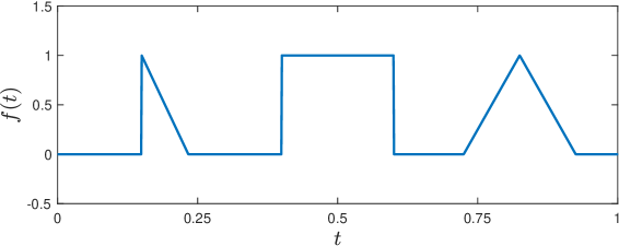
Figure 1: An example of a one-dimensional “image” $f(t)$. The vertical lines indicate jump discontinuities in $f$.

To blur this image, we will follow a simple idea:

replace the value $f(t)$ with a local average.

Since $f$ is a function of $t\in[0,1]$, its local average will be an integral over a small interval. Let us focus on some specific point $s\in[0,1]$, and suppose we want to blur $f(s)$ by averaging $f$ over the region $t\in[s-z,s+z]$ for some small value of $z>0$. Integrate $f$ over this interval, and divide by the width of the interval to get our first model for blurring a function:

$$b(s)=\frac{\mbox{area under $f(t)$ for $t\in[s-z,s+z]$}}{\mbox{width of interval $[s-z,s+z]$}}=\frac{1}{2z}\int_{s-z}^{s+z}f(t)\,{\rm d}t.$$ (1)

Think for a moment about the influence of the parameter $z$. How does $z$ affect the blurring? As $z$ increases, we average $f$ over a wider window; more distant points influence $b(s)$, resulting in a more severe blur. Figure 2 confirms this intuition, showing the affect of averaging the $f$ from Figure 1 over intervals of width $2z$ for $z=0.025$ and $z=0.05$.

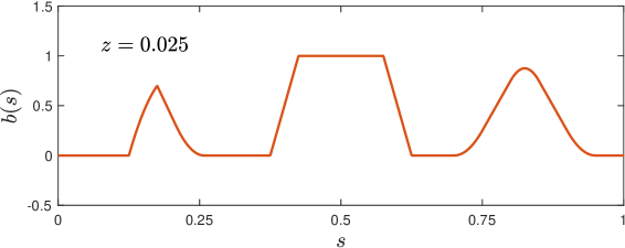
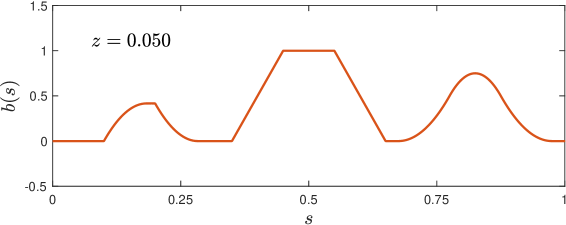
Figure 2: A blurred version of the image from Figure 1, using the simple blurring function (3) with parameter $z=0.025$ (top) and $z=0.05$ (bottom): the larger the value of $z$, the stronger the blurring effect.

We can use $z$ to adjust the severity of the blur, but still this model of blurring is quite crude. To facilitate more general models of blurring, realize that the integral in (1) can be written as

$$b(s)=\int_{0}^{1}h(s,t)\mkern 1.0muf(t)\,{\rm d}t,$$ (2)

where $h(s,t)$ is a function that controls how the blurring is computed. Such an $h(s,t)$ is called a kernel function. For the example in (1), we have the averaging kernel

$$\begin{array}[]{ll}\displaystyle{\kern-3.5pth(s,t)=\left\{\begin{array}[]{rl}\displaystyle{\frac{1}{2z},}&|t-s|\leq z;\\[9.0pt] 0,&|t-s|>z.\end{array}\right.}&\mbox{\begin{picture}(100.0,0.0)(0.0,5.0)\put(24.0,0.0){\includegraphics[width=72.26999pt]{IMAGES/cartoon_kernel_1}} \put(39.0,-4.5){\scriptsize{$s\kern-1.5pt-\kern-1.5ptz$}} \put(58.2,-4.5){\scriptsize{$s$}} \put(67.25,-4.5){\scriptsize{$s\kern-1.5pt+\kern-1.5ptz$}} \end{picture}}\end{array}$$ (3)

Consider how different choices of $h(s,t)$ can lead to different kinds of blurring. For example, in our initial model, $b(s)$ is influenced equally by $f(t)$ for all $t\in[s-z,s+z]$. Instead, we might expect $b(s)$ to be more heavily influenced by $f(t)$ for $t\approx s$, and less influenced by $f(t)$ when $t$ is far from $s$. We could accomplish this goal by using the hat-function kernel

$$\begin{array}[]{ll}\displaystyle{\kern 0.0pth(s,t)=\frac{1}{z}\max\Big{(}0,1-\frac{|t-s|}{z}\Big{)}}&\mbox{\begin{picture}(100.0,0.0)(0.0,14.0)\put(20.3,0.0){\includegraphics[width=72.26999pt]{IMAGES/cartoon_kernel_2}} \put(35.5,-4.5){\scriptsize{$s\kern-1.5pt-\kern-1.5ptz$}} \put(54.5,-4.5){\scriptsize{$s$}} \put(63.0,-4.5){\scriptsize{$s\kern-1.5pt+\kern-1.5ptz$}} \end{picture}}\end{array}$$ (4)

or the Gaussian kernel

$$\begin{array}[]{ll}\displaystyle{\kern-24.0pth(s,t)=\frac{1}{\sqrt{\pi}\mkern 1.0mu\mkern 1.0muz}{\rm e}^{-(t-s)^{2}/z^{2}}.}&\mbox{\begin{picture}(100.0,0.0)(0.0,7.0)\put(44.5,0.0){\includegraphics[width=72.26999pt]{IMAGES/cartoon_kernel_3}} \put(59.5,-4.5){\scriptsize{$s\kern-1.5pt-\kern-1.5ptz$}} \put(78.5,-4.5){\scriptsize{$s$}} \put(87.0,-4.5){\scriptsize{$s\kern-1.5pt+\kern-1.5ptz$}} \end{picture}}\end{array}$$ (5)

Figure 3 compares these three choices of $h(s,t)$ for $s=0.35$ with the two blurring parameters $z=0.05$ and $z=0.025$. (The larger $z$, the stronger the blur.) In a real experiment, we could potentially determine the best choice of kernel $h(s,t)$ and blurring factor $z$ by doing experiments with our camera, taking pictures of test patterns and measuring the resulting blur.

As the kernel $h(s,t)$ gets more sophisticated, so too does the calculus required to convert a signal $f(t)$ into its blurred version. Even more difficult is the task of taking a blurry image $b(s)$ and inverting the integration process to determine the unblurred image $f(t)$. To make such tasks computationally tractable, we will approximate the calculus problem with a simpler problem involving linear algebra.

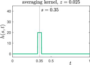
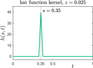
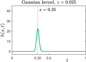
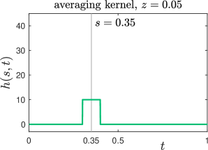
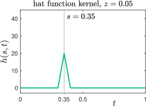
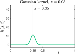
Figure 3: Three choices of the kernel function $h(s,t)$, centered at $s=0.35$. The top plots use the blurring parameter $z=0.025$; the bottom plots use $z=0.05$. As $z$ gets increases, the kernel spreads more around the point $s$, resulting in more blurring.

Questions for Reflection

• Can you think of any other good shapes for a blurring function?

• All the blurring functions described here are symmetric about the point $s$, which means that $h(s,s-\tau)=h(s,s+\tau)$ for all $\tau>0$. Can you design a blurring function $h(s,t)$ so that $b(s)$ in (1) only depends on values of $f(t)$ for $t\leq s$?

2. Turning calculus into linear algebra

The trick for turning calculus into linear algebra is a technique called discretization. (This practical approximation aligns very nicely with applications: typically we only know our “image” $f$ at discrete pixel locations, not as a continuous function $f(t)$ for all values of $t\in[0,1]$.) We shall convert the continuous real intervals $s\in[0,1]$ and $t\in[0,1]$ into sets of $n$ discrete points:

$$s_{j}=\frac{j-1/2}{n},\qquad t_{k}=\frac{k-1/2}{n},\hbox to0.0pt{\qquad$j,k=1,\ldots,n$.\hss}$$

Here $n>1$ is a positive integer describing how many discretization points we will use. For example, when $n=5$ we would have the points

$$s_{1}=0.10,\quad s_{2}=0.30,\quad s_{3}=0.50,\quad s_{4}=0.70,\quad s_{5}=0.90.$$

We will only compute the blurred values $b(s)$ of $f(t)$ at the grid points $s_{j}$, so equation (2) becomes

$$\kern-29.0ptb(s_{j})=\int_{0}^{1}h(s_{j},t)\mkern 1.0muf(t)\,{\rm d}t,\hbox to0.0pt{\kern 48.7pt$j=1,\ldots,n$.\hss}$$ (6)

We want to approximate $b(s_{j})$ by only accessing the original function $f(t)$ at the grid points $t_{k}$. You likely encountered this idea when you first learned about integration: you can approximate the area under the curve by the sum of the areas of some rectangles that touch the curve at a point. This construction is known as Riemann sum. As the rectangles get narrower, the mismatch in area decreases. We will use rectangles of width $1/n$, and center them at the values of $t_{k}$, a process known as the midpoint rule. Figure 4 shows a sketch of the process. (We could use a fancier method to approximate the integral, like the trapezoid rule or Simpson’s rule [10, chap. 7], but that would be tangential to our purpose here.)

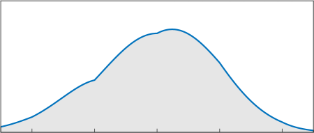
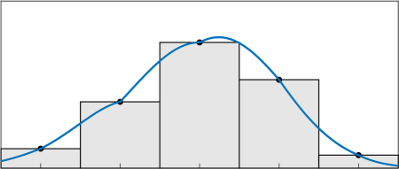
Figure 4: The integral (6) is the area under the blue curve $h(s_{j},t)f(t)$ in the left plot. Approximate this quantity with the area of the rectangles of width $1/n$ that touch $h(s_{j},t)f(t)$ at $t=t_{1},\ldots t_{n}$, as shown on the left and described in equation (7). This move allows us to replace a calculus problem with a linear algebra problem.

Applying the midpoint rule to (6) gives

$$b(s_{j})\approx\sum_{k=1}^{n}\frac{1}{n}\big{(}h(s_{j},t_{k})f_{k}\big{)}=:b_{j},\hbox to0.0pt{\qquad$j=1,\ldots,n$,\hss}$$ (7)

where $f_{k}=f(t_{k})$. Notice that we have introduced the notation $b_{j}$ to refer to the approximation to $b(s_{j})$ obtained by the midpoint rule.

Given this notation, you can regard $f_{k}$ as the intensity of the $k$th pixel in our “image;” similarly, $b_{j}$ represents the blurred value of the $j$th pixel. Our next challenge is to understand how the various $\{f_{k}\}$ values relate to the $\{b_{j}\}$ values.

Taking $j=1,\ldots,n$ gives us a set of $n$ equations that has a very regular structure:

$${1\over n}\big{(}h(s_{1},t_{1})f_{1}+h(s_{1},t_{2})f_{2}+\cdots+h(s_{1},t_{n})f_{n}\big{)} \;=\; b_{1}$$

$${1\over n}\big{(}h(s_{2},t_{1})f_{1}+h(s_{2},t_{2})f_{2}+\cdots+h(s_{2},t_{n})f_{n}\big{)} = b_{2}$$

$$\vdots$$

$${1\over n}\big{(}h(s_{n},t_{1})f_{1}+h(s_{n},t_{2})f_{2}+\cdots+h(s_{n},t_{n})f_{n}\big{)} = b_{n}.$$

We envision $n$ being a large number (we will use $n=500$ later), and so keeping track of these $n$ equations would be quite tedious. Thankfully the equations are all linear in the values $f_{1},\ldots,f_{n}$, and so we can collect these equations in a matrix-vector form:

$$\underbrace{{1\over n}\left[\begin{array}[]{cccc}h(s_{1},t_{1})&h(s_{1},t_{2})&\cdots&h(s_{1},t_{n})\\[2.5pt] h(s_{2},t_{1})&h(s_{2},t_{2})&\cdots&h(s_{2},t_{n})\\[2.5pt] \vdots&\vdots&\ddots&\vdots\\[2.5pt] h(s_{n},t_{1})&h(s_{n},t_{2})&\cdots&h(s_{n},t_{n})\end{array}\right]}_{\mbox{${\bf A}$}}\underbrace{\left[\begin{array}[]{c}f_{1}\\[2.5pt] f_{2}\\[2.5pt] \vdots\\[2.5pt] f_{n}\end{array}\right]}_{\mbox{${\bf f}$}}=\underbrace{\left[\begin{array}[]{c}b_{1}\\[2.5pt] b_{2}\\[2.5pt] \vdots\\[2.5pt] b_{n}\end{array}\right]}_{\mbox{${\bf b}$}}.$$ (8)

Thus, the $n$ equations in (7) can be expressed as the matrix-vector product ${\bf A}{\bf f}={\bf b}$. (Take note of the $1/n$ factor on the far left of (8): be sure to include it in the matrix ${\bf A}$, so that the $(j,k)$ entry is $a_{j,k}=h(s_{j},t_{k})/n$.)

The code in Figure 5 shows how to construct the matrix ${\bf A}$ in Python. Note that the function build_blur_A builds the matrix one row at a time, using only a single for loop. (This routine uses Gaussian blurring, but any other kernel could readily be swapped in.)

⬇

import numpy as np

def h_average(s,t,z=.025): # averaging kernel

return np.double(np.abs(s-t)<=z)/(2*z)

def h_hat(s,t,z=.025): # hat-function kernel

return np.maximum(0,1-np.abs(s-t)/z)/z

def h_gaussian(s,t,z=.025): # Gaussian kernel

c = 1/(np.sqrt(np.pi)*z)

return c*np.exp(-np.power(s-t,2)/(z**2))

def build_blur_A(n=100,z=.025):

A = np.zeros((n,n)); # n-by-n matrix of zeros

s = np.array([(j+.5)/n for j in range(n)]) # s_j points

t = np.array([(k+.5)/n for k in range(n)]) # t_k points

for j in range(0,n):

A[j,:] = h_gaussian(s[j],t,z)/n # A(j,k) = h(s_j,t_k)/n

return A

Figure 5: Python code to construct the three blurring functions (3), (4), and (5), and to build the matrix ${\bf A}$ defined in (8).

The matrix-vector form (8) has many advantages: for one thing, it provides a tidy way to organize the $n$ equations in $n$ unknown variables. The structure ${\bf A}{\bf f}={\bf b}$ encourages us think about the equation at a higher level of abstraction, enabling us to apply tools – both theoretical ideas and mathematical software – developed for general problems that share this same structure.

We can formulate a basic algorithm for approximating the blurring operation:

1. Select a grid size, $n$.

2. Construct the grid points, $t_{1},\ldots,t_{n}$.

3. Build the $n\times n$ matrix ${\bf A}$ from the blurring kernel $h(s,t)$.

4. Sample the function $f(t)$ at the grid points $t_{k}$, $k=1,\ldots,n$.
   Collect the results in the vector ${\bf f}\in\mathCR{R}^{n}$.

5. Compute the matrix-vector product ${\bf A}{\bf f}={\bf b}$ to find the blurred vector, ${\bf b}$.

Figure 6 shows how this blurring operation works for the hat-function kernel with $z=0.025$ and $n=100$. To the eye, the approximate blurring operation computed as ${\bf b}={\bf A}{\bf f}$ looks quite accurate. (Compare the bottom plot in Figure 6 to the top plot in Figure 2.)

We have seen how the calculus operation of blurring can be approximated by a basic linear algebra problem: blurring a signal reduces to simple matrix-vector multiplication. You can imagine applications where you would like to apply such blurring, e.g., obscuring the face of a bystander in a photograph of a crime scene. However, in many more situations we actually want to do the opposite of blurring: We acquire a blurry signal (from a camera, or a telescope) and we want to sharpen it up. We want to deblur. Linear algebra immediately suggests a way to do this: invert the blurring matrix. We will explore this possibility in the next section.

Questions for Reflection

• The most aggressive blurring you could imagine would simply take $h(s,t)=1$ for all $s,t\in[0,1]$. Describe the matrix ${\bf A}$ for this choice of blurring function. What would ${\bf b}={\bf A}{\bf f}$ look like? If you are given ${\bf f}$, could you solve for the unknown ${\bf b}$?

• The matrix ${\bf A}$ is said to be banded when $a_{j,k}=0$ provided $|j-k|$ is sufficiently large. Which of the three kernels studied in this section lead to a banded blurring matrix? How does the “width” of the band (the number of nonzeros per row) depend on $z$?

Now would be a good time to explore Exercises E2.1–E2.2 starting on page E2.1.

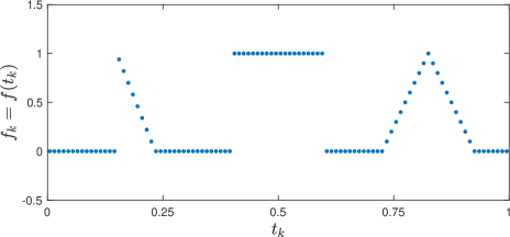
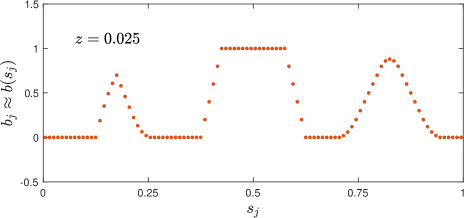
Figure 6: The original signal $f(t)$, sampled at $t=t_{k}$ for $k=1,\ldots,100=n$ (top), and the blurred values from ${\bf b}={\bf A}{\bf f}$, using the simple blurring kernel (3) with $z=0.025$. Compare these discretized versions to the continuous (exact) versions in Figure 1 and the top of Figure 2.

3. The inverse problem: deblurring

In the last section we saw the blurring operation described by ${\bf A}{\bf f}={\bf b}$, and we used knowledge of the blurring operation ${\bf A}$ and the original signal ${\bf f}$ to compute the blurry ${\bf b}$. This set-up is called the forward problem.

But now let us turn the tables. Suppose we acquire (that is, we measure) some blurry signal ${\bf b}$, and want to recover the unknown sharp signal, ${\bf f}$. We want to deblur ${\bf b}$. Linear algebra gives an immediate way to accomplish this goal: If ${\bf A}{\bf f}={\bf b}$, then we should have

$${\bf f}={\bf A}{\kern-1.0pt}^{-1}{\bf b},$$ (9)

provided ${\bf A}\in\mathCR{R}^{n\times n}$ is an invertible matrix. Since (9) involves the inverse of the blurring operation ${\bf A}$, we call this deblurring process an inverse problem. What could go wrong with the clean formula (9)?

We must first acknowledge that the ${\bf A}{\bf f}={\bf b}$ model is only a rough description of the true process of blurring. Here are a few ways the model falls short.

• The integral model in (2) is an imperfect description of the blurring process.

• The kernel $h(s,t)$ and the blurring parameter $z$ are only estimates of the properties of the instrument (camera, environmental conditions, etc.).

• The discretization process that turned (2) into the linear algebra problem (8) introduced an additional approximation.

• Measurements of the vector ${\bf b}$ (e.g., with a camera, telescope, or microscope) will inevitably be imperfect, adding a layer of (hopefully random) errors that we will call “noise.”

Humbled by this list of shortcomings, we might wonder if our model is any good at all! Indeed, simple computational experiments do little to build our confidence. Let us focus on the last flaw on our list, measurement errors in ${\bf b}$. Return to the example shown in Figure 6, but suppose that instead of exactly measuring ${\bf b}$, we acquire some noisy version, ${\bf b}_{\rm noise}$. Let the $j$th entry of this vector be

$$({\bf b}_{\rm noise})_{j}=b_{j}+e_{j},$$

where $b_{j}$ is the $j$th entry of ${\bf b}$ and $e_{j}$ is a normal random variable of mean zero and standard deviation $\varepsilon\|{\bf b}\|$, for some small value of $\varepsilon$. We are using the Euclidean vector norm defined by

$$\|{\bf b}\|=\sqrt{{\bf b}^{T}{\bf b}}=\Big{(}\sum_{j=1}^{n}b_{j}^{2}\Big{)}^{1/2},$$

so that the magnitude of the noise that pollutes ${\bf b}_{\rm noise}$ is calibrated to match the magnitude of ${\bf b}$.

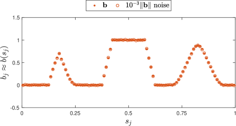
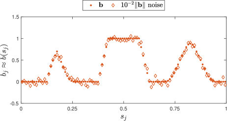
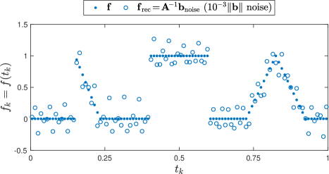
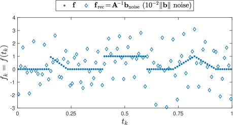
Figure 7: An attempt to recover ${\bf f}$ from noisy measurements ($n=100$, averaging kernel (3) with $z=0.025$). The true ${\bf b}={\bf A}{\bf f}$ is polluted with some random noise (normally distributed, mean zero, standard deviation $10^{-3}\|{\bf b}\|$ (left) or $10^{-2}\|{\bf b}\|$ (right)), giving ${\bf b}_{\rm noise}$. As seen in the top figures, ${\bf b}_{\rm noise}$ differs very little from ${\bf b}$ for both noise levels. We then recover the unblurred signal by computing ${\bf f}_{\rm rec}={\bf A}{\kern-1.0pt}^{-1}{\bf b}_{\rm noise}$. As seen in the bottom figures, a whiff of noise in ${\bf b}$ causes a large change to the recovered ${\bf f}$. The values in ${\bf f}_{\rm rec}$ ($\circ$ and $\diamond$) should fall on top of the true values in ${\bf f}$ ($\bullet$), but most are far from correct.

We might instinctively expect that an error of relative size $\varepsilon$ in ${\bf b}_{\rm noise}$ will cause an error of similar error in ${\bf f}_{\rm rec}={\bf A}{\kern-1.0pt}^{-1}{\bf b}_{\rm noise}$. Figure 7 shows that this is far from the case! Errors with $\varepsilon=10^{-3}$ and $\varepsilon=10^{-2}$ in ${\bf b}_{\rm noise}$ (just $0.1\%$ and $1.0\%$ relative noise level) cause much larger errors in ${\bf f}_{\rm rec}$. The crisp image ${\bf f}$ is not recovered at all; the recovered values are bad for $\varepsilon=10^{-3}$ and entirely useless for $10^{-2}$. (Indeed, the blurry, noisy version ${\bf b}_{\rm noise}$ gives us a better impression of the true ${\bf f}$ than the supposedly “deblurred” vector ${\bf f}_{\rm rec}$ does!) Lest one think there is something special about this particular example, in Figure 8 we repeat the experiment on a larger problem $(n=500)$ with the hat-function kernel (4) with $z=0.05$. Even the noise level $10^{-5}\|{\bf b}\|$ causes catastrophic errors in ${\bf f}_{\rm rec}={\bf A}{\kern-1.0pt}^{-1}{\bf b}_{\rm noise}$.

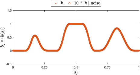
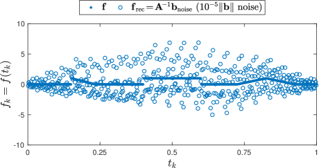
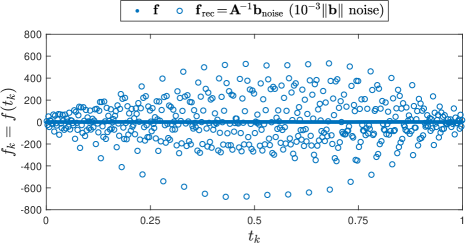
Figure 8: Repetition of Figure 7, but now using $n=500$ with the hat-function kernel (4) with $z=0.05$ and noise levels $10^{-5}\|{\bf b}\|$ (left) and $10^{-3}\|{\bf b}\|$ (right). The very subtle level of noise in ${\bf b}_{\rm noise}$ on the top-left is essentially unnoticeable to the eye, yet it causes profound errors in ${\bf f}_{\rm rec}$ in the bottom-left plot. When the noise increases by two orders of magnitude (top-right), so too do the errors in ${\bf f}_{\rm rec}$.

It is tempting to conclude that we need better measurements, that the problem can be overcome if we can only obtain greater precision. However, the quest for more precision is a fool’s errand. The difficulty exposed by this simple example is chronic, becoming increasingly problematic for more realistic signals and blurring kernels. Figure 9 shows such an example, reflecting the kinds of barcodes that we will focus upon later in this manuscript. In this case we start with a vector ${\bf f}\in\mathCR{R}^{570}$ containing only the values zero and one. Using the Gaussian kernel (5) with $z=0.01$, we blur this function to obtain ${\bf b}={\bf A}{\bf f}$. Now without injecting any intentional noise, we simply try to undo this matrix vector product: ${\bf f}_{\rm rec}={\bf A}{\kern-1.0pt}^{-1}{\bf b}$. The small numerical rounding errors that occur when we compute with double-precision floating point arithmetic are sufficient to make the inversion process go haywire: while we hope for ${\bf f}_{\rm rec}$ to be a vector containing only zeros and ones, ${\bf f}_{\rm rec}$ contains much larger values – indeed, values over 100 times too large.

In the face of such failure we might be tempted to give up (or look for a bug in our code). Instead, we will use this as an opportunity to gain insight into the subtlety of matrix inversion, and to find a more robust approach to solving this kind of fragile inverse problem.

the barcode
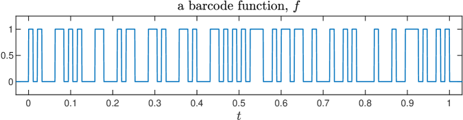
  the original function
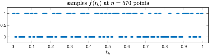
  sample $f$ at $t_{k}$ to get ${\bf f}$
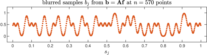
  blur ${\bf f}$ to get ${\bf b}={\bf A}{\bf f}$ Gaussian blur (5) with $z=0.01$
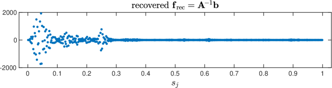
  undo the blur ${\bf f}_{\rm rec}={\bf A}{\kern-1.0pt}^{-1}{\bf b}$ (We should get ${\bf f}_{\rm rec}={\bf f}$.)

Figure 9: Deblurring our first barcode. A Universal Product Code (UPC) is shown at the top. We translate this barcode into a function $f$ that takes values 0 (white bar) and 1 (black bar). When sampled on a grid of $n=570$ points, the vector ${\bf f}\in\mathCR{R}^{570}$ only contains the values zero and one. Blur this vector using the Gaussian kernel (5) with $z=0.01$ to get ${\bf b}={\bf A}{\bf f}$, shown in red. Attempt to undo the blur by computing ${\bf f}_{\rm rec}={\bf A}{\kern-1.0pt}^{-1}{\bf b}$. Instead of recovering the true ${\bf f}$ (zeros and ones), we get much larger values! Though we have not injected any extra noise, the inversion process is sufficiently sensitive to small numerical errors to make the result useless.

Questions for Reflection

• In this section we suggest four potential sources of error in the modeling process. Which of these do you think is most significant, and which least significant? Can you think of any other sources of error that we have not mentioned?

• Can you imagine two vectors ${\bf f}_{1}\not\approx{\bf f}_{2}$ that would be very similar when blurred? That is, ${\bf A}{\bf f}_{1}\approx{\bf A}{\bf f}_{2}$? (Another way of thinking about this question: Is there a vector ${\bf z}$ that gets blurred to almost nothing: ${\bf A}{\bf z}\approx{\bf 0}$? In that case, set ${\bf f}_{2}={\bf f}_{1}+{\bf z}$.)

Now would be a good time to explore Exercises E3.1–E3.3 starting on page E3.1.

4. What is wrong with ${\bf A}{\kern-1.0pt}^{-1}$?

The image deblurring failure has an intuitive explanation. Think about blurring a photograph. Sharp lines are smoothed; fine distinguishing features often wash out. Two similar images that have distinct details could look nearly identical once they are blurred. We are asking the inversion process to recover those fine details that are obscured by the blurring, a challenging task.

While this explanation might make intuitive sense, we can better understand the issue through the language of linear algebra, and we do not need anything as complicated as a blurring matrix to see what is going on. Instead, consider the simple $2\times 2$ matrix

$${\bf A}=\left[\begin{array}[]{cc}1&-0.05\\ 1&\phantom{-}0.05\end{array}\right].$$

This matrix has two linearly independent columns and two linearly independent rows; the rank of the matrix is two, and it is invertible: $\det({\bf A})=0.10\neq 0$. Indeed, you can compute

$${\bf A}{\kern-1.0pt}^{-1}=\left[\begin{array}[]{rr}0.5&0.5\\ -10&\phantom{-}10\end{array}\right].$$

Notice that ${\bf A}$ is an invertible matrix, but the rows of ${\bf A}$ are nearly linearly dependent. (Think about plotting those two vectors – they point in nearly the same direction.) Even though the largest entry in ${\bf A}$ is 1, ${\bf A}{\kern-1.0pt}^{-1}$ has entries that are 10 times as large. Figure 10 illustrates the implications. Consider the blue patch on the left, which contains all vectors of the form

$${\bf f}=\left[\begin{array}[]{c}\alpha\\ \beta\end{array}\right]$$

that fall within a disk of radius 0.25 centered at $[1,1]^{T}$; i.e.,

$$|\alpha-1|^{2}+|\beta-1|^{2}\leq 0.25.$$

The matrix ${\bf A}$ maps these vectors to the red patch on the right, a narrow ellipse. Two representative vectors ${\bf f}_{1}$ and ${\bf f}_{2}$ are far apart (in the plot on the left), but they are mapped quite close together by ${\bf A}$, so that ${\bf b}_{1}={\bf A}{\bf f}_{1}$ and ${\bf b}_{2}={\bf A}{\bf f}_{2}$ appear nearby (in the plot on the right).

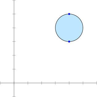
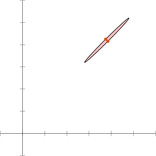
Figure 10: On the left, the domain ${\bf f}\in\mathCR{R}^{2}$, with a ball of ${\bf f}$ vectors highlighted in blue. On the right, the image ${\bf A}{\bf f}\in\mathCR{R}^{2}$, with the red ellipse showing the image of the blue disk on the left. Note that the two vectors ${\bf f}_{1}$ and ${\bf f}_{2}$ are distant, but their images ${\bf A}{\bf f}_{1}$ and ${\bf A}{\bf f}_{2}$ are quite close.

Now imagine we make a small change to

$${\bf b}_{1}={\bf A}{\bf f}_{1}=\left[\begin{array}[]{cc}1&-0.05\\ 1&\phantom{-}0.05\end{array}\right]\left[\begin{array}[]{c}1\\ 1.25\end{array}\right]=\left[\begin{array}[]{c}0.9375\\ 1.0625\end{array}\right]$$

to obtain

$${\bf b}_{\rm noise}={\bf b}_{1}+{\bf e}=\left[\begin{array}[]{c}0.9375\\ 1.0625\end{array}\right]+\left[\begin{array}[]{r}0.0125\\ -0.0125\end{array}\right]=\left[\begin{array}[]{c}0.95\\ 1.05\end{array}\right].$$

Then when we “recover” ${\bf f}_{1}$ from ${\bf b}_{\rm noise}$, we obtain

$${\bf f}_{\rm rec}={\bf A}{\kern-1.0pt}^{-1}{\bf b}_{\rm noise}=\left[\begin{array}[]{rr}0.5&0.5\\ -10&\phantom{-}10\end{array}\right]\left[\begin{array}[]{c}0.95\\ 1.05\end{array}\right]=\left[\begin{array}[]{c}1.00\\ 1.00\end{array}\right]\neq\left[\begin{array}[]{c}1\\ 1.25\end{array}\right]={\bf f}_{1}.$$

Changing the entries of ${\bf b}_{1}$ by just $\pm 0.0125$ changed the recovered signal ${\bf f}_{\rm rec}$ by $0.25$ in the second entry. As the next exercise shows, even in this simple $2\times 2$ matrix example, we can adjust the entries of ${\bf A}$ to make the discrepancy between ${\bf f}_{\rm rec}$ and ${\bf f}_{1}$ arbitrarily large.

Question for Reflection

• The theme of this section is that multiplication by ${\bf A}^{-1}$ can map close-together vectors ${\bf b}_{1}$ and ${\bf b}_{2}$ to far-away vectors ${\bf f}_{1}={\bf A}^{-1}{\bf b}_{1}$ and ${\bf f}_{2}={\bf A}^{-1}{\bf b}_{2}$.

  Can you apply this same concept to functions of a single real variable, $g(x):\mathCR{R}\to\mathCR{R}$? That is, can you find a function $g$ such that $g(x+h)$ is very different from $g(x)$ for small values of $|h|>0$? How does this relate to the derivative $g^{\prime}(x)$?

Now would be a good time to explore Exercise E4.1 on page E4.1.

5. A Remedy from Regularization

We have sought to compute ${\bf f}$ as the unique solution to the linear system

$${\bf A}{\bf f}={\bf b},$$

which we simply write as

$${\bf f}={\bf A}{\kern-1.0pt}^{-1}{\bf b}.$$

When we try to compute the “exact solution” ${\bf f}$ and get some nonsensical values (like we saw in Figure 9), we realize that satisfying the linear system ${\bf A}{\bf f}={\bf b}$ is only one of our objectives. We also want ${\bf f}$ to have realistic, meaningful entries. For example, when solving the barcode problem, we might ask for every entry of ${\bf f}$ to be either zero or one. (For reasons not immediately obvious, this turns out to be quite a difficult condition to impose, computationally.) A simpler requirement is to simply ask that $\|{\bf f}\|$ not be too large.

So, we want ${\bf A}{\bf f}\approx{\bf b}$ while keeping $\|{\bf f}\|$ as small as possible. Let us introduce a parameter $\lambda>0$, and define an objective function that balances these two requirements:

$$\phi({\bf f})=\|{\bf b}-{\bf A}{\bf f}\|^{2}+\lambda^{2}\|{\bf f}\|^{2}.$$ (10)

Our goal is to find the ${\bf f}\in\mathCR{R}^{n}$ that minimizes $\phi({\bf f})$.

The act of penalizing the misfit $\|{\bf b}-{\bf A}{\bf f}\|$ with some term that controls the size of the solution (such as $\|{\bf f}\|$) is known as regularization. More specifically, mathematicians see the optimization of the objective function (10) as an example of Tikhonov regularization, while statisticians call this approach ridge regression.

What role does the parameter $\lambda$ play? Consider the extreme choices.

• By setting $\lambda=0$, we entirely neglect $\|{\bf f}\|$, placing all our emphasis on making ${\bf A}{\bf f}={\bf b}$. (Indeed, this was our initial strategy, above: take ${\bf f}={\bf A}{\kern-1.0pt}^{-1}{\bf b}$.)

• By taking $\lambda\to\infty$, we place increasing importance on controlling $\|{\bf f}\|$, while neglecting ${\bf A}{\bf f}={\bf b}$. In the limit $\lambda\to\infty$, we would simply obtain ${\bf f}={\bf 0}$: a solution that indeed makes $\|{\bf f}\|$ small, but is not interesting as a solution to ${\bf A}{\bf f}\approx{\bf b}$.

How can we minimize $\phi({\bf f})$? We will approach the question from the perspective of multivariable calculus. (One can derive the same solution using only properties of linear algebra; see, e.g., [1, chap. 7].) To minimize a smooth function $\phi({\bf f})$, we should take the gradient (with respect to ${\bf f}$), set this gradient equal to zero, and solve for ${\bf f}$. Recalling that we can expand norms using inner products (e.g., $\|{\bf y}\|^{2}={\bf y}^{T}{\bf y}$) and distribute inner products (e.g., $({\bf x}+{\bf y})^{T}{\bf z}={\bf x}^{T}{\bf z}+{\bf y}^{T}{\bf z}$), we can write:

$$\phi({\bf f}) = \|{\bf b}-{\bf A}{\bf f}\|^{2}+\lambda^{2}\mkern 1.0mu\|{\bf f}\|^{2}$$ (11)

$$= ({\bf b}-{\bf A}{\bf f})^{T}({\bf b}-{\bf A}{\bf f})+\lambda^{2}\mkern 1.0mu\mkern 1.0mu{\bf f}^{T}{\bf f}$$

$$= {\bf b}^{T}{\bf b}-2\mkern 1.0mu\mkern 1.0mu{\bf f}^{T}{\bf A}{\kern-1.0pt}^{T}{\bf b}+{\bf f}^{T}{\bf A}{\kern-1.0pt}^{T}\!{\bf A}{\bf f}+\lambda^{2}\mkern 1.0mu\mkern 1.0mu{\bf f}^{T}{\bf f}.$$ (12)

Compute the gradient of $\phi$ with respect to the variable ${\bf f}$, recalling that $\lambda$ is a constant:

$$\nabla\phi({\bf f}) = {\bf 0}-2{\bf A}{\kern-1.0pt}^{T}{\bf b}+2\mkern 1.0mu{\bf A}{\kern-1.0pt}^{T}\!{\bf A}{\bf f}+2\lambda^{2}\mkern 1.0mu\mkern 1.0mu{\bf f}$$ (13)

$$= 2({\bf A}{\kern-1.0pt}^{T}{\bf A}{\bf f}+\lambda^{2}\mkern 1.0mu\mkern 1.0mu{\bf f}-{\bf A}{\kern-1.0pt}^{T}{\bf b}).$$

To find critical points of $\phi$, set $\nabla\phi({\bf f})={\bf 0}$ and solve for ${\bf f}$. Thus we find that ${\bf A}{\kern-1.0pt}^{T}{\bf A}{\bf f}+\lambda^{2}\mkern 1.0mu\mkern 1.0mu{\bf f}={\bf A}{\kern-1.0pt}^{T}{\bf b}$, i.e.,

$$\big{(}{\bf A}{\kern-1.0pt}^{T}\!{\bf A}+\lambda^{2}{\bf I}){\bf f}={\bf A}{\kern-1.0pt}^{T}{\bf b}.$$ (14)

We denote the solution for this fixed value of $\lambda$ as

$${\bf f}_{\lambda}:=({\bf A}{\kern-1.0pt}^{T}\!{\bf A}+\lambda^{2}{\bf I})^{-1}{\bf A}{\kern-1.0pt}^{T}{\bf b}.$$ (15)

Notice that if ${\bf A}$ is invertible and we take $\lambda=0$, we get

$${\bf f}_{\mkern 1.0mu0}\ =\ ({\bf A}{\kern-1.0pt}^{T}\!{\bf A})^{-1}{\bf A}{\kern-1.0pt}^{T}{\bf b}\ =\ {\bf A}{\kern-1.0pt}^{-1}{\bf A}{\kern-1.0pt}^{-T}{\bf A}{\kern-1.0pt}^{T}{\bf b}\ =\ {\bf A}{\kern-1.0pt}^{-1}{\bf b},$$

and so this approach recovers the original solution (9). When $\lambda>0$, the $\lambda^{2}{\bf I}$ term in (15) increases all the diagonal entries of ${\bf A}{\kern-1.0pt}^{T}\!{\bf A}+\lambda^{2}{\bf I}$, making the rows and columns increasingly distinct from one another. This enhancement adds robustness to the inversion process – although when $\lambda$ is too large the $\lambda^{2}\mkern 1.0mu{\bf I}$ term will dominate the ${\bf A}{\kern-1.0pt}^{T}{\bf A}$ term, resulting in an ${\bf f}$ that makes $\|{\bf b}-{\bf A}{\bf f}\|$ unacceptably large.

Perhaps it is tempting to implement the formula (15) by computing the inverse of the $n\times n$ matrix ${\bf A}{\kern-1.0pt}^{T}{\bf A}+\lambda^{2}\mkern 1.0mu{\bf I}$, and then multiplying the result against ${\bf b}$. Instead, it is again more efficient to solve a linear system of equations using Gaussian elimination.

⬇

lam = 1e-5; % regularization parameter

I = np.identity(n) % n-by-n identity matrix

flam = np.linalg.solve(A.T@A+(lam**2)*I,(A.T)@b) % solve linear system

For subtle numerical reasons, one actually prefers to set this problem up a little bit differently. As will be derived in an exercise at the end of this section, one can pose the objective function (10) as a standard linear least squares problem of the form

$$\min_{{\bf f}\in\mathCR{R}^{n}}\phi({\bf f})=\min_{{\bf f}\in\mathCR{R}^{n}}\left\|\left[\begin{array}[]{c}{\bf b}\\ {\bf 0}\end{array}\right]-\left[\begin{array}[]{c}{\bf A}\\ \lambda\mkern 1.0mu{\bf I}\end{array}\right]{\bf f}\;\right\|.$$ (16)

We will denote the augmented matrix and vector in this equation as

$${\bf A}_{\lambda}=\left[\begin{array}[]{c}{\bf A}\\ \lambda\mkern 1.0mu{\bf I}\end{array}\right]\in\mathCR{R}^{2n\times n},\qquad{\bf b}_{\lambda}=\left[\begin{array}[]{c}{\bf b}\\ {\bf 0}\end{array}\right]\in\mathCR{R}^{2n}.$$

In Python, one can solve the least squares problem (16) using the np.linalg.lstsq command. (Other languages provide similar functionality; e.g., in MATLAB, flam = Alam\blam.)

⬇

lam = 1e-5; % regularization parameter

I = np.identity(n) % n-by-n identity matrix

Alam = np.block([[A],[lam*I]])

blam = np.block([b,np.zeros(n)])

flam = np.linalg.lstsq(Alam,blam,rcond=None)[0] % solve least squares problem

Figure 11 revisits the example on the left side of Figure 8, where a whiff of noise (standard deviation $10^{-5}\|{\bf b}\|$) was enough to entirely break our initial recovery attempt, ${\bf f}_{\rm rec}={\bf A}{\kern-1.0pt}^{-1}{\bf b}_{\rm noise}$. Now we attempt to recover the signal using regularization, ${\bf f}_{\lambda}=({\bf A}{\kern-1.0pt}^{T}{\bf A}+\lambda^{2}{\bf I})^{-1}{\bf b}_{\rm noise}$ for six different values of the regularization parameter $\lambda$. When $\lambda$ is too small, regularization has little effect on ${\bf f}_{\lambda}$; when $\lambda$ is too large, the solution is suppressed. Between these extremes the regularization gives an improved solution over the ${\bf f}={\bf A}{\kern-1.0pt}^{-1}{\bf b}$ solution we saw in Figure 8.

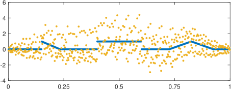
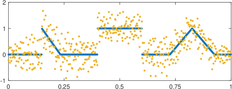
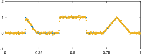
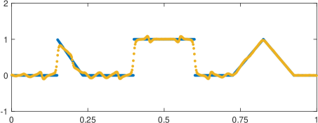
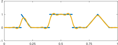
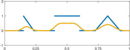
Figure 11: Six attempts to recover ${\bf f}$ from ${\bf b}_{\rm noise}$ polluted with random noise (normally distributed, mean zero, standard deviation $10^{-5}\|{\bf b}\|$), using grid of $n=500$ points with the hat-function blurring kernel (4) using $z=0.05$. The blue points show the true vector ${\bf f}$ that we are trying to recover; the yellow points show ${\bf f}_{\lambda}$ for the various $\lambda$ values. When $\lambda$ is too small (top left), the regularization term $\lambda^{2}\|{\bf f}\|^{2}$ has little effect, and the resulting ${\bf f}_{\lambda}$ is poor; when $\lambda$ is too large (bottom right), ${\bf f}_{\lambda}$ is excessively suppressed. The intermediate values $\lambda=10^{-2}$ and $\lambda=10^{-1}$ do a better (but not perfect) job of recovering the true signal.

Figure 12 shows the regularized solutions for the barcode deblurring problem introduced in Figure 9, but now using ${\bf b}_{\rm noise}$ with noise level $10^{-8}\|{\bf b}\|$. Recall that in this case the true solution ${\bf f}\in\mathCR{R}^{570}$ is a binary vector (all entries are either zero or one), and so it suffices to recover a solution ${\bf f}_{\lambda}$ for which we can decide if $f_{j}=0$ or $f_{j}=1$. For example, for each $\lambda$ we could set a threshold at the average of the extreme values computed in the vector ${\bf f}_{\lambda}$,

$$\tau_{\lambda}:=\frac{1}{2}\Big{(}{\displaystyle\min_{1\leq j\leq n}({\bf f}_{\lambda})_{j}\ +\ \max_{1\leq j\leq n}({\bf f}_{\lambda})_{j}}\Big{)},$$

and then draw a vertical black bar at $t_{j}\in[0,1]$ if $({\bf f}_{\lambda})_{j}\geq\tau_{\lambda}$ for $j=1,\ldots,n$. The barcodes on the right of Figure 12 are the result. Again we see that taking $\lambda$ too small does not sufficiently regularize the solution, and the resulting barcode is nonsense. Taking $\lambda$ too large pushes the values in ${\bf f}_{\lambda}$ too close to zero, also giving a ridiculous solution. The best choices for $\lambda$ lie in between these extremes. While none of three values $\lambda=10^{-7}$, $10^{-5}$, and $10^{-3}$ recover the function $f$ perfectly, using the $\tau_{\lambda}$ threshold allows us to recover the bar code quite reliably in all three cases. (The $10^{-7}$ result is off in just three of the $n=570$ positions; the $10^{-5}$ and $10^{-3}$ results match perfectly.)

When we compare the two deblurring examples shown in Figures 11 and 12, we notice that several of the “good” values of $\lambda$ for the barcode example (Figure 12) would would have been much too small for the problem shown in Figure 11. Clearly there is some nuance to the choice of $\lambda$, and we should not expect one magical value of $\lambda$ to work for all problems we encounter. What guidance can we find for selecting this crucial parameter? We will explore this question in the next section.

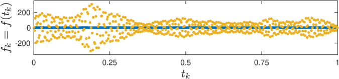
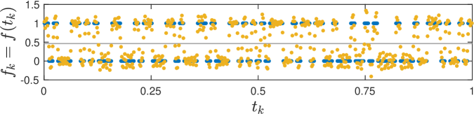
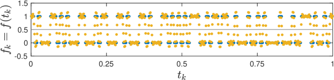
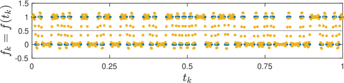
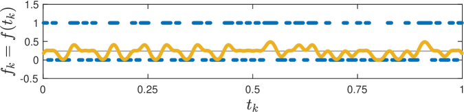
Figure 12: Barcode deblurring with the help of regularization, again with $n=570$ and the Gaussian kernel (5) with $z=0.01$. We inject some random noise (size $10^{-8}\|{\bf b}\|$) to get ${\bf b}_{\rm noise}$, and use regularization to recover ${\bf f}_{\lambda}$ for five values of $\lambda$. The yellow points show ${\bf f}_{\lambda}$; the blue points show the true values of ${\bf f}$. In each case, we translate ${\bf f}_{\lambda}$ into a barcode by letting each entry above the midpoint of the extreme values of ${\bf f}_{\lambda}$ correspond to a black bar. (This threshold is shown as the gray horizontal line visible on the bottom four plots.) The value $\lambda=10^{-10}$ is too small to tame the unruly solution, and the barcode looks nothing like the correct version seen atop Figure 9. The intermediate values $\lambda=10^{-7}$, $\lambda=10^{-5}$, and $\lambda=10^{-3}$ all do a reasonable job of recovering the desired barcode. The large value $\lambda=10^{0}$ puts too much emphasis on minimizing $\|{\bf f}\|$ and not enough on making ${\bf A}{\bf f}\approx{\bf b}$, resulting in a poor solution.

Questions for Reflection

• Explain, in careful detail, how to move from (11) to (12) in the derivation of the formula for $\phi({\bf f})$.

• When solving a modeling problem, it is often easy to fixate on minimizing an objective function, like $\|{\bf b}-{\bf A}{\bf f}\|$, without thinking about what that means for the motivating application. For the barcode problem, which goal is more important: getting an exact solution ${\bf f}$ to ${\bf A}{\bf f}={\bf b}$, or getting an approximate solution ${\bf f}$ that is good enough for you to recover the barcode exactly?

Now would be a good time to explore Exercises E5.1–E5.2 starting on page E5.1.

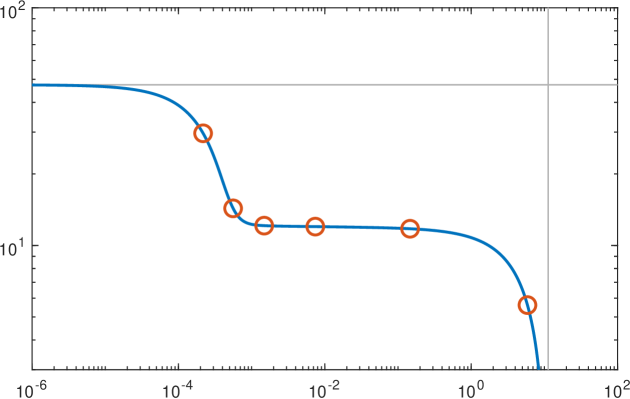
Figure 13: An “L curve” corresponding to the example in Figure 11. The goal of regularization is to choose a value of $\lambda$ that balances the goals of minimizing $\|{\bf b}_{\rm noise}-{\bf A}{\bf f}_{\lambda}\|$ while controlling $\|{\bf f}_{\lambda}\|$. Appealing values of $\lambda$ typically fall near the central bend in this curve (near $\lambda=10^{-3}$ on this plot).

6. Choosing the regularization parameter

As suggested by Figures 11 and 12, selection of the regularization parameter can be somewhat subtle. The optimal choice will depend on the application and the data. Are you willing to accept a solution that exhibits a bit of chatter, but captures edges well (as for $\lambda=10^{-3}$ in Figure 11), or do you want to suppress the noise at the cost of an overly smooth solution (as for $\lambda=10^{-2}$ or $\lambda=10^{-3}$ in Figure 11)? While various sophisticated approaches exist to guide the selection of $\lambda$ (see [2, sect. 6.4.1] and [5] for some details), in this manuscript we will only explore trial-and-error investigations.

How does the balance between $\|{\bf b}-{\bf A}{\bf f}_{\lambda}\|$ and $\|{\bf f}_{\lambda}\|$ tilt, as $\lambda$ increases from $\lambda=0$ to $\lambda\to\infty$? To see how this relationship evolves, you can solve the regularization problem for a wide range of $\lambda$ values, and then create a plot of the ordered pairs $(\|{\bf b}-{\bf A}{\bf f}_{\lambda}\|,\|{\bf f}_{\lambda}\|)$. Because these quantities can vary over several orders of magnitude, it is helpful to draw this as a log-log plot (i.e., plotting the pairs $(\log_{10}\|{\bf b}-{\bf A}{\bf f}_{\lambda}\|,\log_{10}\|{\bf f}_{\lambda}\|)$. Figure 13 shows a representative plot generated for the problem shown in Figure 11, while Figure 14 shows the analogous plot for the barcode regularization problem in Figure 12.

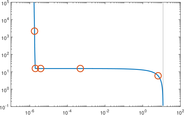
Figure 14: An “L curve” corresponding to the example in Figure 12. The three intermediate values of $\lambda$ that lead to a reasonable recovery of the barcode ($\lambda=10^{-7},10^{-5},10^{-3}$) all fall on the plateau of the L shape, with $10^{-7}$ very close to the corner. This plot makes clear that $\lambda=10^{-10}$ fails to control $\|{\bf f}_{\lambda}\|$, while $\lambda=10^{0}$ permits $\|{\bf b}_{\rm noise}-{\bf A}{\bf f}_{\lambda}\|$ to be too large.

Such plots are called “L curves,” named for the prominent central bend that these plots often (but not always) exhibit. As $\lambda$ increases from $0\to\infty$, the plot moves from the top-left to the bottom-right. The “L” shows the transition from a vertical drop (where small increases in $\lambda$ give big, desirable reductions in $\|{\bf f}_{\lambda}\|$ without much increase in the misfit $\|{\bf b}-{\bf A}{\bf f}_{\lambda}\|$) toward a horizontal plateau (where further increases in $\lambda$ give modest reductions in $\|{\bf f}_{\lambda}\|$ but undesirably large increases in $\|{\bf b}-{\bf A}{\bf f}_{\lambda}\|$).

When you first encounter an L curve, the plot can be a little tricky to understand. First off, appreciate that you cannot directly read off the values for $\lambda$ from the horizontal or vertical axes. You need to plot some test values of $(\|{\bf b}-{\bf A}{\bf f}_{\lambda}\|,\|{\bf f}_{\lambda}\|)$ to appreciate how $\lambda$ changes along the curve. (The red circles in Figures 13 and 14 show the points on the L curve corresponding to the $\lambda$ values used to compute the solutions shown in Figures 11 and 12.) Now look for several landmark features on the L curve.

• As $\lambda\to 0$, the optimization places diminishing emphasis on $\|{\bf f}_{\lambda}\|$; it primarily minimizes $\|{\bf b}-{\bf A}{\bf f}_{\lambda}\|$. For $\lambda=0$ the minimum is attained by ${\bf f}_{\rm rec}={\bf A}{\kern-1.0pt}^{-1}{\bf b}$, which gives ${\bf b}-{\bf A}{\bf f}_{\rm rec}={\bf 0}$. Look for the horizontal asymptote at the level $\|{\bf f}_{\rm rec}\|$ at the top-left of the L curve, visible in Figure 13.

• As $\lambda\to\infty$, the optimization completely focuses on minimizing $\|{\bf f}_{\lambda}\|$, and so ${\bf f}_{\lambda}\to{\bf 0}$ as $\lambda\to\infty$. Thus, as $\lambda$ gets large $\|{\bf b}-{\bf A}{\bf f}_{\lambda}\|\to\|{\bf b}\|$. This limit is seen on the bottom-right of Figures 13 and 14.

Sitting between these extremes, the corner of the L is a “sweet spot” where the goals of minimizing both $\|{\bf f}_{\lambda}\|$ and $\|{\bf b}-{\bf A}{\bf f}_{\lambda}\|$ are balanced. Due to the logarithmic nature of the axes, choosing $\lambda$ even a bit before the corner (i.e., too small) can yield a poor solution due to the large value of $\|{\bf f}_{\lambda}\|$, whereas choosing $\lambda$ a bit after the corner increases $\|{\bf b}-{\bf A}{\bf f}_{\lambda}\|$, but often not in a problematic way. Consider the barcode example from Figure 14, where we know the entries of the true solution ${\bf f}$ must be 0 or 1. In this case, a factor of 10 difference in $\|{\bf f}_{\lambda}\|$ (say, $10^{1}$ versus $10^{2}$) has a significant impact on the quality of the recovered solution; however, a factor of 10 difference in the small values of $\|{\bf b}-{\bf A}{\bf f}_{\lambda}\|$ (say, from $10^{-5}$ to $10^{-4}$) will hardly be noticeable in plots of the solution.

The following code will produce an L curve like the one shown in Figure 13 (presuming you have A and bnoise defined already). Note that code may take a few seconds to run; while it is straightforward, this approach is not a very expedient way to draw L curves. (When solving regularization problems for many values of $\lambda$, it can be more efficient to use the singular value decomposition, as outlined in Section 8, to solve these systems, instead of solving independent least squares problems at each step.

⬇

lamvec = np.logspace(-7,.5,100); # 100 (log-spaced) lambda values

I = np.identity(n) # identity matrix

blam = np.block([bnoise,np.zeros(n)]) # b_lambda vector

fnorm = []; # vector for ||f_lam|| for each lambda

rnorm = []; # vector for ||b_noise-A*f_lam||

for lam in lamvec: # loop over all lambda values

Alam = np.block([[A],[lam*I]]) # form A_lam

flam = np.linalg.lstsq(Alam,blam,rcond=None)[0] # solve for f_lam

fnorm.append(np.linalg.norm(flam)) # store ||f_lam||

rnorm.append(np.linalg.norm(bnoise-A@flam)) # store ||b_noise-A*f_lam||

plt.loglog(rnorm,fnorm,’-’) # produce the L curve plot

plt.xlim([1e-6, 1e2])

plt.ylim([3, 1e2])

plt.xlabel(’$||b_{noise}-A␣f_\lambda||$’,fontsize=14)

plt.ylabel(’$||f_\lambda||$’,fontsize=14)

Question for Reflection

• Explain why choosing $\lambda$ so that the point $(\|{\bf b}_{\rm noise}-{\bf A}{\bf f}_{\lambda}\|,\|{\bf f}_{\lambda}\|)$ occurs a bit after the corner of the L-curve is often less problematic than choosing $\lambda$ so that $(\|{\bf b}_{\rm noise}-{\bf A}{\bf f}_{\lambda}\|,\|{\bf f}_{\lambda}\|)$ occurs a bit before the corner.

Now would be a good time to explore Exercise E6.1 on page E6.1.

7. UPC barcodes

We have shown an example of barcode deblurring in Figures 9 and 14. Now it is time for you to try your hand at decoding several such images to discover the product encoded by a blurry “scan” of a UPC symbol. To decode these symbols, you need to know a little bit about the UPC barcode system itself. We have digested the summary here from the Universal Product Code Wikipedia page [12]. Those wishing to dive deeper can consult the authoritative GS1 General Standard Specification [3, pp. 253–256]. (What we describe here is more specifically referred to as the “UPC-A” format.) Barcodes are themselves a fascinating technology. For some information about their history, we recommend the podcast [7] and the collection [4]; additional information on the UPC decoding problem can be found in, e.g., [6, 8, 11].

Table 1: Key for decoding UPC symbols, adapted from [12]: b and w denote black and white bars.

colors	number of bars	description
$\sf b\mkern 1.0muw\mkern 1.0mub$	three bars, each of width 1	start code
$\sf w\mkern 1.0mub\mkern 1.0muw\mkern 1.0mub$	four bars of total width 7	first digit
$\sf w\mkern 1.0mub\mkern 1.0muw\mkern 1.0mub$	four bars of total width 7	second digit
$\sf w\mkern 1.0mub\mkern 1.0muw\mkern 1.0mub$	four bars of total width 7	third digit
$\sf w\mkern 1.0mub\mkern 1.0muw\mkern 1.0mub$	four bars of total width 7	fourth digit
$\sf w\mkern 1.0mub\mkern 1.0muw\mkern 1.0mub$	four bars of total width 7	fifth digit
$\sf w\mkern 1.0mub\mkern 1.0muw\mkern 1.0mub$	four bars of total width 7	sixth digit
$\sf w\mkern 1.0mub\mkern 1.0muw\mkern 1.0mub\mkern 1.0muw$	five bars, each of width 1	middle code
$\sf b\mkern 1.0muw\mkern 1.0mub\mkern 1.0muw$	four bars of total width 7	seventh digit
$\sf b\mkern 1.0muw\mkern 1.0mub\mkern 1.0muw$	four bars of total width 7	eighth digit
$\sf b\mkern 1.0muw\mkern 1.0mub\mkern 1.0muw$	four bars of total width 7	ninth digit
$\sf b\mkern 1.0muw\mkern 1.0mub\mkern 1.0muw$	four bars of total width 7	tenth digit
$\sf b\mkern 1.0muw\mkern 1.0mub\mkern 1.0muw$	four bars of total width 7	eleventh digit
$\sf b\mkern 1.0muw\mkern 1.0mub\mkern 1.0muw$	four bars of total width 7	twelfth digit
$\sf b\mkern 1.0muw\mkern 1.0mub$	three bars, each of width 1	end code

All UPC barcodes contain 59 alternating black and white bars of varying widths; together, these bars encode 12 decimal digits. Each bar, be it black (b) or white (w), has one of four widths: either 1, 2, 3, or 4 units wide. Table 1 shows how the bars are grouped to define the digits that make up the 12-digit code. Each of these digits is encoded with four bars (two white, two black); the widths of these bars will differ, but the sum of the width of the four bars is always 7, so that all UPCs have the same width (95 units wide). Each digit (0–9) corresponds to a particular pattern of bar widths, according to Table 2. (Two different mirror-image patterns are used for each digit.)

Table 2: Correspondence of digits to patterns in UPC codes, adapted from [12].

digit	pattern 1	pattern 2
0	3–2–1–1	1–1–2–3
1	2–2–2–1	1–2–2–2
2	2–1–2–2	2–2–1–2
3	1–4–1–1	1–1–4–1
4	1–1–3–2	2–3–1–1
5	1–2–3–1	1–3–2–1
6	1–1–1–4	4–1–1–1
7	1–3–1–2	2–1–3–1
8	1–2–1–3	3–1–2–1
9	3–1–1–2	2–1–1–3

For example, if the four bars (read left-to-right) have the pattern

width 3 – width 2 – width 1 – width 1

or

width 1 – width 1 – width 2 – width 3,

the corresponding UPC digit is 0.

Let us step through the example shown in Figure 9. To check that you understand the system, try decoding the UPC below (for a can of Coke). To start you out, we give the code for the first three digits. In some cases it might be tricky to judge some of the widths: you can appreciate the accuracy of optical scanners!

color	b	w	b	w	b	w	b	w	b	w	b	w	b	w	b
width	1	1	1	3	2	1	1	1	1	3	2	3	1	1	2
meaning	start code			0				4				9

We want to simulate the reading of this UPC by an optical scanner, e.g., in a supermarket check-out line. The barcode is represented mathematically as a function $f(t)$ that takes the values zero and one: zero corresponds to white (w) bars, one corresponds to black (b) bars. The function corresponding to the Coke bar code is shown below.

We now need to explain how we discretize the interval $[0,1]$ into $n$ points. Recall that a UPC contains a total of 59 bars that span 95 units (i.e., the sum of the widths of all the black and white bars together is 95). We choose to use $n=570$, so that we have 6 discretization points per each unit of the barcode: hence a bar of width 1 will correspond to 6 consecutive entries in our vector ${\bf f}$. Since all UPCs begin with the start code of three bars of width one (bwb), when we use $n=570$ the true vector ${\bf f}$ that discretizes the function $f$ will always begin like

$${\bf f}=[\;\underbrace{1,\;1,\;1,\;1,\;1,\;1}_{\sf b},\;\underbrace{0,\;0,\;0,\;0,\;0,\;0}_{\sf w},\;\underbrace{1,\;1,\;1,\;1,\;1,\;1}_{\sf b},\;\ldots\;]^{T}.$$

Suppose the optical scanner can only acquire ${\bf b}\in\mathCR{R}^{n}$, samples of $f$ blurred by the matrix ${\bf A}$. Let us assume that this blur can be described by the Gaussian kernel (5) with parameter $z=0.01$. Applying the discrete blurring process (8) to the true barcode $f$ for the Coke UPC gives the samples shown below. From this blurred function, it would be difficult to determine the widths of the bars, and hence to interpret the barcode. We shall try to improve the situation by solving the inverse problem ${\bf A}{\bf f}={\bf b}$ for the vector ${\bf f}$ that samples the function $f(t)$ at the points $t_{k}=(k-1/2)/n$.

However, we are unlikely to measure the exact blurred vector, ${\bf b}$. Instead, we model some pollution from random noise. The plot below shows ${\bf b}$ plus a vector with normally distributed random entries having mean zero and standard deviation $5\times 10^{-3}\|{\bf b}\|$. (We will use a bit less noise in our initial computations; we use higher noise here to make it easier to see in the plot.)

The Jupyter notebook coke_upc.ipynb posted at

https://github.com/markembree/deblurring

defines a function coke_upc with the interface

⬇

A, b, bnoise, ftrue = coke_upc()

This code generates, for $n=570$: the blurring matrix ${\bf A}\in\mathCR{R}^{570\times 570}$ for the kernel described above; the blurred function sampled at 570 points, ${\bf b}\in\mathCR{R}^{570}$; that same vector but with the addition of random noise of standard deviation $10^{-3}\|{\bf b}\|$, yielding ${\bf b}_{\rm noise}\in\mathCR{R}^{570}$; the exact bar code solution ${\bf f}_{\rm true}$. (We generated ${\bf b}$ as b = A@ftrue, then polluted it with random noise. Since different noise is generated each time you call the routine, you could get slightly different answers, but the qualitative results will be the same.)

Some of the following exercises are intentionally open-ended. You will be evaluated on the thoroughness of your experiments, rather than for recovering a particular value for the barcodes. Include numerous plots and label what they show; explain (in words) what you discover from each plot. Your explanations are a key part of these exercises.

Questions for Reflection

• To demonstrate your understanding of the UPC barcode system, finish decoding the Coke UPC that we began on page 7. Explain how the bars lead to the values 049000027679. (Follow the lead given in the text for decoding the initial 049 section.)

• Find a UPC barcode for some product that you have on hand. Decode the bars following the description in this section. (Most UPC barcodes include their numerical values directly underneath the bars, allowing you to check that you are correct.)

• In recent years, two-dimensional “QR codes” have become a popular way to transmit information. Perform some background research on how QR codes work, and their differences from one-dimensional UPC codes.

Now would be a good time to explore Exercises E7.1–E7.7 starting on page E7.1.

8. Insight from the Singular Value Decomposition (SVD)

This optional concluding section offers some additional insight for students who are familiar with the Singular Value Decomposition (SVD).  For more information about the SVD oriented toward an undergraduate audience, see, e.g., [1, chap. 5], [9, chap. 7]. Let us begin here with a little background, to establish notation.

Let ${\bf A}\in\mathCR{R}^{m\times n}$ be a matrix with $m$ rows and $n$ columns, and assume $m\geq n$. The (economy-sized) SVD expresses ${\bf A}$ as the product of three matrices,

$${\bf A}={\bf U}\mbox{\boldmath$\Sigma$}{\bf V}^{T},$$ (17)

where

• ${\bf U}\in\mathCR{R}^{m\times n}$ has $n$ orthonormal columns, so ${\bf U}^{T}{\bf U}={\bf I}\in\mathCR{R}^{n\times n}$;

• $\mbox{\boldmath$\Sigma$}\in\mathCR{R}^{n\times n}$ is a diagonal matrix of singular values, sorted in decreasing order:

  $$\sigma_{1}\geq\sigma_{2}\geq\cdots\geq\sigma_{n}\geq 0;$$

• ${\bf V}\in\mathCR{R}^{n\times n}$ has $n$ orthonormal columns, so ${\bf V}^{T}{\bf V}={\bf I}\in\mathCR{R}^{n\times n}$.

We can write the matrices out as

$${\bf U}=\left[\begin{array}[]{cccc}\rule[-8.0pt]{0.0pt}{20.0pt}{\bf u}_{1}&{\bf u}_{2}&\cdots&{\bf u}_{n}\end{array}\right]\in\mathCR{R}^{m\times n},\qquad{\bf V}=\left[\begin{array}[]{cccc}\rule[-8.0pt]{0.0pt}{20.0pt}{\bf v}_{1}&{\bf v}_{2}&\cdots&{\bf v}_{n}\end{array}\right]\in\mathCR{R}^{n\times n},$$

and

$$\mbox{\boldmath$\Sigma$}=\left[\begin{array}[]{cccc}\sigma_{1}\\ &\sigma_{2}\\ &&\ddots\\ &&&\sigma_{n}\end{array}\right]\in\mathCR{R}^{n\times n}.$$

We call the ${\bf u}_{j}$ left singular vectors and the ${\bf v}_{j}$ right singular vectors. For each $j=1,\ldots,n$,

$${\bf A}{\bf v}_{j}=\sigma_{j}\mkern 1.0mu{\bf u}_{j}.$$ (18)

The number of nonzero singular values is the rank of ${\bf A}$, which we will denote by $r$. In Python, you can compute the economy-sized SVD via the command

⬇

U, S, Vt = np.linalg.svd(A, FullMatrices=False)

(Note that this command returns ${\bf V}^{T}$ in the variable Vt. In contrast, the analogous command in MATLAB, [U,S,V] = svd(A,’econ’), returns ${\bf V}$ in the variable V.)

Using properties of matrix-matrix multiplication, the common matrix form of the SVD (17) can also be expressed in the dyadic form

$${\bf A}=\sum_{j=1}^{n}\sigma_{j}{\bf u}_{j}{\bf v}_{j}^{T}.$$ (19)

Take a moment to think about the elements of this formula: $\sigma_{j}$ is just a number, and thus acts like a scaling factor; since ${\bf u}_{j}\in\mathCR{R}^{m}$ and ${\bf v}_{j}\in\mathCR{R}^{n}$, their outer product ${\bf u}_{j}{\bf v}_{j}^{T}$ is a rank-one matrix of dimension $m\times n$.

The formula (19) thus expresses ${\bf A}$ as the weighted sum of $n$ special rank-one matrices.

This form of the SVD will be especially illuminating as we seek to understand why the formula ${\bf f}={\bf A}{\kern-1.0pt}^{-1}{\bf b}$ proved to be such a problematic way to deblur signals, why the addition of random noise made the deblurring process even harder, and why regularization was so helpful for taming unruly solutions.

8.1 The singular values of blurring matrices often decay quickly

Let us examine the singular values of the blurring matrix ${\bf A}\in\mathCR{R}^{n\times n}$ that we introduced in equation (8). Figure 15 shows the singular values for ${\bf A}$ derived from the hat-function kernel (4) with dimension $n=500$ and blurring factor $z=0.05$. Note the logarithmic scale on the vertical axis: the singular values drop by more than a factor $10^{5}$, that is, $\sigma_{1}/\sigma_{500}>10^{5}$. Such singular value decay is typical for blurring matrices.

Recall the equation ${\bf A}{\bf v}_{j}=\sigma_{j}\mkern 1.0mu{\bf u}_{j}$ from (18). The observation that ${\bf A}$ has small singular values $\sigma_{j}$ should mean that there exist some unit vectors ${\bf v}_{j}$ that get blurred by ${\bf A}$ to very small quantities, $\sigma_{j}{\bf u}_{j}$. Since we can view blurring as a kind of “local averaging,” we might ask: Are there vectors that have large entries, but very small local averages? Such vectors would presumably take on positive and negative values at nearby entries (so as to average (or blur) out to approximately zero). Alternatively, are there vectors that are not much diminished by blurring? Such vectors, corresponding to larger singular values, would vary quite slowly from entry to entry, so the local average at a point is essentially the same as the value of the vector at that point. Said another way, such vectors should already be blurry to start with, not exhibiting any fine-scale detail.

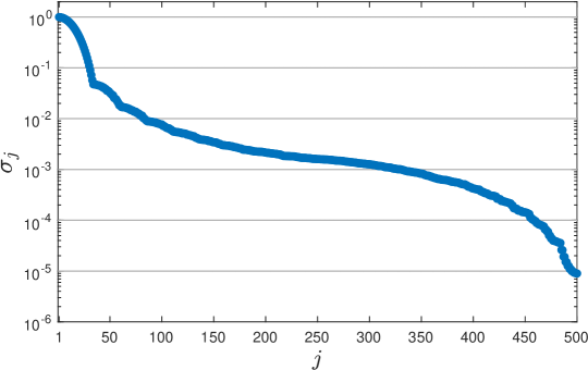
Figure 15: Singular values of the blurring matrix ${\bf A}$ in (8), using the hat function kernel (4) with $n=500$ and $z=0.05$, as used in Figure 8.

Figure 16 shows the right singular vectors associated with the three largest singular values (${\bf v}_{1}$, ${\bf v}_{2}$, and ${\bf v}_{3}$) and the three smallest singular value (${\bf v}_{498}$, ${\bf v}_{499}$, and ${\bf v}_{500}$) of ${\bf A}$.  As expected, the “leading” singular vectors (${\bf v}_{1}$, ${\bf v}_{2}$, ${\bf v}_{3}$) are very smooth, varying little from one entry to the next; they exhibit no fine-scale detail, and are not much affected by blurring. In contrast, the “trailing” singular vectors (${\bf v}_{498}$, ${\bf v}_{499}$, ${\bf v}_{500}$ oscillate quite a bit between entries; they are dominated by fine-scale detail, and blurring will smooth them out almost to zero.

What are the implications of these singular values and vectors for the deblurring operation?

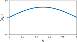
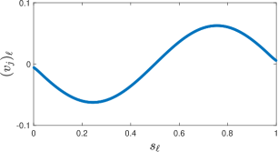
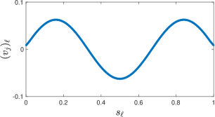
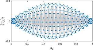
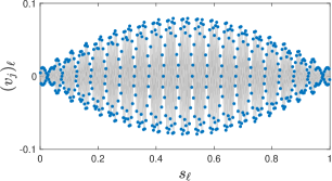
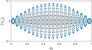
Figure 16: Singular vectors ${\bf v}_{j}$ of the blurring matrix ${\bf A}$ in (8), using the hat function kernel (4) with $n=500$ and $z=0.05$. The singular vectors associated with the largest singular values ($j=1,2,3$) vary quite smoothly from entry to entry, resembling sine waves; these smooth vectors do not change much when blurred. (We have plotted dots for each entry of these vectors, but they appear to be fused into smooth, continuous curves.) In contrast, the singular vectors associated with the smallest singular values ($j=498,499,500$) oscillate quite a bit between entries (highlighted by the gray lines connecting the consecutive values); these vectors have local averages that are quite close to zero.

8.2 Inverting a matrix emphasizes the small singular values

Suppose ${\bf A}\in\mathCR{R}^{n\times n}$ is a square, invertible matrix. Note that ${\bf U},{\bf V}\in\mathCR{R}^{n\times n}$ are square matrices with orthonormal columns, ${\bf U}^{T}{\bf U}={\bf I}$ and ${\bf V}^{T}{\bf V}={\bf I}$, which implies that ${\bf U}^{T}$ and ${\bf V}^{T}$ function as the inverse of a matrix: ${\bf U}^{-1}={\bf U}^{T}$ and ${\bf V}^{-1}={\bf V}^{T}$.  Thus one can write

$${\bf A}{\kern-1.0pt}^{-1}=({\bf U}\mbox{\boldmath$\Sigma$}{\bf V}^{T})^{-1}={\bf V}\mbox{\boldmath$\Sigma$}^{-1}{\bf U}^{T},$$

or in the dyadic form

$${\bf A}{\kern-1.0pt}^{-1}=\sum_{j=1}^{n}{1\over\sigma_{j}}{\bf v}_{j}{\bf u}_{j}^{T}.$$ (20)

This last equation reveals how the singular values of ${\bf A}{\kern-1.0pt}^{-1}$ are the reciprocals (or inverses) of the singular values of ${\bf A}$.  Thus if ${\bf A}$ has very small singular values, ${\bf A}{\kern-1.0pt}^{-1}$ will have some very large singular values. This fact should give us some pause, in light of the observation we made in section 8.1 about the rapidly decaying singular values of blurring matrices! (The idea that “problematic” matrices have large entries in their inverse also arose in the simple $2\times 2$ example in section 4.)

Now apply the formula (20) to solve the system ${\bf A}{\bf f}={\bf b}$ for the unknown vector ${\bf f}$. We find that

$${\bf f}={\bf A}{\kern-1.0pt}^{-1}{\bf b}=\bigg{(}\sum_{j=1}^{n}{1\over\sigma_{j}}{\bf v}_{j}{\bf u}_{j}^{T}\bigg{)}{\bf b}=\sum_{j=1}^{n}{{\bf u}_{j}^{T}{\bf b}\over\sigma_{j}}{\bf v}_{j}.$$ (21)

Here we have distributed the ${\bf b}$ across the sum, and used the fact that ${\bf u}_{j}^{T}{\bf b}\in\mathCR{R}$ is just a scalar value and can thus be moved to the other side of ${\bf v}_{j}$. Equation (21) is crucial to understanding how the inversion process works – or not. It means that

${\bf f}$ can be expressed as a linear combination of the right singular vectors ${\bf v}_{j}$,
and the weight associated with ${\bf v}_{j}$ is given by $({\bf u}_{j}^{T}{\bf b})/\sigma_{j}$.

8.3 Barcodes put more “energy” in larger singular values

What can be said about the coefficients $({\bf u}_{j}^{T}{\bf b})/\sigma_{j}$ for the deblurring examples we have been studying?

First, we note that the blurring matrices ${\bf A}\in\mathCR{R}^{n\times n}$ that we have been considering are symmetric, and have matching right and left singular vectors: ${\bf v}_{j}={\bf u}_{j}$. Thus, the intuition you can draw from Figure 16 about the ${\bf v}_{j}$ vectors also applies to the ${\bf u}_{j}$ vectors.

Since ${\bf A}$ is square, so too is ${\bf U}\in\mathCR{R}^{n\times n}$; recall that the orthonormality of the singular vectors, ${\bf U}^{T}{\bf U}={\bf I}$, means that ${\bf U}^{-1}={\bf U}^{T}$, and hence ${\bf U}{\bf U}^{T}={\bf I}$, too. Thus we can write

$${\bf b}=({\bf U}{\bf U}^{T})\mkern 1.0mu{\bf b}={\bf U}({\bf U}^{T}{\bf b})=\sum_{j=1}^{n}({\bf u}_{j}^{T}{\bf b})\mkern 1.0mu{\bf u}_{j}.$$ (22)

We see that

the coefficient ${\bf u}_{j}^{T}{\bf b}$ reveals the component of ${\bf b}$ in the ${\bf u}_{j}$ direction.

Since the blurred barcodes are relative smooth (see, for example, the plot of ${\bf b}$ in Figure 9), we intuitively expect that smooth ${\bf u}_{j}$ will make the greatest contribution to ${\bf b}$, while rough ${\bf u}_{j}$ will make much smaller contributions. Extrapolating from the six plots of singular vectors shown in Figure 16, we expect ${\bf u}_{j}$ to become increasingly rough as $j$ increases, and thus

we expect $|{\bf u}_{j}^{T}{\bf b}|$ to exhibit, overall, a decreasing trend as $j$ increases.

The left plot in Figure 17 reveals that this is generally the case: for small $j$, $|{\bf u}_{j}^{T}{\bf b}|>1$, while for many larger values of $j$, $|{\bf u}_{j}^{T}{\bf b}|<10^{-6}$. (Notice in particular the sharp drop off that begins around $j=450$.)

The right plot in Figure 17 shows how these coefficients ${\bf u}_{j}^{T}{\bf b}$ change when we divide them by $\sigma_{j}$ in the formula (21) for ${\bf f}={\bf A}{\kern-1.0pt}^{-1}{\bf b}$. Essentially, we are dividing the left plot of Figure 17 by the plot of singular values in Figure 15. In this case, dividing the coefficients ${\bf u}_{j}^{T}{\bf b}$ by the rapidly decaying singular values $\sigma_{j}$ elevates the values of ${\bf u}_{j}^{T}{\bf b}/\sigma_{j}$, most significantly for larger $j$. Indeed, aside from $j=1,\ldots,50$, the value of $|{\bf u}_{j}^{T}{\bf b}|/\sigma_{j}$ is generally around $10^{-2}$. Those larger terms (small $j$) will dominate the sum in (21), in this case by a margin sufficient to make the inversion process stable: ${\bf f}={\bf A}{\kern-1.0pt}^{-1}{\bf b}$ produces a reasonable solution in this case, provided we are using the exact blurring vector ${\bf b}$. What happens when we add a whiff of noise to ${\bf b}$?

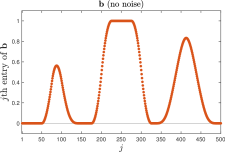
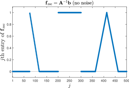
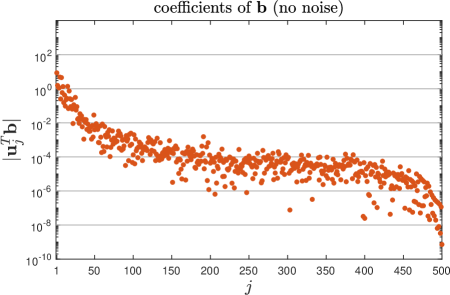
Figure 17: The vectors ${\bf b}$ (top left) and ${\bf f}_{\rm rec}={\bf A}^{-1}{\bf b}$ (top right), with no noise added, along with the magnitude of the coefficients ${\bf u}_{j}^{T}{\bf b}$ for ${\bf b}$ (bottom left) and ${\bf u}_{j}^{T}{\bf b}/\sigma_{j}$ for ${\bf f}_{\rm rec}={\bf A}{\kern-1.0pt}^{-1}{\bf b}$ (bottom right). Notice that ${\bf b}$ has very small components corresponding to the smallest singular values (i.e., large $j$), but these values are lifted much larger in ${\bf f}_{\rm rec}$ due to the division by $\sigma_{j}$. The coefficients for the smoother vector ${\bf b}$ are smaller in magnitude than those for the rougher vector ${\bf f}_{\rm rec}$, for large $j$.

8.4 Random noise scatters “energy” across all singular values

Now let us consider two random “noise” vectors, ${\bf e}_{1}$ and ${\bf e}_{2}$. Both vectors will have normally distributed random entries with mean 0 and standard deviation $10^{-5}\|{\bf b}\|$ (for ${\bf e}_{1}$) and $10^{-3}\|{\bf b}\|$ (for ${\bf e}_{2}$). We can expand these noise vectors in the same way that we expanded ${\bf b}$: for $k=1,2$,

$${\bf e}_{k}=\sum_{j=1}^{n}({\bf u}_{j}^{T}{\bf e}_{k})\mkern 1.0mu{\bf u}_{j}.$$

These vectors ${\bf e}_{1}$ and ${\bf e}_{2}$ are not at all smooth: they vary quite a bit (randomly) from entry to entry. There is no reason why the smooth singular vectors, like ${\bf u}_{1}$ and ${\bf u}_{2}$, should make any greater or lesser contribution to ${\bf e}_{k}$ than the highly oscillatory vectors like ${\bf u}_{n-1}$ and ${\bf u}_{n}$. It is no surprise, then, that their coefficients ${\bf u}_{j}^{T}{\bf e}_{k}$ look nothing like those seen for ${\bf b}$ in Figure 17. Indeed, Figure 18 shows that ${\bf e}_{1}$ (left) and ${\bf e}_{2}$ (right) have roughly the same contributions from most singular vectors ${\bf u}_{j}$; there is no drop-off as $j$ increases.

Since random vectors ${\bf e}_{k}$ exhibit no inherent smoothness,
we expect $|{\bf u}_{j}^{T}{\bf e}_{k}|$ to be roughly the same magnitude for all $j$.
(There should not be any noticeable drop-off as $j$ increases.)

The general order of magnitude of $|{\bf u}_{j}^{T}{\bf e}_{k}|$ is controlled by the noise level: the values in the left plot (noise level $10^{-5}\|{\bf b}\|$) are about $10^{2}$ times smaller than those on the right (noise level $10^{-3}\|{\bf b}\|$).

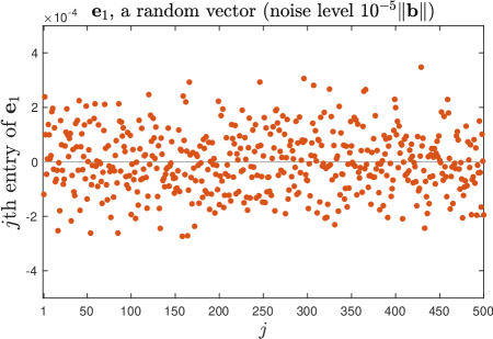
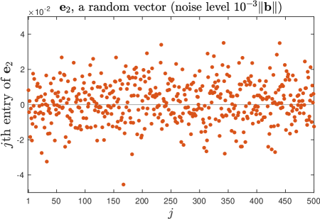
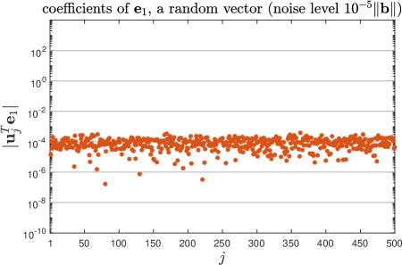
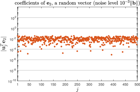
Figure 18: The noise vectors ${\bf e}_{1}$ (top left, noise level $10^{-5}\|{\bf b}\|$) and ${\bf e}_{2}$ (top right, noise level $10^{-3}\|{\bf b}\|$), along with the magnitude of the coefficients ${\bf u}_{j}^{T}{\bf e}_{1}$ for ${\bf e}_{1}$ (bottom left) and ${\bf u}_{j}^{T}{\bf e}_{2}$ for ${\bf e}_{2}$ (bottom right). The noise vectors are not at all smooth. As a result, in contrast to the coefficients for ${\bf b}$ (seen on the left in Figure 17), these coefficients for ${\bf e}_{1}$ and ${\bf e}_{2}$ are fairly uniform across all $j$; no drop-off is seen as $j$ increases.

8.5 Random noise + small singular values = disaster

It is now time to combine the key observations from the last two subsections. We simulate a noisy sample by constructing the vector ${\bf b}_{\rm noise}={\bf b}+{\bf e}_{k}$ for one of the noise vectors ${\bf e}_{1}$ or ${\bf e}_{2}$. When we expand ${\bf b}_{\rm noise}$ in the singular vectors, were merely sum the coefficients from ${\bf b}$ and ${\bf e}_{k}$:

$${\bf b}_{\rm noise}=\sum_{j=1}^{n}\Big{(}{\bf u}_{j}^{T}({\bf b}+{\bf e}_{k})\Big{)}\mkern 1.0mu{\bf u}_{j}=\sum_{j=1}^{n}({\bf u}_{j}^{T}{\bf b})\mkern 1.0mu{\bf u}_{j}+\sum_{j=1}^{n}({\bf u}_{j}^{T}{\bf e}_{k})\mkern 1.0mu{\bf u}_{j}.$$

We are now adding the noise plots from Figure 18 to the coefficients ${\bf u}_{j}^{T}{\bf b}$ from the left plot of Figure 17. The results are shown in Figure 19: For small $j$, the coefficients for ${\bf b}_{\rm noise}$ are dominated by the coefficients ${\bf u}_{j}^{T}{\bf b}$ for ${\bf b}$, until these coefficients decay beneath the noise level seen in Figure 18. Beyond that point, the coefficients ${\bf u}_{j}^{T}{\bf b}_{\rm noise}$ are dominated by the noise contribution ${\bf u}_{j}^{T}{\bf e}_{k}$ for ${\bf e}_{k}$; the rapid drop-off in ${\bf u}_{j}^{T}{\bf b}$ is completely swamped by the noise.

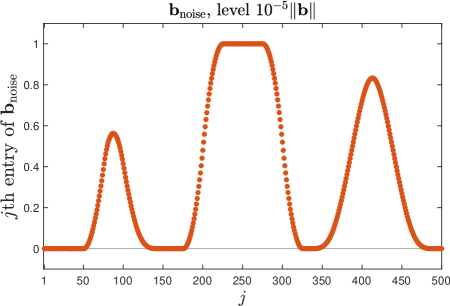
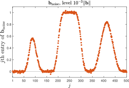
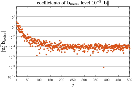
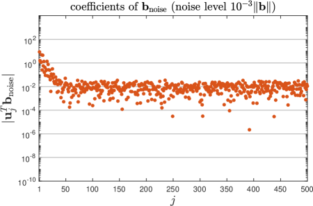
Figure 19: The polluted vectors ${\bf b}_{\rm noise}$ for noise level $10^{-5}\|{\bf b}\|$ (top left) and $10^{-3}\|{\bf b}\|$ (top right), along with the magnitude of the coefficients ${\bf u}_{j}^{T}{\bf b}_{\rm noise}$ below. Compare the left plots to those in Figure 17: even though the $10^{-3}\|{\bf b}\|$ noise is hardly evident in the plot of ${\bf b}_{\rm noise}$, it significantly elevates the coefficients ${\bf u}_{j}^{T}{\bf b}_{\rm noise}$ in the smallest singular values (large $j$). For the larger noise level on the right, these undesirable components are elevated even more.

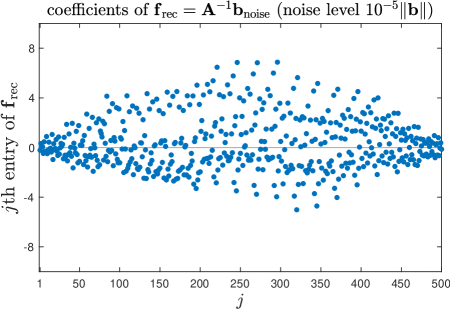
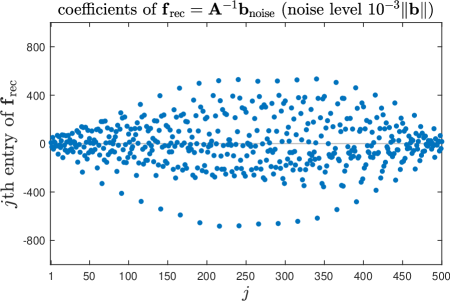
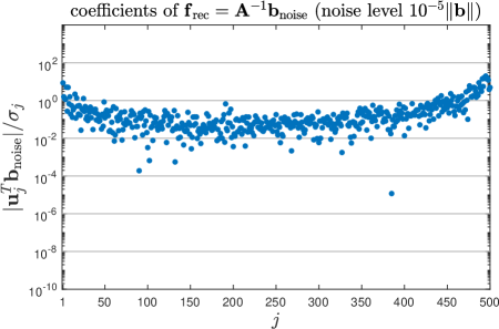
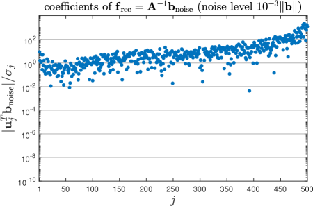
Figure 20: The polluted ${\bf b}_{\rm noise}$ vectors shown in Figure 19 lead to catastrophically poor recovered solutions ${\bf f}_{\rm rec}$, for noise level $10^{-5}\|{\bf b}\|$ (top left) and $10^{-3}\|{\bf b}\|$ (top right). The bottom plots, which show the coefficients $({\bf u}_{j}^{T}{\bf b}_{\rm noise})/\sigma_{j}$ for ${\bf f}_{\rm rec}={\bf A}{\kern-1.0pt}^{-1}{\bf b}_{\rm noise}$, make the problem apparent: For large $j$, moderate values of ${\bf u}_{j}^{T}{\bf b}_{\rm noise}$ are divided by small singular values $\sigma_{j}$, causing these $({\bf u}_{j}^{T}{\bf b}_{\rm noise})/\sigma_{j}$ terms to dominate. The effect is disastrous: the contributions to ${\bf f}_{\rm rec}$ from the trailing singular vectors (e.g., bottom of Figure 16) totally dominate the desirable part of the solution associated with the leading singular vectors (e.g., top of Figure 16).

This perspective exposes the problem that occurs when we compute

$${\bf f}_{\rm rec}={\bf A}{\kern-1.0pt}^{-1}{\bf b}_{\rm noise}=\sum_{j=1}^{n}{{\bf u}_{j}^{T}{\bf b}_{\rm noise}\over\sigma_{j}}\mkern 1.0mu{\bf v}_{j}.$$ (23)

When we divide ${\bf u}_{j}^{T}{\bf b}_{\rm noise}$ by $\sigma_{j}$, we can no longer count on the rapidly decaying values of ${\bf u}_{j}^{T}{\bf b}$ to counteract the rapidly decaying singular values $\sigma_{j}$ (as seen on the right plot in Figure 17).

For small $j$, $\displaystyle{{{\bf u}_{j}^{T}{\bf b}_{\rm noise}\over\sigma_{j}}\approx{{\bf u}_{j}^{T}{\bf b}\over\sigma_{j}}}$, which is accurate.
For large $j$, $\displaystyle{{{\bf u}_{j}^{T}{\bf b}_{\rm noise}\over\sigma_{j}}\approx{{\bf u}_{j}^{T}{\bf e}_{k}\over\sigma_{j}}}$, which is rubbish.

The major problem is, as we can see in Figure 20, the rubbish overwhelms the accurate data. As a result, we will get a nonsense result for ${\bf f}_{\rm rec}={\bf A}{\kern-1.0pt}^{-1}{\bf b}_{\rm noise}$. Take a careful look back on the plots of ${\bf f}_{\rm rec}$ shown in Figure 8 for these two same noise vectors. What shape does ${\bf f}_{\rm rec}$ take? Since the expansion (23) for ${\bf f}_{\rm rec}$ is dominated by $({\bf u}_{j}^{T}{\bf b}_{\rm noise}/\sigma_{j}){\bf v}_{j}$ terms for large values of $j$, it should be no surprise that the computed ${\bf f}_{\rm rec}$ is dominated by shapes that resemble the trailing singular vectors ${\bf v}_{j}$, like those pictured in the bottom half of Figure 16.

When contributions from small singular values (like $\sigma_{n}$) dominate ${\bf f}_{\rm rec}={\bf A}{\kern-1.0pt}^{-1}{\bf b}_{\rm noise}$,
expect ${\bf f}_{\rm rec}$ to resemble the shape of the corresponding singular vectors (like ${\bf v}_{n}$).

8.6 Regularization controls small singular values in the inversion

Now the key problem has been revealed: ${\bf b}_{\rm noise}$ has nontrivial but unwanted components in the most highly oscillatory singular vectors of ${\bf A}$ (i.e., large $j$), and when we compute ${\bf f}_{\rm rec}={\bf A}{\kern-1.0pt}^{-1}{\bf b}_{\rm noise}$ the division by the singular values magnifies those unwanted components to a dominant level. How does regularization fix this issue?

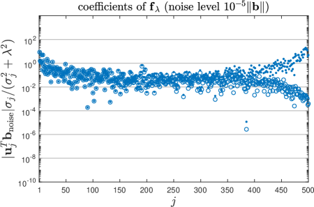
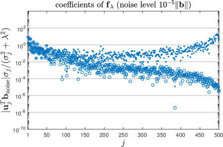
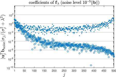
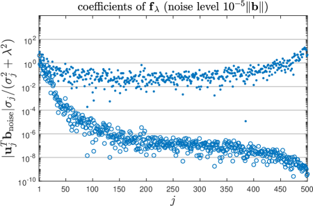
Figure 21: Magnitude of the coefficients of the regularized solution ${\bf f}_{\lambda}$ derived from ${\bf b}_{\rm noise}$ with noise level $10^{-5}\|{\bf b}\|$, for four different values of $\lambda$. (These plots correspond to the bottom four solutions in Figure 11.) The solid dots show $|{\bf u}_{j}^{T}{\bf b}_{\rm noise}|/\sigma_{j}$ for ${\bf f}_{\rm rec}$; the hollow dots show the regularized coefficients $|{\bf u}_{j}^{T}{\bf b}_{\rm noise}|\sigma_{j}/(\sigma_{j}^{2}+\lambda^{2})$. By adjusting $\lambda$ we can dial back the influence of the smaller singular values, but taking $\lambda$ too large will damp out too many terms, thus giving an overly smoothed solution.

To answer that question, we first need to derive an expression for the regularized solution ${\bf f}_{\lambda}$ in the same style as the expansion (23) of ${\bf f}_{\rm rec}$ in the basis of $\{{\bf v}_{j}\}$ vectors. Recall from (15) that we can write

$${\bf f}_{\lambda}=({\bf A}{\kern-1.0pt}^{T}{\bf A}+\lambda^{2}{\bf I})^{-1}{\bf A}{\kern-1.0pt}^{T}{\bf b}.$$

We can use the SVD to reveal additional structure behind this formula. Start at the matrix level with ${\bf A}={\bf U}\mbox{\boldmath$\Sigma$}{\bf V}^{T}$, and recall that orthonormality of the singular vectors ensures ${\bf U}^{T}{\bf U}={\bf I}$ and ${\bf V}{\bf V}^{T}={\bf I}$.  Using these facts we find that

$${\bf A}{\kern-1.0pt}^{T}{\bf A}+\lambda^{2}\mkern 1.0mu{\bf I}\; = \;({\bf U}\mbox{\boldmath$\Sigma$}{\bf V}^{T})^{T}({\bf U}\mbox{\boldmath$\Sigma$}{\bf V}^{T})+\lambda^{2}{\bf I}$$

$$= \;{\bf V}\mbox{\boldmath$\Sigma$}^{T}{\bf U}^{T}{\bf U}\mbox{\boldmath$\Sigma$}{\bf V}^{T}+\lambda^{2}{\bf V}{\bf V}^{T}\ =\ {\bf V}\big{(}\mbox{\boldmath$\Sigma$}^{2}+\lambda^{2}{\bf I}\big{)}{\bf V}^{T},$$

where we have used the fact that $\mbox{\boldmath$\Sigma$}^{T}=\mbox{\boldmath$\Sigma$}$.  Invert this formula to get

$$\big{(}{\bf A}{\kern-1.0pt}^{T}{\bf A}+\lambda^{2}\mkern 1.0mu{\bf I}\big{)}^{-1}\; = \;\Big{(}{\bf V}\big{(}\mbox{\boldmath$\Sigma$}^{2}+\lambda^{2}{\bf I}){\bf V}^{T}\Big{)}^{-1}$$

$$= \;({\bf V}^{T})^{-1}\big{(}\mbox{\boldmath$\Sigma$}^{2}+\lambda^{2}{\bf I}\big{)}^{-1}{\bf V}^{-1}\ =\ {\bf V}\big{(}\mbox{\boldmath$\Sigma$}^{2}+\lambda^{2}{\bf I}\big{)}^{-1}{\bf V}^{T}.$$

Multiply this last expression against ${\bf A}^{T}{\bf b}={\bf V}\mbox{\boldmath$\Sigma$}{\bf U}^{T}{\bf b}$ to arrive at

$${\bf f}_{\lambda}={\bf V}\big{(}\mbox{\boldmath$\Sigma$}^{2}+\lambda^{2}\mkern 1.0mu{\bf I}\big{)}^{-1}\mbox{\boldmath$\Sigma$}\mkern 1.0mu{\bf U}^{T}{\bf b},$$

which can be expressed in terms of the individual singular values and singular vectors, akin to the formula (23) for ${\bf f}_{\rm rec}$, as:

$${\bf f}_{\lambda}=\sum_{j=1}^{n}\bigg{(}({\bf u}_{j}^{T}{\bf b}){\sigma_{j}\over\sigma_{j}^{2}+\lambda^{2}}\bigg{)}{\bf v}_{j}.$$ (24)

Notice the key role that $\lambda>0$ plays in the formula (24) when $\sigma_{j}$ is very small. As $\sigma_{j}\to 0$, observe that $1/\sigma_{j}\to\infty$, (causing blow-up in the formula for ${\bf f}_{\rm rec}$) while $\sigma_{j}/(\sigma_{j}^{2}+\lambda^{2})\to 0$ (avoiding blow-up in the formula for ${\bf f}_{\lambda}$). At the same time, for large values $\sigma_{j}\gg\lambda$, we have $\sigma_{j}/(\sigma_{j}^{2}+\lambda^{2})\approx 1/\sigma_{j}$, and so in this regime $\lambda$ does not interfere much with the solution.

In short, by tuning $\lambda$ correctly we can suppress components of ${\bf f}_{\lambda}$ associated with small singular values, while allowing the desirable components to pass through with little change. Figure 21 clearly illustrates this effect, comparing the coefficients $({\bf u}_{j}^{T}{\bf b}_{\rm noise})/\sigma_{j}$ for ${\bf f}_{\rm rec}$ (solid dots) to the coefficients $({\bf u}_{j}^{T}{\bf b}_{\rm noise})\sigma_{j}/(\sigma_{j}^{2}+\lambda^{2})$ of ${\bf f}_{\lambda}$ (hollow dots), for the same $\lambda$ values used in the bottom four plots of ${\bf f}_{\lambda}$ in Figure 11 (noise level $10^{-5}\|{\bf b}\|$). In all four of these examples, the ‘tail’ of elevated coefficients for ${\bf f}_{\rm rec}$ seen in the left plot of Figure 20 is suppressed by regularization, to an increasing degree as $\lambda$ grows. In Figure 21 we saw that the three values $\lambda=10^{-3}$, $10^{-2}$, and $10^{-1}$ give reasonable solutions that increase in smoothness, consistent with the more aggressive suppression of ${\bf v}_{j}$ for large $j$ due to the $\sigma_{j}/(\sigma_{j}^{2}+\lambda^{2})$ term. Taking $\lambda=10^{0}$ suppresses too many terms, leading to an unacceptably smoothed solution.

This section has illustrated how the singular value decomposition can illuminate the regularization process. Indeed, it is a remarkable tool for analyzing the solution of linear systems, least squares problems, low-rank approximation and dimension reduction, and many other rich applications. In the same way, the simple deblurring example described in this manuscript is but a taste of the rich and vital world of inverse problems, with applications that range from image deblurring to radar, from landmine detection to ultrasound. Many avenues remain for your exploration!

Questions for Reflection

• It might seem like a leap to move from the product-of-matrices form of the SVD in (17) and the dyadic form (19). Consider the following $2\times 2$ matrices

  $${\bf U}=\left[\begin{array}[]{cc}{\bf u}_{1}&{\bf u}_{2}\end{array}\right]=\left[\begin{array}[]{cc}u_{1,1}&u_{2,1}\\ u_{1,2}&u_{2,2}\end{array}\right],\qquad{\bf V}=\left[\begin{array}[]{cc}{\bf v}_{1}&{\bf v}_{2}\end{array}\right]=\left[\begin{array}[]{cc}v_{1,1}&v_{2,1}\\ v_{1,2}&v_{2,2}\end{array}\right],$$

  where, e.g., $u_{j,k}$ refers to the $k$th entry of the vector ${\bf u}_{j}$.

  By multiplying each expression out, entry-by-entry, show that ${\bf U}{\bf V}^{T}={\bf u}_{1}{\bf v}_{1}^{T}+{\bf u}_{2}{\bf v}_{2}^{T}$.

• Think back to the local averaging kernel (3). Can you design a function $f(t)$ such the blurred function

  $$b(s)=\int_{0}^{1}h(s,t)f(t)\,{\rm d}t$$

  is close to zero for all $s\in[0,1]$? How would such a function relate to the singular vectors of the discretization matrix ${\bf A}$ for this blurring kernel?

Now would be a good time to explore Exercises E8.1–E8.3 starting on page E8.1.

 

Exercises

• Experiment with the blurring operation as shown in Figure 6. You can generate the function $f$ using the code below.

  ⬇

  def f_function(t=0.5):

  f1 = (t>=0.15)*np.maximum(1-12*(t-.15),0) # a down ramp

  f2 = np.abs(t-0.5)<=.1 # a step

  f3 = np.maximum(1-10*np.abs(t-0.825),0) # a hat

  return f1+f2+f3

  For $n=100$, you can create a vector ${\bf f}$, blurring matrix ${\bf A}$, and blurred vector ${\bf b}={\bf A}{\bf f}$ using the code below. Note that build_blur_A uses the Gaussian blurring kernel, here called with parameter $z=0.025$.

  ⬇

  n = 100

  z = 0.025

  t = np.array([(k+.5)/n for k in range(n)]) # t_k points

  f = f_function(t) # evaluate f(t_k)

  A = build_blur_A(n,z) # build blurring matrix

  b = A@f # b=A*f (matrix times vector)

  You can then plot the entries of ${\bf f}$ and ${\bf b}$ as dots using the following commands.

  ⬇

  import matplotlib.pyplot as plt

  plt.plot(t,f_function(t),’.’,markersize=5,label=’f’)

  plt.plot(t,b,’.’,markersize=5,label=’b’)

  plt.legend()

  Execute these commands to produce your own plot of ${\bf f}$ and ${\bf b}$. (Your plot will differ slightly from the one shown in Figure 6, which uses the local averaging blurring kernel (3), whereas the code above uses the Gaussian kernel (5).)

  Now experiment with the value of $z$, the dimension $n$, and the choice of blurring kernel. (As you change these parameters, be sure to regenerate your ${\bf A}$ matrix.) Produce plots to show how these parameters affect the blurring operation.

• The code in Figure 5 built the blurring matrix ${\bf A}$ by row. What if instead we followed the more natural approach of building ${\bf A}$ by entry? The code is given below.

  ⬇

  def build_blur_A_by_entry(n=100,z=.025):

  A = np.zeros((n,n)); # n-by-n matrix of zeros

  s = np.array([(j+.5)/n for j in range(n)]) # s_j points

  t = np.array([(k+.5)/n for k in range(n)]) # t_k points

  for j in range(0,n):

  for k in range(0,n):

  A[j,k] = h_gaussian(s[j],t[k],z)/n # A(j,k) = h(s_j,t_k)/n

  return A

  This problem explores if there is an efficiency advantage to building ${\bf A}$ by row. You can time a command in Python by adjusting the following template.

  ⬇

  import time

  t0 = time.time() # start timer

  # insert the commands you want to time here

  elapsed_time = time.time() - t0 # show elapsed time

  • Compute the time it takes to build the $n=1000$ blurring matrix ${\bf A}$ by row (use the code build_blur_A from Figure 5).

  • Repeat the same timing (be sure to reset t0 = time.time()), but now building ${\bf A}$ entry-by-entry (use the code build_blur_A_by_entry given above). How does the time compare?

  • Repeat (a) and (b) with $n=1000$. How do the timings change when the dimension $n$ doubles from $500$ to $1000$? Can you explain why the timing grows like this?

  • Modify build_blur_A to build ${\bf A}$ one column at a time. How does the timing of this routine compare to the timing for the the row-oriented and entry-by-entry methods?

   

• In problem E2.1 you blurred a signal ${\bf f}$ to get ${\bf b}={\bf A}{\bf f}$, where ${\bf A}$ uses the Gaussian blurring function (5) with $n=100$ and $z=0.025$.

  Replicate the experiment shown in Figure 7 using this Gaussian kernel. Following the example in the code below, add random noise of level $10^{-3}\|{\bf b}\|$ to ${\bf b}$ to get ${\bf b}_{\rm noise}$. Then solve for ${\bf f}_{\rm rec}={\bf A}{\kern-1.0pt}^{-1}{\bf b}_{\rm noise}$ using the np.linalg.solve command in Python. (This approach uses Gaussian elimination to solve $A{\bf f}_{\rm rec}={\bf b}_{\rm noise}$ for the unknown vector ${\bf f}_{\rm rec}$, which is preferable to computing ${\bf A}{\kern-1.0pt}^{-1}$ and multiplying the result against ${\bf b}_{\rm noise}$ to get ${\bf f}_{\rm rec}$.)

  ⬇

  n = 100

  z = 0.025;

  eps = 0.001;

  t = np.array([(k+.5)/n for k in range(n)])

  A = build_blur_A(n,z)

  f = f_function(t) # compute the true signal

  b = A@f # blur the true signal

  s = eps*np.linalg.norm(b) # standard deviation of noise

  e = s*np.random.randn(n) # generate random noise

  bnoise = b+e # simulate a noisy observation

  frec = np.linalg.solve(A,bnoise) # solve A*frec=bnoise for frec

  plt.plot(t,f,’.’,color=’blue’,markersize=5,label=’$f$’)

  plt.plot(t,frec,’.’,markerfacecolor=’none’,color=’blue’,\

  markersize=8,label=’$f_{rec}$’)

  plt.legend()

• Repeat Exercise E3.1, but reduce the noise level down to $10^{-5}\|{\bf b}\|$, $10^{-7}\|{\bf b}\|$, and $10^{-9}\|{\bf b}\|$. Does ${\bf f}_{\rm rec}$ improve as the level of noise drops?

• Now take $n=500$, still with $z=0.025$. This larger value of $n$ should mean that our blurring operation incurs less discretization error when we convert the calculus problem into a linear algebra problem. You might speculate this extra accuracy in the approximation of the blurring integral would lead to a better recovered value for ${\bf f}_{\rm rec}$. This question explores whether this conjecture is accurate. We want to determine how increasing $n$ affects the accuracy of the recovered signal.

  Repeat Exercise E3.1 with $n=500$ and noise level $10^{-3}\|{\bf b}\|$. Is ${\bf f}_{\rm rec}$ accurate?

  What if we attempt to compute ${\bf f}_{\rm rec}$ directly from ${\bf b}$, with no artificial noise added (i.e., bnoise=b). Does frec = np.linalg.solve(A,b) produce the correct ${\bf f}$?

   

• Suppose we redefine ${\bf A}$ so that it depends on a parameter $\alpha>0$:

  $${\bf A}=\left[\begin{array}[]{cc}1&-\alpha\\ 1&\phantom{-}\alpha\end{array}\right].$$

  1. Compute a formula for ${\bf A}{\kern-1.0pt}^{-1}$, which will depend upon $\alpha$.

     How does ${\bf A}{\kern-1.0pt}^{-1}$ change as $\alpha\to 0$?

  2. Using your formula from part (a), write out ${\bf A}{\kern-1.0pt}^{-1}$ for the specific value $\alpha=0.001$.

  3. Again with $\alpha=0.001$, suppose

     $${\bf b}_{1}=\left[\begin{array}[]{c}1\\ 1\end{array}\right],\qquad{\bf b}_{2}=\left[\begin{array}[]{c}1\\ 1.01\end{array}\right].$$

     Solve for ${\bf f}_{1}={\bf A}{\kern-1.0pt}^{-1}{\bf b}_{1}$ and ${\bf f}_{2}={\bf A}{\kern-1.0pt}^{-1}{\bf b}_{2}$.

     How does the difference between the solutions, $\|{\bf f}_{2}-{\bf f}_{1}\|$, compare to the difference between the data, $\|{\bf b}_{2}-{\bf b}_{1}\|$?

   

• This exercise investigates the connection between the objective function (10) and the least squares problem (16).

  1. For any vectors ${\bf x},{\bf y}\in\mathCR{R}^{n}$, show that

     $$\left\|\left[\begin{array}[]{c}{\bf x}\\ {\bf y}\end{array}\right]\right\|^{2}=\|{\bf x}\|^{2}+\|{\bf y}\|^{2}.$$

  2. Now show that

     $$\left\|\left[\begin{array}[]{c}{\bf b}\\ {\bf 0}\end{array}\right]-\left[\begin{array}[]{c}{\bf A}\\ \lambda\mkern 1.0mu{\bf I}\end{array}\right]\mkern 1.0mu{\bf f}\,\right\|^{2}=\|{\bf b}-{\bf A}{\bf f}\|^{2}+\lambda^{2}\mkern 1.0mu\|{\bf f}\|^{2},$$

     and explain why $\phi({\bf f})$ in (10) is thus minimized by the same ${\bf f}$ that solves the least squares problem (16).

• Suppose that

  $${\bf A}=\left[\begin{array}[]{ll}1&1\\ 1+10^{-6}&1-10^{-6}\end{array}\right],\qquad{\bf b}=\left[\begin{array}[]{l}1\\ 1\end{array}\right].$$

  Set $\lambda=10^{-8}$. Solve for ${\bf f}_{\lambda}$ using (10) using Gaussian elimination (e.g., via the np.linalg.solve command), and by solving the least squares problem (16) (e.g., via the np.linalg.lstsq command). Show your results to at least 8 decimal places. Do your answers agree? If not, which one do you think is more accurate? Why?

   

• Using the code above as a starting point, generate an L curve like the one shown in Figure 13 by taking the following steps.

  1. Reproduce Figure 13 using the same parameters: take $n=500$, generate ${\bf A}$ to use the hat-function blurring kernel 4 with $z=0.05$, and set the noise level to be $10^{-5}\|{\bf b}\|$.

  2. Compute the regularized solutions for several special values of $\lambda$; on top of your L curve plot from part (a), plot $(\|{\bf b}_{\rm noise}-{\bf A}{\bf f}_{\lambda}\|,\|{\bf f}_{\lambda}\|)$ as red circles.

  3. Adapt your code to use the Gaussian kernel 5 with $z=0.01$ and noise level $10^{-5}\|{\bf b}\|$. Adjust the blurring parameter $z$ and/or the noise level, and see how these changes affect the L curve plot.

     Note: as you adjust the parameters in your model, you might need to change the range of $\lambda$ values you are using (defined in lamvec); it is also a good idea to remove the lines that set the axis limits (plt.xlim and plt.ylim), as the location of the L curve will change as you adjust the problem.

   

• Using the unpolluted blurred vector ${\bf b}$, produce a plot showing the vector ${\bf f}_{\rm rec}$ one obtains by directly solving ${\bf A}{\bf f}_{\rm rec}={\bf b}$ (e.g., frec = numpy.linalg.solve(A,b)) via Gaussian elimination. To produce an elongated plot like the ones shown above in Python, you can adapt the following code.

  ⬇

  plt.figure(figsize=(10,1.85)) % create an elongated figure window

  plt.plot(t,f,’b.’) % plot f_true

  plt.xlabel(’$s_j$’,fontsize=14) % label horizontal axis s_j

  plt.ylabel(’$f_j$’,fontsize=14) % label vertical axis f_j

  plt.tight_layout()

• Now using the polluted vector ${\bf b}_{\rm noise}$, repeat the last exercise: use Gaussian elimination (numpy.linalg.solve) to solve ${\bf A}{\bf f}_{\rm noise}={\bf b}_{\rm noise}$ for ${\bf f}_{\rm noise}$. Plot your recovered barcode ${\bf f}_{\rm noise}$. Does your solution at all resemble ${\bf f}_{\rm true}$?

• Explore the solutions obtained from the regularized least squares problem

  $$\min_{{\bf f}\in\mathCR{R}^{n}}\|{\bf A}{\bf f}-{\bf b}\|^{2}+\lambda^{2}\|{\bf f}\|^{2}$$

  for various values of $\lambda>0$. Recall from Section 5 that you can find ${\bf f}_{\lambda}$ by solving the least squares problem

  $$\min_{{\bf f}\in\mathCR{R}^{n}}\|\widehat{{\bf b}}-{\bf A}_{\lambda}{\bf f}\|,$$

  where

  $${\bf A}_{\lambda}=\left[\begin{array}[]{c}{\bf A}\\ \lambda{\bf I}\end{array}\right]\in\mathCR{R}^{2n\times n},\qquad\widehat{{\bf b}}=\left[\begin{array}[]{c}{\bf b}\\ {\bf 0}\end{array}\right]\in\mathCR{R}^{2n}.$$

  This least squares problem can be solved in Python via the np.linalg.lstsq command.

  1. Using the value ${\bf b}_{\rm noise}$ (be sure to use ${\bf b}_{\rm noise}$), create an L curve plot using parameter values $\lambda=10^{-6},\ldots,10^{1}$. (Use lam = np.logspace(-6,1,100) to generate 100 logarithmically-spaced values of $\lambda$ in this range.) Recall that the L curve is a plt.loglog plot with $\|{\bf b}_{\rm noise}-{\bf A}{\bf f}_{\lambda}\|$ on the horizontal axis and $\|{\bf f}_{\lambda}\|$ on the vertical axis. (Be sure you are using ${\bf b}_{\rm noise}$ to compute the norm of the misfit for the horizontal axis, $\|{\bf b}_{\rm noise}-{\bf A}{\bf f}_{\lambda}\|$.)

  2. Pick several $\lambda$ values corresponding to the main corner in the L-curve (or just a bit beyond this point), solve for the regularized solution ${\bf f}_{\lambda}$, and plot ${\bf f}_{\lambda}$. Show plots for a few different $\lambda$ values that vary over several orders of magnitude. Also show the ${\bf f}_{\lambda}$ you get for the same value of $\lambda$ if you instead use the true data ${\bf b}$ instead of ${\bf b}_{\rm noise}$.

• Using your best recovered ${\bf f}_{\lambda}$ from Exercise E7.3, reconstruct the barcode for the can of Coke. (You should decode the specific numbers shown at the bottom of the Coke barcode presented earlier; it is not enough to just recover the function $f$ itself.) This is a little tricky – do your best, using insight from the structure of the UPC code function to help.

• Edit the coke_upc function to create bnoise with more noise, such as $5\times 10^{-3}\|{\bf b}\|$ (instead of the $10^{-3}\|{\bf b}\|$ in the original coke_upc code). Can you still reliably compute the barcode? If so, how much more noise can you add, before it becomes very difficult to recover the correct bar code (even with the use of regularization)?

• The file mystery_bnoise1.csv specifies the blurred, noisy ${\bf b}_{\rm noise}$ barcode for a mystery product (again with n=570 and the same ${\bf A}$ as for the Coke barcode).

  You can load the file with the simple command

  ⬇

  bnoise = np.loadtxt(’mystery_bnoise1.csv’)

  1. Use the techniques from Exercise E7.3 to attempt to recover the function $f$ associated with the mystery barcode. Show samples of the results from your various attempts.

  2. Decode the UPC from your best recovered solution ${\bf f}_{\lambda}$ from part (a). (Be sure to explain your process.) What is the product described by the mystery UPC? (Once you have found the correct UPC, a search on Amazon or https://www.barcodelookup.com should turn up the product.)

• Repeat the deblurring process for the blurred barcode stored in mystery_bnoise2.csv, which is a bit noisier that the previous mystery UPC (but again uses n=570 and the same ${\bf A}$ as for the two previous barcodes).

  To what product does this blurry barcode correspond? Include your evidence.

   

• Compute the singular values of the blurring matrix (8) for the Gaussian kernel (5) with $n=570$ and $z=0.01$, as used in the barcode decoding experiments in the exercises at the end of section 7. How does the decay of the singular values for this kernel compare with what we observed for the hat function kernel in Figure 15? What insight does your plot give you about the sensitivity of the UPC deblurring operation?

• Repeat the experiments in this section for the Coke UPC decoding example described earlier, blurring with the Gaussian kernel as in the last problem. Compare the results you obtain using the unpolluted vector ${\bf b}$, as well as ${\bf b}_{\rm noise}$ with different levels of noise.

• The discussion in this section might cause you to ask: if small singular values cause problems in the formula (23) for ${\bf f}_{\rm rec}$, why not just chop those troublesome terms off of the sum, stopping after $k<n$ terms:

  $${\bf f}_{k}=\sum_{j=1}^{k}{{\bf u}_{j}^{T}{\bf b}_{\rm noise}\over\sigma_{j}}\mkern 1.0mu{\bf v}_{j}.$$ (25)

  This truncated SVD solution can be a very effective alternative to the regularization method presented in this manuscript.

  Repeat the Coke UPC decoding operation using the truncated SVD solution ${\bf f}_{k}$. Can you correctly decode the UPC from ${\bf f}_{k}$? Try a range of $k$ values. Which $k$ values give smoother or rougher solutions?

Modeling Projects

1. Find a UPC barcode for some product of your choice. Make your own version of Exercises E7.6 and E7.7. Turn your barcode in an ${\bf f}$ vector. Apply the blur, ${\bf b}={\bf A}{\bf f}$, add some noise to get ${\bf b}_{\rm noise}$, and then give the result to a friend to decode.

2. All our barcode deblurring work has been based on taking $n=570$, which means that each of the 95 units that make up a barcode is discretized with 6 entries in the vector ${\bf f}\in\mathCR{R}^{570}$ (notice that $95\times 6=570$).

   What if you rework everything using only 2 entries per unit (giving ${\bf b},{\bf f}\in\mathCR{R}^{190}$ and ${\bf A}\in\mathCR{R}^{190\times 190}$). Reducing the size of the matrices and vectors will make the linear algebra faster. Does it make the barcode deblurring easier or harder? Show evidence.

   What if you rework everything using 10 entries per unit (giving ${\bf b},{\bf f}\in\mathCR{R}^{950}$ and ${\bf A}\in\mathCR{R}^{950\times 950}$). Enlarging the size of the matrices and vectors will make the linear algebra slower. Does it make the barcode deblurring easier or harder? Show evidence.

3. The previous modeling project asks you to experiment with blurring matrices of different dimension. Increasing $n$ leads to a more high-fidelity model, with a more accurate approximation to the blurring integral (7).

   Construct the blurring matrix ${\bf A}$ in (8), using the hat function kernel (4) with $z=0.05$, but now with $n=1000$. Compute the singular values, and compare them to those shown for $n=500$ in Figure 15. What happens to the smallest singular values?

   Repeat the experiments of Section 8 with $n=1000$. Is the recovered solution ${\bf f}_{\rm rec}={\bf A}^{-1}{\bf b}_{\rm noise}$ more or less susceptible to noise in ${\bf b}_{\rm noise}$, compared to the $n=500$ case? Use regularization to compute ${\bf f}_{\lambda}$ for several $\lambda$ values. Does regularization work?

   Now repeat these experiments with $n=2000$ (or larger). Can you deduce a trend in performance as $n$ increases?

4. The “images” we have deblurred in this manuscript have all been one-dimensional. Such primitive “images” make the modeling a bit clearer to explain, but are perhaps less satisfying to study than true two-dimensional images. Two dimensions requires two independent variables, and so the true image becomes $f(t^{(1)},t^{(2)})$, with its blurry counterpart $b(s^{(1)},s^{(2)})$. The analog of the blurring operation (2) takes the form

   $$b(s^{(1)},s^{(2)})=\int_{0}^{1}\int_{0}^{1}h\left(\left[\!\begin{array}[]{c}s^{(1)}\\ s^{(2)}\end{array}\!\right],\left[\!\begin{array}[]{c}t^{(1)}\\ t^{(2)}\end{array}\!\right]\right)f(t^{(1)},t^{(2)})\,{\rm d}t^{(1)}{\rm d}t^{(2)}.$$ (26)

   1. Generalize one of the blurring functions (3), (4), and (5) to obtain a suitable $h$ for this two dimensional setting.

   2. Discretize $s^{(1)},s^{(2)}\in[0,1]$ into $n$ points $s_{\ell}=(\ell-1/2)/n$ for $\ell=1,\ldots,n$, and approximate the double integral (26) with a double sum:

      $$b(s_{\ell},s_{m})\approx b_{\ell,m}=\frac{1}{n^{2}}\sum_{j=1}^{n}\sum_{k=1}^{n}h\left(\left[\!\!\begin{array}[]{c}s_{\ell}\\ s_{m}\end{array}\!\!\right],\left[\!\begin{array}[]{c}t_{j}\\ t_{k}\end{array}\!\right]\right),$$ (27)

      where $t_{j}=(j-1/2)/n$.

      Explain how to arrange the equation (27) for $\ell,m=1,\ldots,n$ into the form of a linear system ${\bf b}={\bf A}{\bf f}$, where ${\bf A}\in\mathCR{R}^{n^{2}\times n^{2}}$ and

      $${\bf b} = [\begin{array}[]{ccccccc}b_{1,1}&\cdots&b_{n,1}&\cdots&b_{1,n}&\cdots&b_{n,n}\end{array}]^{T}\in\mathCR{R}^{n^{2}\times 1}$$

      $${\bf f} = [\begin{array}[]{ccccccc}f(t_{1},t_{1})&\cdots&f(t_{n},t_{1})&\cdots&f(t_{1},t_{n})&\cdots&f(t_{n},t_{n})\end{array}]^{T}\in\mathCR{R}^{n^{2}\times 1}.$$

      To make things concrete, write everything out for the case $n=3$.

   3. Find a grayscale image, and use an image editing program to adjust its size to $n\times n$ pixels, for some modest value of $n$. Take $f(t_{j},t_{k})$ to be the value of the $(j,k)$ pixel, so that, for a grayscale image, $f(t_{j},t_{k})$ will be an integer between 0 (black) and 255 (white). Plot the image as a heat map.

   4. Code up the matrix ${\bf A}$ in part (b) for a general value of $n$, Take your $f$ from part (c), and reshape it into the vector ${\bf f}\in\mathCR{R}^{n^{2}\times 1}$. Blur the image: ${\bf b}={\bf A}{\bf f}$. Reshape ${\bf b}$ into an $n\times n$ matrix, and visualize the result as a heat map.

   5. Attempt to deblur the image by solving ${\bf f}_{\rm rec}={\bf A}^{-1}{\bf b}$. How does the process perform? What if noise is added to ${\bf b}$? Explore the use of regularization to stabilize the deblurring process.

   Note: When working with two dimensional images, the linear algebra becomes quite a bit more expensive. (For example, if $n=1000$, then $n^{2}=10^{6}$, and your ${\bf A}$ would be a million-by-a million matrix.) For these experiments, try using $n=40$ or $n=60$.

   For more details about the two-dimensional blurring process in the spirit of this manuscript (and hints for some of the above problems), see [1, Section 8.3].

Bibliography

- [1] M. Embree, Matrix Methods for Computational Modeling and Data Analytics. Available at: https://personal.math.vt.edu/embree/cmda3606notes.pdf, 2023.
- [2] G. H. Golub and C. F. Van Loan, Matrix Computations, Johns Hopkins University Press, Baltimore, fourth ed., 2012.
- [3] GS1, GS1 General Specifications Standard, January 2023, https://ref.gs1.org/standards/genspecs/.
- [4] A. L. Haberman (Ed.), Twenty-five Years Behind Bars: The Proceedings of the Twenty-fifth Anniversary of the UPC at the Smithsonian Institution, September 30, 1999, Harvard University Press, Cambridge, MA, 2001.
- [5] P. C. Hansen, Discrete Inverse Problems: Insight and Algorithms, SIAM, Philadelphia, 2010.
- [6] M. A. Iwen, F. Santosa, and R. Ward, A symbol-based algorithm for decoding barcodes, SIAM J. Imaging Sci., 6 (2013), pp. 56–77.
- [7] R. Mars, Barcodes, 99% Invisible, (2014), https://99percentinvisible.org/episode/barcodes/. Audio podcast episode.
- [8] F. Santosa and M. Goh, Bar code decoding in a camera-based scanner: analysis and algorithm, SIAM J. Imaging Sci., 15 (2022), pp. 1017–1040.
- [9] G. Strang, Introduction to Linear Algebra, Wellesley-Cambridge, Wellesley, MA, sixth ed., 2023.
- [10] E. Süli and D. Mayers, An Introduction to Numerical Analysis, Cambridge University Press, Cambridge, 2003.
- [11] T. Whittman, Lost in the supermarket: Decoding blurry barcodes, SIAM News, 37 (September, 2004).
- [12] Wikipedia contributors, Universal product code – Wikipedia, the free encyclopedia, 2023, https://en.wikipedia.org/wiki/Universal_Product_Code. [Online; accessed 19-June-2023].