Core Collapse Beyond the Fluid Approximation: The Late Evolution of Self-Interacting Dark Matter Halos

Abstract

We show that the gravothermal collapse of self-interacting dark matter (SIDM) halos can deviate from local thermodynamic equilibrium. As a consequence, the self-similar evolution predicted by the commonly adopted conducting fluid model can be altered or broken. Our results are obtained using a novel, efficient kinetic solver called KiSS-SIDM for tracing the gravothermal evolution based on the Direct Simulation Monte Carlo (DSMC) framework. In the long mean free path stage, the code is a viable alternative to the fluid model, yet requires no calibration parameters. Further, this method enables a fully kinetic treatment well into the late, short mean free path, stage of the collapse. We apply the method to a canonical case with isotropic, velocity independent scattering. We find that although a fluid treatment is appropriate deep in the short mean free path core, departures from local thermodynamic equilibrium develop in the intermediate mean free path region bounding the core, which modify the late-time evolution.

I Introduction

Despite decades of research, the particle nature of dark matter (DM) remains unknown. In one class of models, (some of) the DM possesses an elastic scattering self-interaction, which is referred to as self-interacting dark matter (SIDM). This scattering transports thermal energy in SIDM halos. Initially, the energy transport thermalizes the DM in the center of the halo, leading to the formation of a core. Eventually, the outward energy transport from the hot core to the cool envelope of the halo leads to a runaway collapse, the “gravothermal catastrophe”. This basic physical picture has been invoked to explain numerous astrophysical observations, including the diversity of galactic rotation curves and the formation of massive quasars at high redshift [3, 14, 8, 13]. However, obtaining a quantitative handle on the late evolutionary stages has proved challenging, and the endpoints of the collapse remain poorly understood. This is because the dynamics are described by the collisional Boltzmann equation, which is a formidable challenge for numerical methods due to the six-dimensional phase space.

Practically, computational approaches to this problem have bifurcated. When the mean free path (MFP) is long compared to the gravitational scale height (the LMFP regime), existing $N$-body codes have been modified to allow pairwise scattering between nearby particles [5, 15, 28, 26, 31]. This method becomes prohibitively expensive as the density increases and the MFP becomes short, because it requires identifying and calculating pairwise scattering probabilities between all nearby particles at each time step. Moreover, extensive recent research has emphasized the challenges of obtaining converged results and conserving the total energy of the system through the collapse [24, 9, 18, 19].

Meanwhile, in the short mean free path (SMFP) limit, the behavior of the DM is treated by a moment approach to the Boltzmann equation, closed via an ideal gas equation of state and an effective thermal conductivity. This “conducting fluid” (e. g. [3, 7, 21, 23, 10]) model has been adopted in the SMFP regime where the thermal conductivity can be derived from first principles [6]. If the thermal conductivity is appropriately calibrated, the fluid approach can also produce good agreement with $N$-body simulations in the LMFP limit, at reduced computational cost. Recent work [33, 17] has focused on the details of this calibration procedure. However, the assumptions of the model have not been evaluated in the short and intermediate MFP regimes. Especially, the intermediate regime (where the MFP is comparable to the gravitational scale height) is problematic both for the fluid model and for $N$-body codes. In the former, an ad-hoc interpolation in the conductivity must be adopted, while in the latter the computational cost already becomes very high.

II Methods

A standard technique in the computational fluid dynamics literature for approximate numerical solutions to the collisional Boltzmann equation is the Direct Simulation Monte Carlo (DSMC, [4, 22, 25]) algorithm. As in astrophysical $N$-body codes, a finite number of discrete tracers are used to sample the continuous distribution function, and elastic collisions are simulated between pairs of tracer particles. However, in the DSMC approach simulation particles are grouped into cells whose length is required to be smaller than the MFP. Scattering is allowed only between particles within the same cell. In the “majorant collision frequency” scheme which we adopt, at each time step and in each cell an upper bound on the number of collisions, $\Gamma_{i}$ is calculated. Then, for $\Gamma_{i}$ randomly chosen pairs of particles a rejection sampling is performed to determine if a collision occurs.

This approach enjoys several advantages compared to the standard neighbor search implementation in $N$-body codes. First, the cell to which each particle belongs can be stored and dynamically updated, obviating the neighbor search step. Second, it is guaranteed that no scattering will occur between particles separated by more than one MFP. Finally, the number of trial collisions decreases in proportion to the timestep, which greatly reduces the overhead of adopting a timestep much smaller than the scattering timescale. This allows us to adopt a global (rather than per particle) time step, substantially improving the energy accuracy [9].

In our implementation, we assume spherical symmetry: all particles in the same spherical shell are allowed to scatter off of each other regardless of their angular coordinates. Therefore, the distribution function in each radial bin is extremely well resolved compared to a fully three-dimensional simulation with the same parameters and particle number. We likewise exploit this symmetry in calculating the gravitational acceleration.

We defer extensive discussion of the validation and convergence tests we have performed to separate work. More details about the code, which we call KiSS-SIDM (“Kinetic Spherically Symmetric SIDM”), are provided in the End Matter. We have checked that KiSS-SIDM reproduces the SMFP Chapman–Enskog thermal conductivity to within $2\text{\,}\mathrm{\char 37\relax}$. The energy is conserved in the fiducial halo case discussed below to $|\Delta E/E|<$2\text{\times}{10}^{-4}$$. The method is computationally inexpensive in the short and intermediate MFP regimes: the core formation and early collapse results are converged with $\sim 10^{5}$ particles, an order of magnitude fewer than in [18], and require roughly 30 minutes on a laptop.

III Results

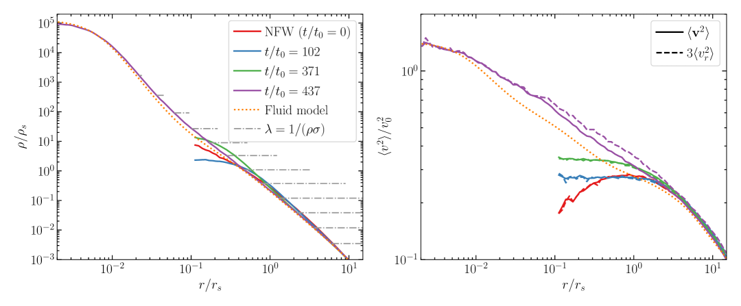
Figure 1: Left: The density profiles in the simulation at different times (solid) and at a matched central density (at the final time) in the fluid model (dotted). The MFP at different densities is also plotted (length of the dashed lines). Right: The velocity dispersion profiles for the same cases, 3D (solid) and triple the radial velocity dispersion (dashed). In the fluid model, the velocity dispersion is isotropic.

We simulate an initially Navarro–Frenk–White (NFW) halo [20] consisting of $2\text{\times}{10}^{6}$ particles. A constant cross section large enough to collapse the core of typical galaxy-sized halos within the age of the universe is likely excluded by observations [1]. However, studies which consider the presence of baryons [8], tidal stripping [21], or a velocity-dependent cross section [32] find runaway collapse by the present day. Here, we examine the canonical case of a constant cross section in an NFW halo in order to clearly illustrate the physics of the gravothermal collapse. Specifically, the density profile is:

$$\rho(r)=\frac{\rho_{\mathrm{s}}}{\left(1+\frac{r}{r_{\mathrm{s}}}\right)^{2}\left(\frac{r}{r_{\mathrm{s}}}\right)},$$ (1)

with $\rho_{\mathrm{s}}$ the scale density and $r_{\mathrm{s}}$ the scale radius. From the scale radius and density we define $M_{0}=r_{\mathrm{s}}^{3}\rho_{\mathrm{s}}$, $v_{0}=\sqrt{GM_{0}/r_{\mathrm{s}}}$, $t_{0}^{-1}=a\sigma_{m}v_{0}\rho_{\mathrm{s}}$ and $\sigma_{0}^{-1}=\rho_{\mathrm{s}}r_{\mathrm{s}}$, which we adopt as our units. Here, $G$ is the gravitational constant, $\sigma_{m}$ the cross section per unit mass, and $a=4/\sqrt{\pi}$ enters the mean scattering time for hard sphere collisions.

We consider a case with $\sigma_{m}/\sigma_{0}=0.32$ (corresponding to, for example, a ${10}^{9}\text{\,}\mathrm{\mathit{M_{\odot}}}$ halo with $\rho_{\mathrm{s}}=$2.73\text{\times}{10}^{-2}\text{\,}\mathrm{\mathit{M_{\odot}}}\text{\,}{\mathrm{\mathrm{pc}}}^{-3}$$, $r_{\mathrm{s}}=$1.18\text{\times}{10}^{3}\text{\,}\mathrm{\mathrm{pc}}$$ and a cross section $\sigma_{m}=$50\text{\,}{\mathrm{cm}}^{2}\text{\,}{\mathrm{g}}^{-1}$$ – the same as the low-concentration halo of [24]), which we initialize using SpherIC [11]. The DSMC grid cells are initially small compared to the MFP, and the grid is adaptively refined to ensure that the MFP and local Jeans length are always resolved, while enforcing a minimum number of particles per cell.

The resulting density and velocity dispersion profiles are shown in Fig. 1 at several times, along with the conducting fluid result. Figure 1 shows that at the end of our simulation the MFP is very small compared to $\rho/|\nabla\rho|$, which indicates that the simulation has reached the SMFP regime. We have plotted both the 3D velocity dispersion ${\langle\mathbf{v}^{2}\rangle}$ and thrice the radial velocity dispersion, $3\langle v_{r}^{2}\rangle$. For an isotropic distribution function these quantities coincide. Here, we see that in the intermediate mean free path (IMFP) regime the radial velocity dispersion is modestly enhanced compared to the angular components and all components are enhanced compared to the conducting fluid model [10].

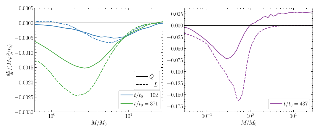
Figure 2: The mass-integrated, temperature-weighted time derivative of the specific entropy (solid) and the theoretical conductive luminosity (dashed) at three points in the evolution, corresponding to Fig. 1. The late evolution is shown on a separate panel due to the differing scales of interest.

The fluid model closes the Boltzmann hierarchy by adopting an ideal gas equation of state and Fourier’s law of thermal conductivity. This is analogous to the treatment of proto-stellar evolution, except in that case energy is transported by radiation or convection rather than conduction (e. g. [29, 30, 12]). A similar model has also been applied to the evolution of globular clusters due to two-body gravitational scattering events, e. g. [16].

Specifically, the second moment of the Boltzmann equation yields, for an ideal gas, the energy equation [3]:

$$-\left(\frac{\partial L}{\partial M}\right)_{t}=\frac{{\langle\mathbf{v}^{2}\rangle}}{3}\left(\frac{\mathrm{d}s_{\mathrm{I}}}{\mathrm{d}t}\right)_{M}$$ (2)

with $L$ the luminosity, $M$ the (enclosed) mass, and $s_{\mathrm{I}}=\ln(\langle\mathbf{v}\rangle^{3}/\rho)$ the specific entropy (up to an additive constant) of a monatomic ideal gas. The factor of three relates the 3D velocity dispersion $\langle\mathbf{v}^{2}\rangle$ to the temperature. This equation is also a statement of the first law of thermodynamics. In the presence of anisotropic (viscous) stress, this equation must be amended:

$$-\left(\frac{\partial L}{\partial M}\right)_{t}+\pi_{ij}\frac{\partial u_{i}}{\partial x_{j}}=\frac{{\langle\mathbf{v}^{2}\rangle}}{3}\left(\frac{\mathrm{d}s_{\mathrm{I}}}{\mathrm{d}t}\right)_{M},$$ (3)

where $\pi_{ij}=-\langle v_{i}v_{j}\rangle+\frac{1}{3}{\langle\mathbf{v}^{2}\rangle}\delta_{ij}$ and $\mathbf{u}=\langle\mathbf{v}\rangle$ is the bulk velocity.

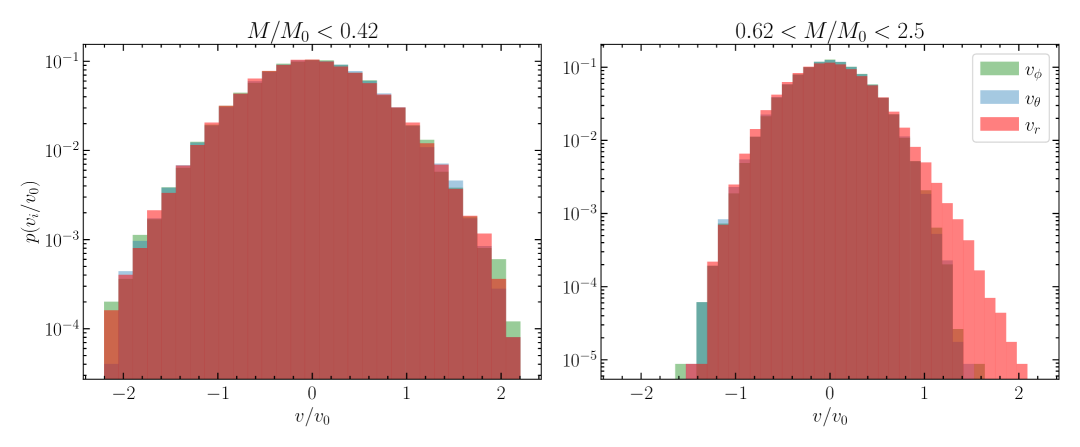
Figure 3: The velocity distribution function at a late time ($t/t_{0}=437$) in the SMFP core (left) and in the IMFP region (right).

Due to the anisotropy in the velocity distribution function (Fig. 1), we should expect energy transport by viscous dissipation in addition to conduction. We examine this hypothesis directly by comparing the conductive luminosity with the entropy production rate. In the conducting fluid model, the following form is adopted for the luminosity:

$$\frac{L}{4\pi r^{2}}=-\frac{1}{2}a\sqrt{\frac{{\langle\mathbf{v}^{2}\rangle}}{3}}\left(\frac{12\pi G}{C\rho{\langle\mathbf{v}^{2}\rangle}\sigma_{m}}+\frac{a}{b}\sigma_{m}\right)^{-1}\frac{\partial{\langle\mathbf{v}^{2}\rangle}}{\partial r},$$ (4)

with $a=4/\sqrt{\pi}$, $b=25\sqrt{\pi}/32$, and $C$ an unknown constant of order unity. The first term in parentheses is an approximate form of the LMFP thermal conductivity [16, 3], while the second term can be exactly derived in the SMFP limit [6]. Here, we adopt $C=0.84$ (as in [24], which is similar to the case studied here). We interrogate the fluid model quantitatively by comparing the luminosity with the integral of the right-hand side of Eq. 2,

$$\dot{Q}\equiv\int dM\,\frac{{\langle\mathbf{v}^{2}\rangle}}{3}\left(\frac{\mathrm{d}s_{\mathrm{I}}}{\mathrm{d}t}\right)_{M},$$ (5)

Accordingly, both sides of Eq. 2, integrated over mass, are shown in Fig. 2. In blue in the left panel, the entire halo is in the LMFP regime and the two expressions agree well. In green the core has entered the IMFP regime and shows worse agreement. In purple (right panel) the expressions agree in the SMFP core, but in the IMFP regime the agreement is again poor, and we have an asymptotic value of $\dot{Q}>0$, which indicates a breakdown of the conducting fluid model: equating this quantity with the luminosity would require heat flow against the temperature gradient. The deviation is naturally explained by viscous dissipation sourced in the IMFP regime.

In Fig. 3 we show directly the velocity distribution in the SMFP (left) and IMFP (right) regimes. In the IMFP regime the outward heat flux in the radial direction has not fully thermalized, and the distribution function is not isotropic. Indeed, LTE is a fundamental assumption entering the fluid model in both the energy transport (2) and luminosity (4) equations: Eq. 4 assumes a well-defined local temperature while Eq. 2 omits the viscous dissipation which is associated with anisotropy in the velocity distribution function.

Although LTE is established deep in the core, the structure of the core (i. e. the slope of the density and velocity dispersion profiles near the core boundary) remains sensitive to the IMFP behavior. This is because the luminosity peaks in the IMFP regime, such that the evolutionary (Kelvin–Helmholtz) timescale hardly varies as a function of mass enclosed between the core and the IMFP region. In other words, the IMFP region is evolving on a similar timescale to the core. Figure 4 shows these differences between the DSMC and fluid results at matched central densities. Although the central velocity dispersions are similar, the evolution outside of the core is qualitatively different between the two treatments. In the fluid model the core boundary becomes increasingly sharp over time as the velocity dispersion increases in the inner region and decreases in the outer region. Meanwhile, in the kinetic treatment the viscous heating leads to very slow evolution in the velocity dispersion outside the core.

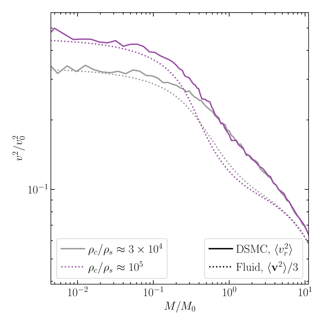
Figure 4: The DSMC radial velocity dispersion (solid) and fluid 1D velocity dispersions (dashed) when the central density $\rho_{\mathrm{c}}$ is $\rho_{\mathrm{c}}/\rho_{\mathrm{s}}\sim 4\times 10^{4}$ (silver) and $\rho_{\mathrm{c}}/\rho_{\mathrm{s}}\sim 4\times 10^{5}$ (purple).

IV Discussion

We have developed the new Direct Simulation Monte Carlo code KiSS-SIDM to study the gravothermal evolution of self-interacting dark matter halos. By exploiting the spherical symmetry in the idealized collapse problem and implementing a more efficient scattering algorithm, our code improves substantially on the speed and accuracy of previous $N$-body methods. This allows us to simulate the collapse well into the short mean free path regime using a fully kinetic method.

In the IMFP region, we find qualitative disagreement with the fluid model due to the non-equilibrium state of the DM. In the canonical case studied here most of the evolutionary time is spent in the LMFP regime. Thus, the deviations from LTE result in only a negligible effect on the core collapse timescale and corresponding observational constraints. However, recent work has identified differences of $\sim$30\text{\,}\mathrm{\char 37\relax}$$ in the collapse time and minimal core density between different $N$-body SIDM implementations. In this context, the DSMC method will be an independent test and comparison point. Further, the non-equilibrium effects uncovered in this minimal SIDM scenario serve as a cautionary note for the study of more complex dark sectors containing both an elastic scattering self-interaction and other physics, such as dissipation (e. g. [7]).

On the other hand, there is long-standing interest in the possibility that core collapse in SIDM halos could explain the presence of supermassive black holes in galactic centers [3, 27, 8, 13, 10]. There, the key parameter is the core mass at the time when relativistic instability induces dynamical collapse, which these studies have investigated by extrapolating fluid model results to very high central densities. Our results confirm that deep in the SMFP regime LTE is established and the conducting fluid model is appropriate. Nonetheless, the non-equilibrium IMFP region remains relevant deep into the collapse.

Ref. [3] argues that the mass enclosed within the IMFP region sets the mass of the final black hole, as interior to this scale the DM will respond hydrodynamically (i. e. collapse) due to a loss of pressure support in the core, while in the LMFP region a new (nearly) collisionless equilibrium will be established. In the fluid model, the density and velocity dispersion profiles in the IMFP region continue to evolve even when the core is deep into the SMFP evolution. The difference between the fluid model and our simulation result is still increasing at the end of our simulation, while the central density and velocity dispersion remain many orders of magnitude below the relativistic instability threshold. Thus, it is dangerous to study the core structure at late times using the fluid model.

In particular, the late-time evolution in the fluid treatment has been described in terms of simple power-law scalings [3, 10, 23]. It is not yet clear whether an analogous self-similarity arises in the kinetic treatment. Likewise, in the fluid model the evolution is “universal” in that $\sigma_{m}/\sigma_{0}$ is the only parameter controlling the dynamics in initially NFW halos, but it is possible that the viscous heating identified here introduces a parametrically different time dependence and hence a broader range of collapse behaviors.

In the future, it will be particularly interesting to apply the DSMC method to anisotropic, velocity-dependent cross sections. Because a large cross section is not observationally excluded at low velocities, the halo may enter the IMFP regime at earlier times and lower densities. Moreover, both the high-temperature cutoff in the cross section and a differential cross section favoring forward/backward scattering may substantially impede thermalization of the distribution function at high densities.

Acknowledgments.

We thank Neal Dalal, Moritz Fischer, Laura Sagunski, and Kimberly Boddy for useful discussions. We thank Michael Ryan for sharing a modified version of the SpherIC initial conditions generator. Research at the Perimeter Institute is supported in part by the Government of Canada through the Department of Innovation, Science and Economic Development Canada and by the Province of Ontario through the Ministry of Colleges and Universities.

End Matter

Appendix A Details of the Direct Simulation Monte Carlo Code KiSS-SIDM

Here, we provide a more detailed account of the numerical methods and implementation details of our code KiSS-SIDM. In our DSMC algorithm, space is discretized into a grid whose cells are smaller than the mean free path, and scattering between particles can only occur within a single cell. For the majorant collision frequency scheme, the following upper bound on the number of collisions in each cell is calculated at each time step $\Delta t$:

$$\Gamma_{i}=N_{i}\rho_{i}\sigma_{m,\mathrm{max},i}v_{\mathrm{max},i}\Delta t,$$ (6)

where $N_{i}$ is the number of tracers in the cell $i$, $\rho_{i}$ is the mass density in this cell, $\sigma_{m,\mathrm{max},i}$ is an upper bound on on the cross section (per unit mass), $v_{\mathrm{max},i}$ is an upper bound on the relative velocity between particles, and $\Delta t$ is the time step.

The collision time step is chosen as

$$\Delta t_{\mathrm{coll}}=\min_{i}\left(\frac{\lambda_{\mathrm{MFP},i}}{v_{\mathrm{max},i}}\right)$$ (7)

where

$$\lambda_{\mathrm{MFP},i}=\frac{1}{\rho_{i}\sigma_{m,\mathrm{max},i}}$$ (8)

is an estimate of the mean free path within cell $i$.

At each timestep, and in each cell $\Gamma_{i}$ pairs (trial pairs) are sampled. Each trial pair of particles collides if:

$$\frac{\sigma_{m}(v_{\mathrm{rel}})v_{\mathrm{rel}}}{\sigma_{m,\mathrm{max},i}v_{\mathrm{max},i}}>q,$$ (9)

where $\sigma_{m}$ is the cross section per unit mass and $q$ is randomly drawn from a uniform distribution on $[0,1)$. Multiple scatterings of the same particle pairs are not explicitly forbidden. This issue of repeated scattering becomes negligible when the number of particles per cell is large: [2] mention a rule of thumb that when this number exceeds 10 repeated scatterings do not require any special handling. This condition is satisfied in our simulations.

We assume spherical symmetry by recording only the radial position coordinate $r$ and the velocity components $\mathbf{v}=(v_{r},v_{\phi},v_{\theta})$. At each time step the 3D (Cartesian) coordinates of each particle are first updated as

$$\mathbf{x^{\prime}}=r\mathbf{\hat{r}}+\mathbf{v}\Delta t.$$ (10)

Then the new angular basis is formed from $\mathbf{\hat{r}^{\prime}}=\mathbf{x^{\prime}}/|\mathbf{x^{\prime}}|$ and a pair of orthonormal tangential vectors. The velocity components are rotated into this new $\mathbf{\hat{r}^{\prime}}$, $\mathbf{\hat{\phi}^{\prime}}$, $\mathbf{\hat{\theta}^{\prime}}$ basis and stored. Finally, the new radial coordinate is calculated as $r^{\prime}=|\mathbf{x^{\prime}}|$ and stored.

As mentioned above, all particles within one spherical shell (grid cell) can scatter. The gravitational force is similarly simplified by spherical symmetry. The gravitational acceleration on each particle is

$$a_{\mathrm{g}}=\frac{GM_{\mathrm{enc}}}{r^{2}},$$ (11)

where $M_{\mathrm{enc}}$ is the mass interior to the particle. Within each cell, we smooth the mass distribution (and reduce the computational cost) by approximating the cumulative mass function as locally log-linear: $M(r)=M_{i}(r/r_{i})^{\alpha}$, where $M_{i}$ is the mass enclosed at the lower boundary $r_{i}$ of the cell, and $\alpha$ is chosen to ensure continuity of the cumulative mass enclosed between cells. Note that the grid used for the collision and gravity steps does not necessarily need to be the same; however, we have chosen to identify the two for simplicity in our code. The gravitational time step is determined via

$$\Delta t_{\mathrm{grav}}=\epsilon\min_{i}\left(t_{\mathrm{ff},i}\right),$$ (12)

where we choose $$\epsilon=$0.02$$$ and

$$t_{\mathrm{ff},i}=\frac{1}{\sqrt{G\bar{\rho}_{i}}}$$ (13)

is the free-fall time in grid cell $i$, with the average density $\bar{\rho}_{i}$ within the sphere that reaches the center of the cell. The total time step is

$$\Delta t=\min(\Delta t_{\mathrm{coll}},\Delta t_{\mathrm{grav}}).$$ (14)

As the simulation proceeds, the mean free path within each cell, as well as the required spatial resolution for the gravitational accelerations, changes with the evolution. In order to ensure that the grid is fine enough at all times, we split grid cells into two once the mean free path (Eq. 8) becomes smaller than the grid cell. Similarly, we split cells if the fraction $f_{\mathrm{J}}$ of the Jeans length $\lambda_{\mathrm{J},i}$ within the cell,

$$\lambda_{\mathrm{J},i}=\sqrt{\frac{{\langle\mathbf{v}^{2}\rangle}_{i}}{G\rho_{i}}},$$ (15)

becomes smaller than the cell size (choosing $f_{\mathrm{J}}=1/20$). However, cells are only split if they contain a minimum number of particles, $n_{\rm min}=32$.

For the time integration, we divide each time step as

$$K(\Delta t/2)\,S(\Delta t/2)\,D(\Delta t)\,S(\Delta t/2)\,K(\Delta t/2),$$ (16)

where $K$ is the gravitational kick, $D$ the position update (“drift”), and $S$ the scattering. This formulation is not exactly time reversible due to the stochasticity of the scattering and the non-reversibility of the time step, yet it produces good long-term accuracy in our testing. The code makes use of shared-memory parallelization (threading).

Concerning the analysis, the curves in Figs. 1, 2 and 4 are averages over closely spaced snapshots to control the noise due to limited particle number. It can be noted that our use of the integrated quantities $L$ and $\dot{Q}$ avoids noisy numerical derivatives required to evaluate both sides of Eq. 2 directly in the simulation data. Still, Eq. 4 requires a spatial derivative of the velocity dispersion, which leads to artifacts in the core region, where the gradient is small. In Fig. 3, we have not subtracted the bulk velocity, in order to emphasize that the radial distribution function has a mode near zero and differs from the angular components in the tails.

References

- Adhikari et al. [2022] Adhikari, S., Banerjee, A., Boddy, K. K., et al. 2022, Astrophysical Tests of Dark Matter Self-Interactions. https://arxiv.org/abs/2207.10638
- Akhlaghi et al. [2018] Akhlaghi, H., Roohi, E., & Stefanov, S. 2018, Computers & Fluids, 161, 23, doi: https://doi.org/10.1016/j.compfluid.2017.11.005
- Balberg & Shapiro [2002] Balberg, S., & Shapiro, S. L. 2002, Phys. Rev. Lett., 88, doi: 10.1103/physrevlett.88.101301
- Bird [1994] Bird, G. 1994, Molecular Gas Dynamics and the Direct Simulation of Gas Flows, Vol. 1 (Clarendon Press)
- Burkert [2000] Burkert, A. 2000, ApJ, 534, L143, doi: 10.1086/312674
- Chapman & Cowling [1970] Chapman, S., & Cowling, T. G. 1970, The mathematical theory of non-uniform gases. an account of the kinetic theory of viscosity, thermal conduction and diffusion in gases (Cambridge University Press)
- Essig et al. [2019] Essig, R., McDermott, S. D., Yu, H.-B., & Zhong, Y.-M. 2019, Phys. Rev. Lett., 123, doi: 10.1103/physrevlett.123.121102
- Feng et al. [2021] Feng, W.-X., Yu, H.-B., & Zhong, Y.-M. 2021, ApJ, 914, L26, doi: 10.3847/2041-8213/ac04b0
- Fischer et al. [2024] Fischer, M. S., Dolag, K., & Yu, H.-B. 2024, A&A, 689, A300, doi: 10.1051/0004-6361/202449849
- Gad-Nasr et al. [2024] Gad-Nasr, S., Boddy, K. K., Kaplinghat, M., Outmezguine, N. J., & Sagunski, L. 2024, JCAP, 05, 131, doi: 10.1088/1475-7516/2024/05/131
- Garrison-Kimmel et al. [2013] Garrison-Kimmel, S., Rocha, M., Boylan-Kolchin, M., Bullock, J. S., & Lally, J. 2013, MNRAS, 433, 3539–3546, doi: 10.1093/mnras/stt984
- Hosokawa & Omukai [2009] Hosokawa, T., & Omukai, K. 2009, ApJ, 691, 823, doi: 10.1088/0004-637X/691/1/823
- Jiang et al. [2025] Jiang, F., Jia, Z., Zheng, H., et al. 2025, Formation of the Little Red Dots from the Core-collapse of Self-interacting Dark Matter Halos. https://arxiv.org/abs/2503.23710
- Kamada et al. [2017] Kamada, A., Kaplinghat, M., Pace, A. B., & Yu, H.-B. 2017, Phys. Rev. Lett., 119, 111102, doi: 10.1103/PhysRevLett.119.111102
- Koda & Shapiro [2011] Koda, J., & Shapiro, P. R. 2011, MNRAS, 415, 1125, doi: 10.1111/j.1365-2966.2011.18684.x
- Lynden-Bell & Eggleton [1980] Lynden-Bell, D., & Eggleton, P. P. 1980, MNRAS, 191, 483, doi: 10.1093/mnras/191.3.483
- Mace et al. [2025] Mace, C., Yang, S., Zeng, Z. C., et al. 2025, Calibrating the SIDM Gravothermal Catastrophe with N-body Simulations. https://arxiv.org/abs/2504.13004
- Mace et al. [2024] Mace, C., Zeng, Z. C., Peter, A. H. G., et al. 2024, Convergence Tests of Self-Interacting Dark Matter Simulations. https://arxiv.org/abs/2402.01604
- Meskhidze et al. [2022] Meskhidze, H., Mercado, F. J., Sameie, O., et al. 2022, MNRAS, 513, 2600–2608, doi: 10.1093/mnras/stac1056
- Navarro et al. [1997] Navarro, J. F., Frenk, C. S., & White, S. D. M. 1997, ApJ, 490, 493, doi: 10.1086/304888
- Nishikawa et al. [2020] Nishikawa, H., Boddy, K. K., & Kaplinghat, M. 2020, Phys. Rev. D, 101, doi: 10.1103/physrevd.101.063009
- Oran et al. [1998] Oran, E., Oh, C., & Cybyk, B. 1998, Annual Review of Fluid Mechanics, 30, 403, doi: 10.1146/annurev.fluid.30.1.403
- Outmezguine et al. [2023] Outmezguine, N. J., Boddy, K. K., Gad-Nasr, S., Kaplinghat, M., & Sagunski, L. 2023, MNRAS, 523, 4786, doi: 10.1093/mnras/stad1705
- Palubski et al. [2024] Palubski, I., Slone, O., Kaplinghat, M., Lisanti, M., & Jiang, F. 2024, J. Cosmology Astropart. Phys, 2024, 074, doi: 10.1088/1475-7516/2024/09/074
- Pareschi, Lorenzo & Russo, Giovanni [2001] Pareschi, Lorenzo, & Russo, Giovanni. 2001, ESAIM: Proc., 10, 35, doi: 10.1051/proc:2001004
- Peter et al. [2013] Peter, A. H. G., Rocha, M., Bullock, J. S., & Kaplinghat, M. 2013, MNRAS, 430, 105–120, doi: 10.1093/mnras/sts535
- Pollack et al. [2015] Pollack, J., Spergel, D. N., & Steinhardt, P. J. 2015, ApJ, 804, 131, doi: 10.1088/0004-637X/804/2/131
- Rocha et al. [2013] Rocha, M., Peter, A. H. G., Bullock, J. S., et al. 2013, MNRAS, 430, 81, doi: 10.1093/mnras/sts514
- Stahler et al. [1980a] Stahler, S. W., Shu, F. H., & Taam, R. E. 1980a, ApJ, 241, 637, doi: 10.1086/158377
- Stahler et al. [1980b] —. 1980b, ApJ, 242, 226, doi: 10.1086/158459
- Tulin & Yu [2018] Tulin, S., & Yu, H.-B. 2018, Physics Reports, 730, 1–57, doi: 10.1016/j.physrep.2017.11.004
- Turner et al. [2021] Turner, H. C., Lovell, M. R., Zavala, J., & Vogelsberger, M. 2021, MNRAS, 505, 5327–5339, doi: 10.1093/mnras/stab1725
- Yang et al. [2023] Yang, S., Du, X., Zeng, Z. C., et al. 2023, ApJ, 946, 47, doi: 10.3847/1538-4357/acbd49