The bearable inhomogeneity of the baryon asymmetry

Abstract

We study the implications of precision measurements of light element abundances in concordance with the Cosmic Microwave Background for scenarios of physics beyond the Standard Model that generate large inhomogeneities in the baryon-to-photon ratio. We show that precision Big Bang Nucleosynthesis (BBN) imposes strong constraints on any mechanism that produces large scale inhomogeneities at temperatures of the order or below a TeV. In particular, we find that inhomogeneities of the order of $20\%$ at comoving length scales larger than the comoving horizon at the temperature of $3~\mathrm{TeV}$ are in conflict with the measured light element abundances. This sensitivity to physics at such early times is because inhomogeneities in baryon number homogenize predominantly through diffusion, which is a slow process. BBN therefore acts as a novel probe of baryogenesis below the $\mathrm{TeV}$ scale, and readily rules out some of the proposed scenarios of baryogenesis in the literature. We discuss the implications for electroweak baryogenesis. In addition we show that precision BBN is a new probe of first-order phase transitions which produce a gravitational wave signal in the frequency range from pHz to mHz. This leads to constraints on the electroweak phase transition, as well as the first-order phase transitions that have been postulated to explain the pulsar timing array signal. We also discuss the future prospects of improvements in this probe.

1 Introduction

In the era of precision cosmology, it is of great importance to leverage the available cosmological data as a new probe of physics beyond the standard model (BSM). The success of the theory of Big Bang Nucleosynthesis (BBN) in predicting the abundance of light elements matching their observed value makes BBN one of the most powerful and precise probes of the early universe. By combining measurements of primordial light element abundances with our understanding of the physics of BBN and with the measured nuclear reaction rates as input, the baryon-to-photon ratio $\eta$ can be determined. Independently, a measurement of $\eta$ to sub-percent precision is obtained from the angular power spectrum of the cosmic microwave background (CMB) Planck:2015fie ; Planck:2018vyg . The most precise BBN-based determination, dominated by the deuterium-to-hydrogen ratio $D/H$, achieves a precision of approximately $2\%$ Yeh:2022heq , and is in agreement with the value extracted from CMB. This close agreement between the BBN and CMB determinations of $\eta$ stands as a major success of modern cosmology. Currently, the dominant uncertainties in the BBN prediction of the baryon-to-photon ratio stem from that of nuclear reaction rates, making recent experimental advancements, such as those from the LUNA collaboration Mossa:2020gjc , particularly important for improving the uncertainty in the BBN predictions.

The CMB is a powerful probe of inhomogeneities in the early universe, in particular probing baryon isocurvature perturbations at the level of $O(10^{-5})$ Planck:2018jri . In this work, we explore how BBN also probes baryon isocurvature perturbations, i.e., inhomogeneities in the baryon-to-photon ratio, for the effect of adiabatic modes on BBN, see e.g. Inomata:2016uip ; Jeong:2014gna . The sensitivities of CMB and BBN to spatial inhomogeneities in $\eta$ differ significantly, offering complementary insights into potential physics beyond the standard cosmological model. In particular, while the level of precision from BBN is much less than that of the CMB, it probes length scales much smaller than those probed by the CMB. As we will show, BBN can be sensitive to comoving length scales that were sub-horizon even at electroweak temperatures, while CMB is primarily sensitive at comoving length scales of the order of and larger than the Hubble length at the time of recombination (see Planck:2018jri and e.g. Buckley:2025zgh for a recent study).

The deuterium-to-hydrogen ratio $D/H$ as the most sensitive probe of BBN in determining $\eta$, is particularly interesting in the context of sensitivity to inhomogeneities. In this regard, it is crucial that the final deuterium abundance depends non-linearly on the local value of $\eta$. Due to this non-linear dependence, two different spatial distributions of $\eta$ with the same average value generally lead to different predictions for the $D/H$ ratio. That is, averaging deuterium and hydrogen abundances over regions with varying baryon densities does not erase the effects of small-scale fluctuations in $\eta$. Assuming small fluctuations around its mean value, one can expand the final abundances in terms of the relative size of the fluctuations. While the linear term averages out, higher order terms lead to different prediction from homogeneous BBN. To obtain a rough estimate, if we assume an $O(1)$ coefficient for the second-order terms in such an expansion, a percent-level measurement of $D/H$ can be sensitive to $\mathcal{O}(10\%)$ variations in $\eta$. This sensitivity is to fluctuations on all length scales that survive until BBN, in particular their length scale can be much smaller than horizon size at the time of BBN.

A remarkable observation that we emphasize in this work is that inhomogeneities introduced at times much earlier than the BBN could survive until then and therefore be probed. This applies not only to superhorizon fluctuations, but also to ones with length scale well within the horizon at the time of nucleosynthesis. To understand the reach of BBN as a probe of early times, we must therefore consider the evolution of sub-horizon inhomogeneities in $\eta$. For small fluctuations, the dominant mechanism for homogenizing baryons is diffusion. As the temperature $T$ drops in a radiation dominated universe, the mean free path of the particles (and the diffusion constants) tend to grow, and the time scale for diffusion, set by the inverse Hubble scale $H^{-1}$ becomes larger. Therefore the effect of the diffusion is dominated by the latest times. The available time for diffusion is $t\sim H^{-1}\sim M_{\text{Pl}}/T^{2}$, while the typical interaction time and length scale for a strongly coupled system are $\tau\sim l_{\text{mfp}}\sim 1/T$. A particle therefore undergoes $N\sim t/\tau$ scatterings, and its random-walk leads to a diffusion distance $d\sim\sqrt{N}l_{\text{mfp}}$. Comparing this to the Hubble length $l_{H}\sim H^{-1}$ gives $d/l_{H}\sim\sqrt{T/M_{\text{Pl}}}\ll 1$, indicating that diffusion is inefficient at erasing inhomogeneities unless they are on length scales orders of magnitude smaller than the horizon scale at late times.

It is instructive to estimate the earliest time at which sub-horizon inhomogeneities can be produced and still survive until BBN. Imagine perturbations are generated with horizon size at some temperature $T_{i}\,$. Due to cosmic expansion, the length scale of these inhomogeneities grows to $(a_{\text{BBN}}/a_{i})\cdot l_{H}(T_{i})\sim(T_{i}/T_{\text{BBN}})\cdot l_{H}(T_{i})$ by the time of BBN, where the $a$’s are the corresponding scale factors. Comparing this with the diffusion length at BBN, $d\sim\sqrt{M_{\text{Pl}}/T_{\text{BBN}}}\cdot l_{H}(T_{\text{BBN}})$, fluctuations survive if $T_{i}\lesssim\sqrt{T_{\text{BBN}}M_{\text{Pl}}}\sim 10^{4}$ TeV. This naive estimate assumes strong coupling of baryons to the plasma, but in reality, at the relevant temperatures neutrons are weakly coupled to the plasma and dominate the baryon diffusion. A more refined treatment (see section 2) yields $T_{i}\lesssim 3~\mathrm{TeV}\,$. Thus, horizon-scale inhomogeneities seeded at temperatures of a few $\mathrm{TeV}$ can just barely evade diffusion and survive to influence BBN, offering a tantalizing window into high-energy physics in the early universe.

We find that inhomogeneities greater than $\mathcal{O}(20-30\%)$ that are generated over distances larger than $\mathcal{O}(H^{-1})$ at temperatures of a few $\mathrm{TeV}$ are incompatible with the measured light element abundances. This novel constraint on the early universe has exciting consequences, some of which we briefly explore. It readily rules out a recently proposed mechanism of baryogenesis Elor:2024cea which produces baryons very inhomogeneously, can test electroweak baryogenesis (EWBG) using domain walls Azzola:2024pzq , and perhaps most importantly is a novel probe of standard electroweak baryogenesis. Furthermore, it tests all kind of models that imprint inhomogeneities at the relevant length scales on a pre-existing background of baryon (or equally well $B-L$) asymmetry, such as a strong first-order phase transition in the early universe.

The first studies of the evolution of inhomogeneities and their effect on BBN were already performed in the 80’s Applegate:1985qt ; Applegate:1987hm , with subsequent refinement of the treatment of diffusion 1990ApJ…358…36M ; Kurki-Suonio:1992knt ; Suh:1998nt . In Jedamzik:1993tcf ; Jedamzik:1993dc the authors follow baryon inhomogeneities from early times until BBN, considering not only baryon diffusion which is the dominant process for small inhomogeneities, but also the effect of heat conduction via neutrino (see also Heckler:1993nc where the latter effect was considered and found to be important only for very large baryon overdensities). In the absence of concordance between CMB and BBN at the time, and within BBN data itself, early works also studied if inhomogeneities during BBN can bring them into agreement Jedamzik:2001qc ; Kainulainen:1998vh . The possibility of constraining electroweak baryogenesis was already discussed in Fuller:1993sp ; Heckler:1994uu ; Megevand:2004ry ; Brandenberger:1994fe . Note that at the time of these earlier studies, due to lack of precision CMB data, $\eta$ was still a free parameter for BBN. Its value was only determined later through precision measurements of the CMB, most notably by the Wilkinson Microwave Anisotropy Probe (WMAP) WMAP:2003ivt , and subsequently refined by the Planck satellite Planck:2018vyg .

More recently, the effect of inhomogeneities on BBN was reconsidered in Barrow:2018yyg ; Inomata:2018htm . The analysis of these works was limited to length scales larger than the neutron diffusion length scale at BBN, such that diffusion until BBN can be neglected. In our analysis, we additionally consider length scales that are smaller than the neutron diffusion lengths at BBN. This is particularly important, since these small length scales are the ones that probe the universe at its earliest time. Our results differ from those of Barrow:2018yyg ; Inomata:2018htm , even for the length scale where neutron diffusion can be ignored. The difference arises because in order to find the $D/H$ ratio, we separately average over deuterium and hydrogen densities. Additionally, in our study of baryon diffusion we improve on previous studies, by solving the coupled Boltzmann equations for neutrons and protons including diffusion. This is particularly important in determining the evolution of proton inhomogeneities.

This work is organized as follows: In section 2 we explain the big picture and follow the inhomogeneities in baryon-to-photon ratio from early times until BBN by solving the coupled diffusion equations of protons and neutrons. In section 3, we first review BBN and then derive the allowed magnitude of the inhomogeneities during BBN. For this purpose, we use the PRyMordial package Burns:2023sgx to obtain the dependence of the light element abundances on local proton and neutron densities. Finally in section 4 we study various scenarios that produce inhomogeneities in the baryon-to-photon ratio and are constrained by our work. This includes models of baryogenesis and scenarios which source a large gravitational wave signal.

2 Homogenization of baryons by diffusion

In this section, we study the evolution of inhomogeneities in the baryon asymmetry, starting from early times until and during the BBN. Considering small-amplitude inhomogeneities, this is governed by baryon diffusion.

2.1 Estimates and big picture

In this subsection, we give a first estimate of the diffusion length of baryons and the evolution of inhomogeneities in baryon number. A more rigorous treatment will be presented in the next subsection.

We write the FRW metric as

$$ds^{2}=dt^{2}-a^{2}d\vec{x}^{2}\,,$$ (1)

where $a$ is the scale factor and $\vec{x}$ denotes the comoving spatial coordinates. The diffusion equation for a comoving charge density $n$ is given by

$$\frac{\partial n}{\partial t}=D\nabla^{2}n\,,$$ (2)

where $D$ is the diffusion coefficient. Here, $\nabla^{2}=\nabla_{i}\nabla^{i}=\sum_{i}a^{-2}\partial_{i}\partial_{i}$. For simplicity, in this subsection we use the relation $a(t)\propto T^{-1}$, neglecting modifications that arise when different species (e.g., electrons) become nonrelativistic. Then we can write the Hubble scale as

$$H\equiv\frac{\dot{a}}{a}=-\frac{1}{T}\frac{\partial T}{\partial t}\,,$$ (3)

which we can use to rewrite eq. (2) as,

$$-HT\frac{\partial n}{\partial T}=D\,\frac{T^{2}}{T_{0}^{2}}\,\partial_{x}^{2}n\,,$$ (4)

where $T_{0}$ denotes a reference temperature at which we normalize $a(T_{0})=1$. The Hubble parameter during radiation domination is given by

$$H=\frac{\pi}{3}\frac{T^{2}}{M_{\text{Pl}}}\left(\frac{g_{*}(T)}{10}\right)^{1/2}\,,$$ (5)

where $g_{*}(T)$ is the effective number of relativistic degrees of freedom and $M_{\text{Pl}}\simeq 2.4\cdot 10^{18}\,\text{GeV}$ is the reduced Planck mass. For now, we approximate $g_{*}(T)\simeq 10.75$, while we will incorporate its full $T$ dependence in the next subsection.

We are interested in determining the evolution of inhomogeneities in the baryon number density. To this end, we solve the corresponding diffusion equations. Before neutrino decoupling, the rates converting protons to neutrons and vice versa are faster than the Hubble rate, so we can treat their diffusion together. Let us first consider temperatures $T\gtrsim 1\,\rm{MeV}$. Suppose there is some initial distribution of the baryon number density at a temperature $T_{i}$, well above the $\mathrm{MeV}$ scale. The effect of diffusion on this distribution is generally dominated by the lowest temperatures in the range considered, since as $T$ drops: (1) the Hubble scale drops, allowing more time for diffusion; and (2) interaction rates decrease, leading to larger diffusion coefficients.

At temperatures $T\sim\mathrm{MeV}$, baryon diffusion is dominated by scattering with electrons. The mean free path of neutrons is much larger than that of protons because the proton is charged, while the neutron is electrically neutral and interacts via its magnetic dipole moment. Therefore, nucleons diffuse significantly only during the time they spend as neutrons. After neutrino decoupling, we must track the distributions of neutrons and protons separately: neutrons continue to diffuse, but proton-electron interactions are strong enough that proton diffusion between neutrino decoupling and BBN is negligible.

The diffusion equation can be solved in momentum space as

$$\tilde{n}_{k}(T)=\tilde{n}_{k}(T_{i})\exp\left[-k^{2}\int_{T}^{T_{i}}\mathrm{d}T\,\frac{T}{HT_{0}^{2}}D\right]\equiv\tilde{n}_{k}(T_{i})\exp\left[-\frac{d^{2}k^{2}}{2}\right]\,,$$ (6)

where $\tilde{n}_{k}$ denotes the Fourier transform of $n$ evaluated at comoving momentum $k$. Let us now estimate the neutron diffusion coefficient. The scattering of electrons (and positrons) via the neutron’s magnetic dipole moment has a cross section of the parametric form

$$\sigma_{ne}\sim\frac{\alpha^{2}\kappa^{2}}{m_{n}^{2}}\,,$$ (7)

where $\kappa=-1.29$ is the anomalous magnetic moment of the neutron in units of the nuclear magneton, and $m_{n}$ is the neutron mass. The diffusion coefficient can be estimated as $D\sim v_{n}^{2}\Delta t$, where $v_{n}$ is the neutron velocity and $\Delta t$ is the effective mean free time, i.e., the timescale over which a neutron changes direction. This leads to the estimate $D_{n}\sim(\sigma_{ne}\,\mathfrak{n}_{e})^{-1}$ for relativistic electrons ($T>m_{e}$), and $D_{n}\sim\sqrt{T/m_{e}}(\sigma_{ne}\,\mathfrak{n}_{e})^{-1}$ for non-relativistic electrons ($T<m_{e}$), where $\mathfrak{n}_{e}$ is the electron number density. Throughout the text, we use the symbol $\mathfrak{n}$ to denote number densities per proper volume, while we reserve $n$ for comoving number densities. Parametrically, we have

$$D_{n}\sim\frac{m_{n}^{2}}{\alpha^{2}\kappa^{2}T^{3}}\times\begin{cases}1&T>m_{e}\\ (T/m_{e})^{2}e^{m_{e}/T}&T<m_{e}\end{cases}\,.$$ (8)

We will obtain a more precise expression in the next subsection. This gives us an estimate for the proton diffusion length:

$$d_{p}=\left(-2\int_{T_{\text{dec}}}^{T_{i}}\mathrm{d}T\,X_{n}\frac{T}{HT_{0}^{2}}D_{n}\right)^{1/2}\simeq 10^{5}\,\text{cm}\,,$$ (9)

where we have chosen $T_{0}=1\,\rm{MeV}$, $T_{\text{dec}}\simeq 0.7\,\mathrm{MeV}$ is the neutrino decoupling temperature, and $X_{n}(T)$ is the fraction of time that nucleons spend as neutrons, and in equilibrium is given by $X_{n}^{\text{eq}}(T)=1/(1+e^{Q/T})$, with $Q=1.29\,\rm{MeV}$ denoting the neutron-proton mass difference. Evaluating $X_{n}$ at $T\sim T_{\rm dec}$, gives $X_{n}\simeq 1/6$. After $T_{\rm dec}$, and until the start of BBN, proton diffusion is negligible, but neutrons continue to diffuse. Therefore the neutron diffusion length—dominated by late times around when BBN takes place—can be estimated as

$$d_{n}=\left(-2\int_{T_{\text{BBN}}}^{T_{\text{dec}}}\mathrm{d}T\,\frac{T}{HT_{0}^{2}}D_{n}\right)^{1/2}\simeq 10^{7}\,\text{cm}\,,$$ (10)

with $T_{\text{BBN}}\simeq 0.06\,\mathrm{MeV}$.

To build an intuition for these length scales, let us compare them with the comoving Hubble scale at $100\,\text{GeV}$:

$$(aH)^{-1}\simeq 3\cdot 10^{5}\,\text{cm}\,,$$ (11)

where, again, we remind the reader that we have set the scale factor $a=1$ at $T_{0}=1\,\rm{MeV}$. We see that even if inhomogeneities are produced around electroweak temperatures at horizon scale, their length scale is large enough that proton inhomogeneities do not diffuse away before BBN. This means that BBN can probe inhomogeneities produced as early as the electroweak phase transition!

While we have now provided an intuitive picture and simple estimates of how far protons and neutrons diffuse before BBN, in the next subsection we refine these estimates by solving the coupled system of neutrons and protons across the temperature range of neutrino decoupling. In doing so, we keep the correct relationship between the scale factor $a$ and temperature $T$ across electron annihilation, and, of course, include all $\mathcal{O}(1)$ factors in the diffusion coefficients.

2.2 Diffusion equations and coefficients

In this subsection, we rigorously calculate the diffusion length scales for protons and neutrons. The Boltzmann equations for the comoving neutron and proton number densities are

$$\partial_{t}n_{n} =D_{n}\nabla^{2}n_{n}-\Gamma_{n\to p}n_{n}+\Gamma_{p\to n}n_{p}\,,$$ (12)

$$\partial_{t}n_{p} =D_{p}\nabla^{2}n_{p}+\Gamma_{n\to p}n_{n}-\Gamma_{p\to n}n_{p}\,,$$ (13)

where the rates consist of several processes,

$$\Gamma_{n\to p} =\gamma_{ne^{+}\to p\bar{\nu}}+\gamma_{n\nu\to pe}+\gamma_{n\to pe\bar{\nu}}\,,$$ (14)

$$\Gamma_{p\to n} =\gamma_{p\bar{\nu}\to ne^{+}}+\gamma_{pe\to n\nu}+\gamma_{pe\bar{\nu}\to n}\,,$$ (15)

with $\gamma_{x\to y}$ describing the thermal averaged rate of the process $x\to y$. Detailed balance relates the rates as

$$\gamma_{n\nu\to pe} =\gamma_{pe\to n\nu}\exp\left(-Q/T\right)\,,$$ (16)

$$\gamma_{ne^{+}\to p\bar{\nu}} =\gamma_{p\bar{\nu}\to ne^{+}}\exp\left(-Q/T\right)\,,$$ (17)

where $\gamma_{n\to pe\bar{\nu}}$ describes neutron decay with lifetime $\tau_{n}\simeq 878~\text{s}$, and the three-body rate $\gamma_{pe\bar{\nu}\to n}$ is negligible. The rates $\gamma_{n\nu\to pe}$ and $\gamma_{ne^{+}\to p\bar{\nu}}$ can be found, e.g., in Mukhanov:2003xs .

Using entropy conservation,

$$S\propto g_{*S}(T)T^{3}a^{3}=\text{const}\,,$$ (18)

we find

$$a(T)=\frac{T_{0}}{T}\left(\frac{g_{*S}(T_{0})}{g_{*S}(T)}\right)^{1/3}\,,$$ (19)

giving

$$\frac{\partial}{\partial t}=HT\left(1+\frac{1}{3}\frac{T}{g_{*S}(T)}\frac{\partial g_{*S}(T)}{\partial T}\right)^{-1}\frac{\partial}{\partial T}\,.$$ (20)

Substituting into the Boltzmann equations, we obtain in momentum space

$$\frac{HT}{1-\frac{1}{3}\frac{T}{g_{*S}(T)}\frac{\partial g_{*S}(T)}{\partial T}}\frac{\partial\tilde{n}_{k}^{(n)}}{\partial T}=\left(D_{n}k^{2}\left(\frac{T}{T_{0}}\right)^{2}\left(\frac{g_{*S}(T)}{g_{*S}(T_{0})}\right)^{2/3}-\Gamma_{n\to p}\right)\tilde{n}_{k}^{(n)}+\Gamma_{p\to n}\tilde{n}_{k}^{(p)}\,,$$ (21)

and

$$\frac{HT}{1-\frac{1}{3}\frac{T}{g_{*S}(T)}\frac{\partial g_{*S}(T)}{\partial T}}\frac{\partial\tilde{n}_{k}^{(p)}}{\partial T}=\left(D_{p}k^{2}\left(\frac{T}{T_{0}}\right)^{2}\left(\frac{g_{*S}(T)}{g_{*S}(T_{0})}\right)^{2/3}-\Gamma_{p\to n}\right)\tilde{n}_{k}^{(p)}+\Gamma_{n\to p}\tilde{n}_{k}^{(n)}\,,$$ (22)

where again we have normalized $a=1$ at a reference temperature $T_{0}$. Since the equations are linear in the number densities, the initial and final distributions are related simply by a transfer function (i.e. the retarded Green’s functions of the above equations). Once we have the temperature dependence of the diffusion coefficients $D_{n}$ and $D_{p}$ the coupled Boltzmann equations can be numerically integrated to determine the characteristic diffusion length as well as the full transfer functions. To be more explicit, given an initial distribution of the baryon asymmetry at an initial $T_{i}$ sufficiently above the MeV scale, we will have at later times

$$\tilde{n}_{k}^{(N)}(T)=\tilde{G}^{(N)}(k,T,T_{i})\,\tilde{n}_{k}^{(B)}(T_{i})\,,$$ (23)

where $\tilde{G}^{(N)}$ are the (momentum-space) Green’s functions describing the evolution of the density distributions with $N$ being either the neutron or the proton and $\tilde{n}_{k}^{(B)}$ denotes the Fourier transform of the comoving baryon number density, $n_{B}$. Note that we have used the fact that, for $T_{i}\gg\mathrm{MeV}$, the initial partition of $n_{B}$ into $n_{p}$ and $n_{n}$ has negligible effect on the final densities, as their ratios are rapidly driven toward equilibrium. Also for such $T_{i}$, $\tilde{G}^{(N)}$ are insensitive to $T_{i}$ and so we will drop it from the argument of $\tilde{G}^{(N)}$ in the rest of the paper. We denote $X_{N}(T)=\tilde{G}^{(N)}(k=0,T)$, so that as in the above, $X_{N}(T)$ denotes the ratio of spatially averaged densities of nucleons to that of baryons.

Neutron diffusion coefficient

For the temperatures relevant to our analysis, the leading process controlling neutron diffusion is scattering with electrons, with scattering off protons being subdominant. These combine according to

$$D_{n}^{-1}=D_{ne}^{-1}+D_{np}^{-1}\,.$$ (24)

The transport cross section for electron-neutron scattering is given by Applegate:1987hm

$$\sigma^{t}_{ne}=3\pi\frac{\alpha^{2}\kappa^{2}}{m_{n}^{2}}\,,$$ (25)

where $\kappa=-1.29$ is the anomalous magnetic moment of the neutron. Using this cross section, the corresponding diffusion coefficient can be obtained by first determining the mobility $b$, which relates the drag force $F$ to the particle velocity $V$ via $F=b^{-1}V$, and then using the Einstein relation $D=bT$ to relate the diffusion coefficient to the mobility. Assuming a Maxwell-Boltzmann distribution for the electrons, the diffusion coefficient is given by Applegate:1987hm

$$D_{ne}=\frac{\pi}{16}\left(\frac{m_{n}}{m_{e}}\right)^{2}\frac{1}{m_{e}(\alpha\kappa)^{2}}\frac{e^{1/x}}{x(1+3x+3x^{2})}\approx 0.67\frac{e^{1/x}}{x(1+3x+3x^{2})}~\text{cm}\,,$$ (26)

where $x\equiv T/m_{e}$. While the Maxwell–Boltzmann approximation is not strictly valid at high temperatures, its use introduces an error of less than $3\%$ even in that regime Applegate:1987hm . This expression exhibits the expected parametric behavior in both temperature regimes discussed in eq. (8) of the previous subsection.

We now discuss the contribution to the diffusion coefficient from neutron–proton scattering. The transport cross section for neutron-proton scattering is

$$\sigma_{np}=\frac{\pi a_{s}^{2}}{a_{s}^{2}k^{2}+(1-\frac{1}{2}r_{s}a_{s}k^{2})^{2}}+\frac{3\pi a_{t}^{2}}{a_{s}^{2}k^{2}+(1-\frac{1}{2}r_{t}a_{t}k^{2})^{2}}\,,$$ (27)

where $k$ is the nucleon momentum in the center‐of‐mass frame, and $a_{s}=-23.71~\mathrm{fm}$, $r_{s}=2.73~\mathrm{fm}$, $a_{t}=5.432~\mathrm{fm}$, $r_{t}=1.749~\mathrm{fm}$ are the isospin-singlet (s) and isospin-triplet (t) scattering lengths $a_{i}$ and effective ranges $r_{i}$. We use the corresponding diffusion coefficient obtained by ref. Jedamzik:2001qc given by

$$D_{np}=9.4\times 10^{-12}\left(\frac{T}{\mathrm{MeV}}\right)^{1/2}\frac{\mathrm{MeV}^{3}}{\mathfrak{n}_{p}}\times\frac{1}{I(a_{1},b_{1})+0.16I(a_{2},b_{2})}~\mathrm{cm}\,,$$ (28)

where

$$I(a,b)=\frac{1}{2}\int_{0}^{\infty}dx\frac{x^{2}e^{-x}}{ax+(1-bx/2)^{2}}\,,$$ (29)

and $a_{1}=13.59(T/\mathrm{MeV})$, $b_{1}=-1.56(T/\mathrm{MeV})$, $a_{2}=0.71(T/\mathrm{MeV})$, $b_{2}=0.23(T/\mathrm{MeV})$. In the low temperature limit eq. (28) simplifies to

$$D_{np}=\frac{3\sqrt{\pi}}{8}\frac{1}{\mathfrak{n}_{p}(\pi a_{s}^{2}+3\pi a_{t}^{2})}\left(\frac{T}{m_{N}}\right)^{1/2}\,.$$ (30)

Proton diffusion coefficient

As described above, protons remain in thermal equilibrium with neutrons until the time of neutrino decoupling, and their spatial homogenization is primarily governed by neutron diffusion during this period. The diffusion coefficient for protons is dominated by scattering with electrons. Following Applegate:1987hm , the proton diffusion coefficient is given by

$$D_{p}=\frac{3\pi}{8\alpha^{2}\Lambda(T)}\left(\frac{\hbar}{m_{e}}\right)\frac{xe^{1/x}}{1+2x+2x^{2}}\approx\frac{8.5\times 10^{-7}}{\Lambda(T)}\frac{xe^{1/x}}{1+2x+2x^{2}}~\text{cm}\,.$$ (31)

The divergence of cross section of Coulomb scattering in the forward region is cut off as the charge/potential is screened at distances larger than the Debye screening length. This is captured in the above equation by the Coulomb logarithm $\Lambda=\ln(2/\theta_{0})$, where $\theta_{0}^{2}=k_{d}^{2}/k_{\rm th}^{2}$ represents the square of the effective minimum scattering angle. Here, $k_{d}^{2}=4\pi\alpha\mathfrak{n}_{e}/T$ is the square of the Debye screening wave-vector, where $n_{e}$ is the sum of electron and positron number densities. The thermal wave-vector is given by $k_{\rm th}^{2}\sim 3m_{e}T$ in the non-relativistic regime and $k_{\rm th}^{2}\sim(3T)^{2}$ in the relativistic regime. The Coulomb logarithm is approximately constant, $\Lambda\approx 3.5$, at temperatures well above the electron mass ($T\gg m_{e}$), and increases to $\Lambda=\mathcal{O}(10)$ near BBN temperatures Applegate:1987hm .

Results of diffusion

We solve the coupled equations (21) and (22), using initial conditions in which protons and neutrons share the same momentum dependence and equilibrium number densities. At high temperatures, weak interaction rates are sufficiently rapid that any deviation from these initial conditions is quickly erased, and the system rapidly returns to equilibrium.

Analogous to the case where the transfer function is a simple Gaussian, we define the diffusion length $d_{i}=1/k_{0}^{i}$ via the momentum scale at which

$$\frac{\tilde{G}^{(i)}(k_{0}^{i},T)}{X_{i}(T)}=\exp[-1/2]\,,$$ (32)

for $i=n,p$. The temperature evolution of these diffusion lengths is shown in figure 1. These results can be compared with the naive estimates in eqs. (9) and (10). While the refined treatment alters the diffusion lengths by $\mathcal{O}(1)$ factors, the overall conclusion remains unchanged: If inhomogeneities are generated on comoving length scales larger than $\sim 1/30\,(aH)^{-1}(T=100~\text{GeV})$, they survive until BBN and may therefore be probed by the concordance between BBN and the CMB. To gain intuition about the significance of the diffusion length, in appendix B we present a toy model for the initial baryon inhomogeneities and follow its evolution due to diffusion. The transfer function for the neutron,$\tilde{G}^{(n)}$ , is well approximated by a Gaussian function as before since neutron diffusion is dominated by late times long after neutrino decoupling. However, the transfer function for protons $\tilde{G}^{(p)}$ being sensitive to the time of decoupling, deviates significantly from a Gaussian. In figure 2, we show the transfer function for the proton at $T=0.06~\mathrm{MeV}\simeq T_{\text{BBN}}$ and it is compared with a Gaussian transfer function with the same diffusion length.

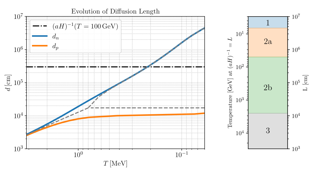
Figure 1: Evolution of the comoving diffusion length for protons and neutrons. The blue and yellow lines are obtained by solving the coupled eqs. (21) and (22). The dashed gray lines represent the naive estimates from eqs. (9) and (10). For comparison, the Hubble horizon size at $100~\mathrm{GeV}$ is shown as the horizontal dot-dashed black line. On the right panel we show the different regimes relevant for BBN depending on the characteristic comoving length scale $L$ of the inhomogeneities. For the description of each regime, see the discussion at the end of section 2.2. Note that we have set the scale factor to unity at $T=1\,\rm{MeV}$.

Depending on the length scale of the inhomogeneities, we need to consider different regimes. Let us assume that the inhomogeneities can be characterized by a comoving length scale $L$. Depending on the size of $L$ we can be in one of the following regimes: (1) For inhomogeneities on length scales larger than the neutron diffusion length, $L\gg d_{n}$, both neutron and proton inhomogeneities stay correlated and one can study the effect of inhomogeneities simply by varying $\eta$ and tracking the light element abundances as a function of its local value. (2) For inhomogeneities on length scales smaller than the neutron diffusion length and larger than the proton diffusion length, $d_{p}\ll L\ll d_{n}$, the inhomogeneities in protons are not altered, but neutrons are homogenized before BBN. In this regime there are also two distinct cases: (2.a) If neutron diffusion is slow compared to the rate at which neutrons are consumed to form deuterium, the neutron diffusion during BBN itself can be ignored, i.e.,

$$D_{n}(La)^{-2}\ll\langle\sigma_{np\rightarrow D\gamma}\,v\rangle n_{p}a^{-3}\,,$$ (33)

where $\sigma_{np\rightarrow D\gamma}$ is the cross section for deuterium production, $v$ the relative velocity and $\langle\ldots\rangle$ denotes the thermal average. This is the case for inhomogeneities with length scales larger than $\sim 6\,\rm{km}$ at the $\rm{MeV}$ temperature. In this case, the effect of inhomogeneities can be studied by considering the dependence of the abundances on the local proton density and a constant average neutron density. (2.b) For inhomogeneities that are on smaller length scales, but still larger than $d_{p}$, neutron diffusion during BBN is also important. In the more proton-rich regions, more neutrons are consumed as deuterium is formed, leading to a larger reduction of the neutron density, which subsequently draws more neutrons from the neighboring regions to keep the neutron density homogeneous. (3) Finally, if the length scale of inhomogeneities is smaller than the proton diffusion length, they are washed out before BBN. For example, from the transfer function of figure 2 we see that for length scale around $5d_{p}$, the amplitude of inhomogeneities are reduced by an order of magnitude. These different regimes are indicated in the right panel of figure 1.

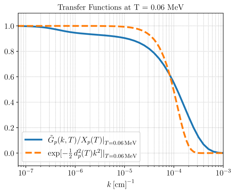
Figure 2: The transfer function for the proton number density obtained by solving the coupled diffusion equations. For comparison a Gaussian profile, which would be obtained from a simple decoupled diffusion equation, is shown by fixing its width such that is has the same $d_{p}$.

3 The tolerable inhomogeneity at BBN

In this section, we first review analytic estimates for the abundances of light elements, in particular ${}^{4}\mathrm{He}$ and $D$, and demonstrate why the $D/H$ ratio is especially sensitive to the value of $\eta$. This also gives an initial indication that the $D/H$ abundance depends non-linearly on both the baryon-to-photon ratio and the proton-to-neutron ratio. We then numerically evaluate the impact of inhomogeneities on the $D/H$ ratio using the PRyMordial package Burns:2023sgx . Our analysis leads to bounds on the allowed amplitude of inhomogeneities in the two regimes described in the previous section: (1) where both neutrons and protons stay inhomogeneous and (2) where neutrons homogenize but protons do not. We discuss the regimes (1), (2.a), and (2.b) in three different subsections, but leave a more detailed treatment of the case (2.b) to the appendix. We conclude the section by commenting on possible future improvements to these bounds.

3.1 A quick review of BBN

We briefly review the production of ${}^{4}\mathrm{He}$ and $D$. ${}^{4}\mathrm{He}$ is the most tightly bound of the light nuclei, and nearly all surviving neutrons are incorporated into it. This is because the rates that form heavier nuclei are small at the time when ${}^{4}\mathrm{He}$ is synthesized. As a result, estimating the ${}^{4}\mathrm{He}$ abundance mainly reduces to estimating the neutron abundance at the onset of BBN.

BBN begins when significant amount of deuterium has formed. In equilibrium, the deuterium-to-proton ratio is governed by the binding energy $B_{D}\simeq 2.2~\mathrm{MeV}$ and the baryon-to-photon ratio,

$$\left(\frac{n_{D}}{n_{p}}\right)_{\text{equil.}}\sim\mathfrak{n}_{n}\left(\frac{1}{m_{p}T}\right)^{3/2}e^{B_{D}/T}\propto\eta\left(\frac{T}{m_{p}}\right)^{3/2}e^{B_{D}/T}\,.$$ (34)

Due to the small value of $\eta$, significant deuterium production occurs only at temperatures well below the binding energy. The suppression is overcome at $T_{\text{BBN}}\simeq 60~\text{keV}$.

To estimate the neutron fraction at this temperature, note that while weak interactions remain in equilibrium,

$$\frac{n_{n}}{n_{p}}\simeq e^{-Q/T}\,,$$ (35)

where $Q\simeq 1.3~\mathrm{MeV}$ is the neutron–proton mass difference. These interactions freeze out around $T_{\nu}\simeq 0.8~\mathrm{MeV}$, giving $X_{n}(T_{\nu})\simeq 1/6$. From that point forward, only neutron decay alters the neutron abundance until BBN begins. Given the neutron lifetime $\tau_{n}\approx 878~\text{s}$, this leads to

$$X_{n}(T_{\text{BBN}})\simeq 1/8\,.$$ (36)

This simple estimate gives the mass fraction of ${}^{4}\mathrm{He}$ as

$$Y_{P}\equiv\frac{\rho(^{4}\text{He})}{\rho_{b}}\simeq 2X_{n}\simeq 0.25\,,$$ (37)

where $\rho({}^{4}\mathrm{He})$ and $\rho_{b}$ are the mass densities of ${}^{4}\mathrm{He}$ and baryons, respectively. The onset temperature of BBN depends only logarithmically on $\eta$, resulting in a weak dependence of $Y_{P}$ on $\eta$. Although $Y_{P}$ is measured to approximately $2\%$ precision, it constrains $\eta$ only at $\mathcal{O}(1)$. In principle, $Y_{P}$ is also sensitive to inhomogeneities in $\eta$, but only at a similar precision. As we now show, the $D/H$ ratio is a much more sensitive probe.

The final abundance of deuterium is set by its freeze-out. At that point, neutrons are no longer available to form new deuterium and the abundance decreases through three main reactions: $D+D\to{}^{3}\mathrm{He}+n$, $D+D\to{}^{3}\mathrm{H}+p$, and $D+p\to{}^{3}\mathrm{He}+\gamma$. The last of these, although suppressed by the electromagnetic coupling $\alpha$, becomes competitive at low enough $D$ abundances. This is critical. If the third reaction were negligible, the freeze-out deuterium abundance would be determined solely by the rates of the first two reactions and the Hubble expansion rate and would be insensitive to the local proton density. In such a case, the final deuterium to hydrogen ratio would depend on $\eta$ only through the average proton density and scales as $\langle D\rangle/\langle H\rangle\sim 1/\langle\eta\rangle$. Therefore in such a case, the deuterium-to-hydrogen ratio, $D/H$, would be insensitive to inhomogeneities.

On the other hand, if the third reaction dominates, the deuterium abundance becomes exponentially sensitive to the local proton density, and therefore to $\eta$. This would make $D/H$ highly sensitive to inhomogeneities in $\eta$. As shown in Mukhanov:2003xs , for $\eta\ll 10^{-9}$, the $D+D$ reactions dominate, while for $\eta\gg 10^{-9}$, the $D+p$ reaction dominates. At the observed value $\eta\simeq 6\cdot 10^{-10}$, both reactions compete, resulting in significant nonlinear dependence—and thus sensitivity to inhomogeneities in $\eta$. Because the competing rate depends on the proton density, the deuterium abundance becomes sensitive to spatial variations in the proton-to-neutron ratio. In the next subsection, we verify this expectation through a numerical study.

In this work, we adopt the viewpoint that the lithium problem arises from our incomplete understanding of astrophysical systems. An interesting question, however, is whether inhomogeneities during BBN could resolve this lithium discrepancy. For small fluctuations, it is easy to see that this is not the case: small fluctuations in $\eta$ after averaging always lead to a larger lithium abundance. For large amplitude fluctuations, the situation is more complicated. A naively promising scenario is the case when inhomogeneities are so large in amplitude that in some regions there are excess neutrons staying after helium formation. These neutrons can then diffuse to other regions, leading to a late time neutron injection. Scenarios of late time neutron injection have been discussed in the literature as a solution to the lithium problem AlbornozVasquez:2012emy ; Coc:2013eha , however more recent studies show that solving the lithium problem always introduces strong tension with the measured deuterium abundance Coc:2014gia .

3.2 Current constraints

In this section, we study the constraints on baryon inhomogeneities from BBN, considering three limiting cases. First, we examine the case where inhomogeneities are generated on large scales, such that neutron diffusion is too slow to homogenize the distribution before BBN. In this regime, the problem can be analyzed purely in terms of spatial variations in the baryon-to-photon ratio, $\eta$. Next, we consider the scenario where neutrons have completely homogenized before BBN, but protons have not. Depending on the length scale of the inhomogeneities, two distinct regimes emerge: one in which neutron diffusion during BBN can be neglected, and another in which it plays a significant role. We show in appendix A.1 that the final deuterium abundance in the latter case (2.b) is the same as in case (1), where inhomogeneities in protons and neutrons are correlated.

3.2.1 Inhomogeneity in $\eta$

We begin with the case where the inhomogeneity length scale is much larger than the neutron diffusion length. In this regime, proton and neutron densities have the same spatial dependence at the onset of BBN, which is encoded in a spatial variation of $\eta(x)$. We study this case first limiting to a region small enough that can be characterized by a constant $\eta$, studying BBN as a function of $\eta$ and then considering the effect of averaging over space. The CMB-inferred value, $\eta_{\text{CMB}}$, corresponds to the spatially averaged baryon-to-photon ratio $\langle\eta\rangle$. Assuming small fluctuations in amplitude, we parametrize $\eta(x)=\eta_{\text{CMB}}(1+\epsilon(x))$ and use a modified version of the PRyMordial package Burns:2023sgx to compute the $D/H$ abundance as a function of $\epsilon$. The results are well fit by

$$\frac{D}{H}=2.53\cdot 10^{-5}\frac{1}{(1+\epsilon)^{1.6}}\,.$$ (38)

A comparison between this fit and the numerical results is shown in figure 3 (left panel). Note that the same scaling with $\eta$ is used to determine the value of $\eta$ from BBN, e.g., in Yeh:2022heq .

Figure 3: (Left) Comparison between the numerical results and fit formula equation (40) for varying $\eta$. (Right) Comparison of the fit formula of equation (46), with varying proton density while the neutron density is fixed to the standard value at BBN.

To estimate sensitivity to inhomogeneities, consider first the case with two regions of equal size with $\eta=\eta_{\text{CMB}}(1\pm\epsilon)$ and average the result. Since hydrogen abundance scales linearly with $\eta$, we find

$$\frac{\langle D\rangle}{\langle H\rangle}=2.53\cdot 10^{-5}\cdot\frac{1}{2}\left[\left(\frac{1}{1+\epsilon}\right)^{0.6}+\left(\frac{1}{1-\epsilon}\right)^{0.6}\right]\simeq 2.53\cdot 10^{-5}\left[1+0.48\epsilon^{2}+\dots\right]\,.$$ (39)

For a more general $x-$dependence we would find a similar expression for small $\epsilon$ with the $\epsilon^{2}$ above being replaced by the variance $\langle\epsilon(x)^{2}\rangle$, where the angle brackets denote the spatial average.

Measurements of $D/H$ from quasar absorption lines have reached percent-level precision (e.g., Cooke:2017cwo ; Zavarygin:2017cov ). The main uncertainty, however, comes from BBN predictions due to nuclear reaction rates. For concreteness, we adopt the conservative estimate Burns:2023sgx ,

$$\frac{D}{H}=(2.53\pm 0.1)\times 10^{-5}\,,$$ (40)

though more recent results (e.g. Yeh:2022heq ) report slightly smaller errors. This translates into a bound on the RMS amplitude of inhomogeneities, $\epsilon_{\text{RMS}}=\sqrt{\langle\epsilon(x)^{2}\rangle}$:

$$\epsilon_{\text{RMS}}\leq 0.28\,.$$ (41)

Inhomogeneities in $\eta$ above $28\%$ are thus excluded by current BBN data.

3.2.2 Inhomogeneities in protons only

We next consider the case where the characteristic length scale of inhomogeneities is much larger than the proton diffusion length but much smaller than that of neutrons. In this regime, protons remain inhomogeneous at the start of BBN, while neutrons are fully homogenized. As a result, both the neutron-to-proton ratio and the baryon-to-photon ratio vary across space.

As noted at the beginning of this section, even if the neutron density is uniform at the beginning of BBN, BBN itself can introduce neutron inhomogeneities through local nuclear reactions with inhomogeneous protons. Depending on the proton inhomogeneity scale, two regimes arise: one where neutron diffusion during BBN is negligible, and another where it efficiently erases any secondary neutron inhomogeneities. In this subsection, we focus on the first regime, case (2.a) introduced above, where neutron diffusion during BBN can be neglected. We discuss the other case (2.b) below and in appendix A.

Consider inhomogeneities in baryon number when neutrons and protons are in chemical equilibrium, $\eta(x)=\eta_{\text{CMB}}(1+\epsilon(x))$. After they drop out of equilibrium, neutrons diffuse much further than protons, and homogenize before BBN. This leads to

$$n_{n}(x,T)\propto X_{n}(T)\eta_{\text{CMB}}\qquad\text{and}\qquad n_{p}(x,T)\propto X_{p}(T)\eta_{\text{CMB}}(1+\epsilon(x))\,.$$ (42)

Note that we neglected the small position dependence in $X_{n}$ and $X_{p}$. We evolve the PRyMordial code without modification until $T=100~\text{keV}$, at which point the neutron abundance is effectively frozen. At 100keV, we modify the inputs to satisfy equation (42). In analogy to above, this is run for small enough regions of space in which we take $\epsilon$ constant.

As the code takes $\eta,X_{n},$ and $X_{p}$ as inputs, in order to satisfy equation (42) we modify accordingly:

$$\eta=\eta_{\text{CMB}}(1+\delta)\qquad\text{with}\qquad\delta\equiv\frac{\epsilon}{1+X_{n}(T=100\,\text{keV})}\,,$$ (43)

and

$$X_{n}^{\text{mod}} =\frac{n_{n}}{n_{n}+n_{p}}=\frac{X_{n}(T=100\text{keV})}{1+\delta}\,,$$ (44)

$$X_{p}^{\text{mod}} =\frac{n_{p}}{n_{n}+n_{p}}=\frac{X_{p}(T=100\text{keV})}{1+\delta}+\frac{\delta}{1+\delta}\,,$$ (45)

where $X_{n}(T=100\text{keV})$ and $X_{p}(T=100\text{keV})$ are the standard neutron and proton fractions in a homogeneous universe evaluated at $100~$keV. By construction, these modified values still satisfy $X_{n}^{\text{mod}}+X_{p}^{\text{mod}}=1\,$.

With these modifications, the numerical results are well fit by

$$D/H=2.53\cdot 10^{-5}\frac{1}{(1+\delta)^{2.28}}\,,$$ (46)

with a comparison between the numerical results and the fit shown in figure 3 (right panel). Averaging over two patches of equal size with $\eta=\eta_{\text{CMB}}(1\pm\delta)$, we find

$$\frac{\langle D\rangle}{\langle H\rangle}=2.53\cdot 10^{-5}\cdot\frac{1}{2}\left[\left(\frac{1}{1+\delta}\right)^{1.28}+\left(\frac{1}{1-\delta}\right)^{1.28}\right]\simeq 2.53\cdot 10^{-5}\left[1+1.46\delta^{2}+\dots\right]\,,$$ (47)

where we have expanded for small $\delta$. Using eq. (40), this translates into a bound on the RMS amplitude of inhomogeneities, $\delta_{\text{RMS}}=\sqrt{\langle\delta(x)^{2}\rangle}\,$:

$$\delta_{\text{RMS}}\leq 0.17\,,$$ (48)

or equivalently,

$$\epsilon_{\text{RMS}}\leq 0.19\,.$$ (49)

Thus, inhomogeneities that form on scales small enough for neutrons to homogenize by the time of BBN are constrained at the $20\%$ level—tighter than in the case where neutrons do not homogenize. This agrees with the analytic understanding developed earlier: once neutrons are largely incorporated into ${}^{4}\mathrm{He}$, the remaining deuterium abundance at freeze-out is sensitive to the local proton number density. One can then understand the increased sensitivity in the regime considered in this subsection as follows: In the earlier case, with correlated neutron and proton number densities at the beginning of BBN, the inhomogeneity in the proton density at deuterium freeze out was smaller. This is because in neutron-rich areas more protons were consumed to form ${}^{4}\mathrm{He}$.

3.2.3 Neutron diffusion during BBN

The final regime we consider, regime (2.b), is one in which neutron diffusion is active during BBN. This occurs when inhomogeneities form on the smallest scales that allow proton inhomogeneities to persist until BBN. In this case, neutrons are fully homogenized before BBN. Since BBN proceeds faster in regions with higher proton density, this induces secondary neutron inhomogeneities, which are then smoothed out by diffusion. We study the case where diffusion during BBN is fast, and show in appendix A that in this regime the proton number density after helium formation is the same as in the case where inhomogeneities are in $\eta$ only (regime 1). Given that the final deuterium abundance is primarily set by the remaining proton density (see section 3.1), we arrive at the same bound as in section 3.2.1,

$$\epsilon_{\text{RMS}}\leq 0.28\,.$$ (50)

Intermediate cases, where neutron diffusion during BBN is neither negligible nor fast, lie between the regimes discussed in section 3.2.1 and section 3.2.2. A numerical study of diffusion during BBN is left for future work.

Note that so far, when defining $\epsilon_{\text{RMS}}$, we were implicitly limiting the fluctuation length scale to be within the regime discussed. The case where inhomogeneities are initially produced on a variety of length scales that fall into different regimes is discussed in the next section 3.4. As expected, all modes that survive until BBN contribute to the modification of $D/H$, and the constraint is on a weighted combination of these modes, see equation (53).

3.3 Future prospects

Significant improvements in both CMB observations and $D/H$ measurements are expected in the near future. The extraction of the baryon density $\Omega_{b}$, and thus the baryon-to-photon ratio $\eta$, is projected to improve by a factor of about three with the Simons Observatory SimonsObservatory:2018koc , and by an additional factor of two with CMB-S4 CMB-S4:2016ple . Current $D/H$ measurements are statistically limited, and the forthcoming generation of extremely large telescope facilities with $\gtrsim 30~\text{m}$ aperture will provide access to fainter and more distant quasars, thereby improving the statistics by a factor of $\gtrsim 100$ Cooke:2024nqz . Future facilities will also target higher-redshift systems, allowing for cleaner measurements Cooke:2024nqz .

The main limitation in constraining $\eta$—and hence inhomogeneities in $\eta$—from $D/H$ arises from uncertainties in key nuclear reaction rates involved in deuterium freeze-out, in particular the reactions $D+p\to{}^{3}\mathrm{He}+\gamma$, $D+D\to n+{}^{3}\mathrm{He}$, and $D+D\to p+{}^{3}\mathrm{H}$. Recent measurements by the LUNA collaboration Mossa:2020gjc have significantly improved the precision of the $D+p\to\gamma+{}^{3}\mathrm{He}$ rate, making it subdominant in the current $D/H$ error budget Yeh:2020mgl . The dominant uncertainties now stem from the two $D+D$ reactions. With the expected advances in CMB and light element observations, further improvements in all relevant nuclear rates will be essential. Assuming that the nuclear rates can keep up in precision with the observational advances, we show a projection for future improvement by a factor of $10$ in figure 4.

3.4 Constraint on inhomogeneities spanning over a wide range of scales

In this subsection, we briefly discuss the constraints on inhomogeneities which have support over a wide range of scales, not limited to one of the regimes (1), (2.a), (2.b) and (3). Consider an initial fluctuation in the baryon-to-photon ratio parametrized as $\eta_{i}(x)=\eta_{\mathrm{CMB}}(1+\epsilon_{i}(x))$, and denote the Fourier transform of $\epsilon_{i}(x)$ by $\tilde{\epsilon}_{i}(k)$. The relative fluctuation in the proton number density at the onset of BBN, $\tilde{\epsilon}_{\mathrm{BBN}}^{(p)}(k)$, is given by

$$\tilde{\epsilon}_{\mathrm{BBN}}^{(p)}(k)=\frac{\tilde{G}^{(p)}(k,T_{\mathrm{BBN}})}{X_{p}(T_{\mathrm{BBN}})}\,\tilde{\epsilon}_{i}(k)\,.$$ (51)

The initial variance of the fluctuations can be written in terms of a dimensionless power spectrum $\Delta^{2}(k)$,

$$\langle\epsilon^{2}_{i}\rangle=\int d\ln k\,\Delta^{2}(k)\,.$$ (52)

Our general constraints follow from eq. (51) and can be expressed as

$$\int_{(1)}d\ln k\,\Delta^{2}(k)\frac{G(k)^{2}}{X_{p}^{2}}+2.2\int_{(2a)}d\ln k\,\Delta^{2}(k)\frac{G(k)^{2}}{X_{p}^{2}}+\int_{(2b)}d\ln k\,\Delta^{2}(k)\frac{G(k)^{2}}{X_{p}^{2}}<0.078\,,$$ (53)

where the subscripts $(1)$, $(2a)$, and $(2b)$ indicate integration over the comoving momentum ranges relevant for each of these regimes. The numerical factor $2.2$ arises because proton number density fluctuations at deuterium freeze-out are larger in scenario $(2a)$, as discussed in section 3.2.2. This reduces to eqs. (41),(49), and (50) when the power spectrum is limited to the length scales in the corresponding regimes.

As an illustrative example, first consider a scale-invariant baryon number power spectrum, i.e., $\Delta^{2}(k)\equiv A_{\mathrm{iso}}$, for all length scales larger than the comoving horizon at BBN. In this case, the constraint on the dimensionless power spectrum becomes

$$A_{\mathrm{iso}}<0.0029\,.$$ (54)

In figure 4 we show the constraints for two different forms of the power spectrum, a monochromatic power spectrum

$$\Delta^{2}(k)=A_{\rm iso}\delta\left(\ln(k/k_{0})\right)\,,$$ (55)

and a power spectrum that is scale invariant below some length scale and has a power-law suppression on small length scales,

$$\Delta^{2}(k)=\begin{cases}A_{\rm iso},\quad&\text{for}\qquad k>k_{0}\\ A_{\rm iso}\left(\frac{k}{k_{0}}\right)^{3}\quad&\text{for}\qquad k<k_{0}\end{cases}\,.$$ (56)

For comparison we also show existing bounds taken from Buckley:2025zgh .

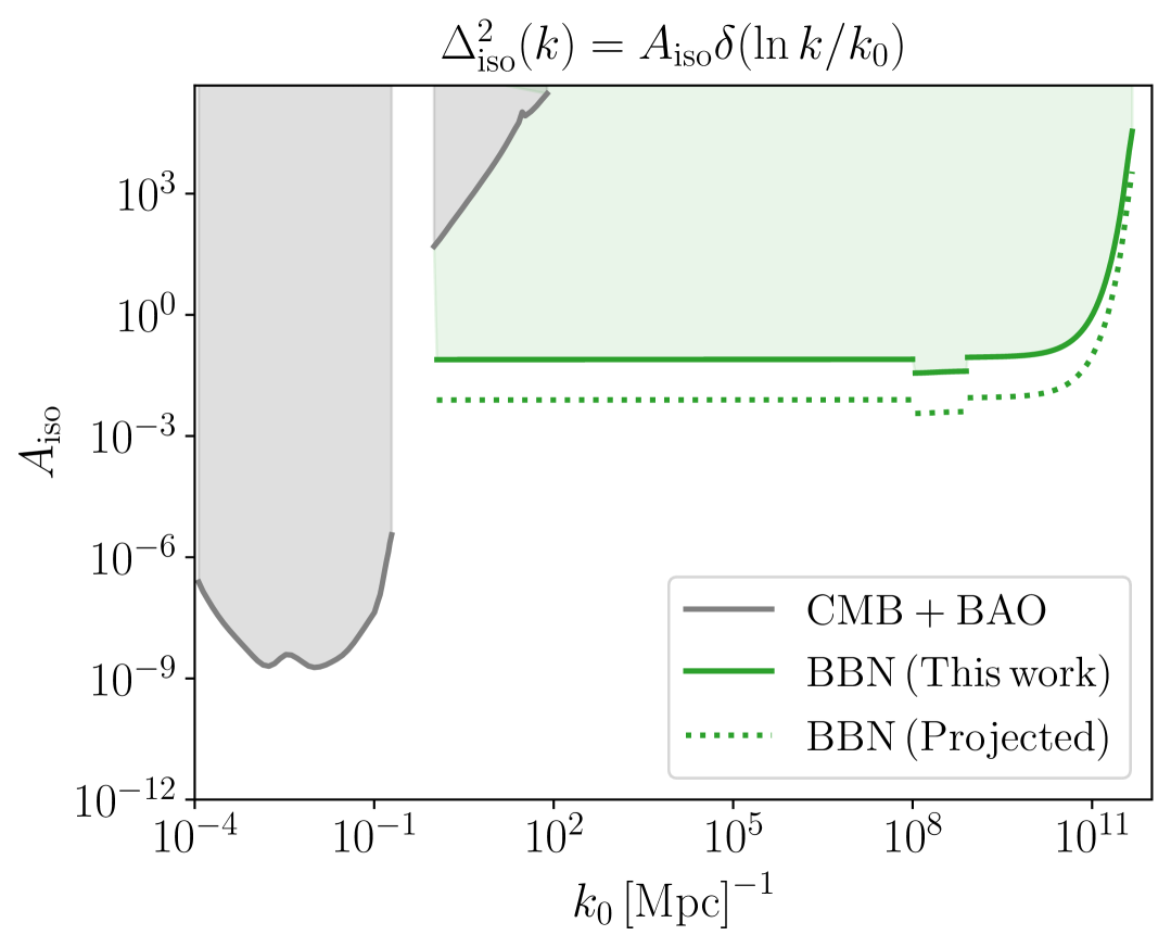
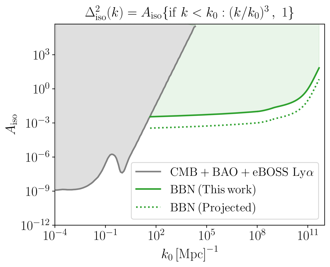
Figure 4: Constraints on inhomogeneities from BBN spanning a wide range of length scales in comparison with existing bounds taken from Buckley:2025zgh . The dotted lines show the potential future reach assuming a factor of $10$ increase in the sensitivity. (Left) A delta function power spectrum of eq. (55). Note the stronger sensitivity of BBN to inhomogeneities in regime (2.a), see eq. (49). In the existing bounds there is a gap, however in that region, bounds coming from the Lyman-$\alpha$ forest are expected to be strong. They were not included in Buckley:2025zgh as they are not within the validity of their approximations. (Right) Broken power law given in eq. (56).

4 Constraints on scenarios that produce baryon inhomogeneities

In this section, we investigate the implications of our novel constraints on various scenarios that lead to inhomogeneities in the baryon-to-photon ratio. We first investigate baryogenesis scenarios that generate an inhomogeneous baryon distribution. Later we turn to models that imprint inhomogeneities on an initially homogeneous universe.

4.1 Constraints on baryogenesis mechanisms

Models that produce baryons at temperatures below the $\mathrm{TeV}$ scale and give rise to sizable inhomogeneities in the baryon-to-photon ratio can be tested by BBN. In the following, we first discuss the important case of electroweak baryogenesis, and then comment on some other recently proposed mechanisms that generate the baryon asymmetry inhomogeneously.

4.1.1 Electroweak baryogenesis

Arguably, the best-motivated target to probe is electroweak baryogenesis, where baryons are produced at the bubble walls during a first-order electroweak phase transition. The resulting baryon distribution is generically inhomogeneous for several reasons. First, key quantities that determine the baryon yield, such as the sphaleron rate and the velocity of the bubble wall, are temperature dependent. Thus, as bubbles expand and the universe cools, the density of baryons they produce will differ. Additionally, inhomogeneous reheating and bubble collisions can introduce further spatial variations in the baryon-to-photon ratio, especially in scenarios with significant supercooling.

The time scale for cosmological first-order phase transition is set by a parameter $\beta^{-1}$, as commonly used in the literature (see e.g. Turner:1992tz ). The characteristic length scale of the inhomogeneities is then set by the typical bubble separation, $\sim v_{w}/\beta$, where $v_{w}\lesssim 1$ is the bubble wall velocity. Given the proton diffusion length obtained in section 2.2, for a phase transition happening at $T\sim 100\,{\rm GeV}$, and for $\beta/H\gtrsim\mathcal{O}(30)$, the bubble separation is small enough that diffusion processes erase inhomogeneities efficiently. Conversely, for $\beta/H\lesssim\mathcal{O}(30)$, the inhomogeneities survive until the epoch of BBN, potentially leaving observable imprints.

We also expect the magnitude of inhomogeneities to be controlled by the parameter $\left(\beta/H\right)^{-1}$, and for small enough $\ \left(\beta/H\right)^{-1}$ to scale linearly with it. The precise sensitivity to this parameter, however, requires a numerical simulation. A detailed study to determine both the magnitude and spatial profile of the baryon fluctuations is left for future work Futurework1 . Nevertheless, our results suggest that BBN may already constrain a considerable portion of the electroweak baryogenesis parameter space, with further improvement possible up to $\beta/H\sim O(30)$. Interestingly, this is the regime of electroweak baryogenesis where the largest gravitational wave signal is produced.

4.1.2 Other baryogenesis scenarios

Any model that produces baryons inhomogeneously at large enough length scales is subject to the BBN constraint. In this section, we briefly discuss two additional baryogenesis scenarios that are in tension with the constraints presented in this work.

First, we comment on a scenario of baryogenesis via domain walls Azzola:2024pzq . In this scenario, the SM is extended by a singlet scalar field that takes different expectation values in different domains, separated by domain walls. These domain walls quickly enter the so-called scaling regime, with only a few domains per Hubble volume. Due to the coupling of the singlet scalar to the SM Higgs, the Higgs vacuum expectation value (VEV) is reduced within the core of the domain wall. Denoting the Higgs expectation value outside the domain wall by $v$ and inside the domain wall core by $v_{\text{core}}$, at temperatures where $v\gg T\gg v_{\text{core}}$, the sphaleron rate inside the wall remains unsuppressed, while outside the wall it is exponentially suppressed. As the domain walls move through space, the baryon asymmetry is generated at the domain wall position, in analogy to electroweak baryogenesis. Since the domain walls move slowly, we expect that baryon production is very inhomogeneous. These inhomogeneities are generated on length scales of $\mathcal{O}(H^{-1})$ at the electroweak epoch and thus persist all the way until BBN. We thus expect this model not to be in agreement with the observed light element abundances.

Another model of baryogenesis that is in conflict with our novel constraints was recently proposed in Elor:2024cea . This model utilizes CP violation from $B$-meson oscillations within the Standard Model as the source of CP violation to generate the baryon asymmetry. The remaining Sakharov conditions are satisfied as follows: $B$-mesons are produced through the out-of-equilibrium decay of some heavy particle into $b$-quarks, and the $B$-mesons subsequently decay into dark-sector states that carry baryon number. This decay is mediated by a heavy particle. In order for the SM CP violation to be sufficient, they need this mediator to be light in the early universe at around $T\sim 100\,\mathrm{MeV}$. However, collider bounds require this mediator to be heavy now. This is achieved by changing its mass at temperatures below $O(100~\mathrm{MeV})$. This variation in mass is achieved via a domain wall network, where the mediator is light in some domains and heavy in others. Consequently, significant baryon asymmetry is generated only in domains where the mediator is light. This leads to large inhomogeneities on length scales that survive until BBN, placing the model in tension with the observed abundances of light elements.

4.2 Correlation with gravitational waves

Our novel constraints are not limited to models that produce baryons inhomogeneously. Inhomogeneities can also be imprinted onto the baryon-to-photon ratio well after baryogenesis has occurred. In particular, models that produce a significant gravitational wave (GW) signal often also generate sizable baryon inhomogeneities at a similar length scale, thereby making them testable through BBN. As we discussed in section 2, the inhomogeneities with a comoving characteristic length scale larger than the proton diffusion length at BBN, survive until then and are tested. Interestingly, the proton diffusion length at BBN corresponds today to a wavelength of $\mathcal{O}(10^{9})\,\rm{km}$ and a frequency $f\sim 0.1\,\rm{mHz}$. On the other hand, the horizon size at BBN corresponds to a frequency $f\sim\rm{pHz}$. One can generically expect that cosmological (pre-BBN) sources that give rise to a large GW background in this frequency range can be probed by BBN. This in particular includes the frequency range of the pulars timing arrays (PTAs) as well as part of the LISA frequency range.

An important source of a stochastic GW background are first-order phase transitions which proceed through nucleation of bubbles. The GW signal from a first-order phase transition is maximized for large bubble separations and large amount of energy density in the bubbles. Such a first-order phase transition not only produces GWs, but also imprints inhomogeneities on the baryon-to-photon ratio, especially if the phase transition is supercooled. This occurs because parts of the space in which bubbles nucleate later experience prolonged expansion leading to adiabatic fluctuations. Moreover, reheating happens inhomogeneously in space which produces fluctuations in the baryon-to-photon ratio. The evolution of both types of modes is discussed in appendix C. We thus expect a correlation between a large GW signal, and inhomogeneities in baryons at large scales. Although we do not discuss a potential first-order QCD phase transition below, we note that in this case, we expect even larger inhomogeneities, as the properties of particles carrying baryon number change drastically between the two phases.

In this section, we first examine inhomogeneities induced by a strong first-order EW phase transition, which could be observable at LISA LISA:2017pwj , followed by a discussion of two scenarios that aim to explain the recently observed PTA signal Xu:2023wog ; NANOGrav:2023gor ; EPTA:2023fyk ; Reardon:2023gzh .

4.2.1 LISA frequency range

A GW signal from a first-order EW phase transition may be within the discovery potential of LISA LISA:2017pwj . For a phase transition happening around $T\simeq 100\rm{GeV}$, LISA is sensitive to $\beta/H\lesssim O(100)$ and strength $\alpha\equiv\frac{\rho_{\text{vac}}}{\rho_{\text{rad}}}\gtrsim O(0.1)$  Caprini:2024hue , where $\rho_{\text{vac}}$ is the energy density of the false vacuum, and $\rho_{\text{rad}}$ the energy density in radiation during the phase transition.

Inhomogeneities are generated on length scales determined by the typical bubble separation which is of order $(H/\beta)\;l_{H}$, thus inhomogeneities produced in a phase transition with $\beta/H=O(30)$ will survive until BBN. We expect the magnitude of the inhomogeneities to be controlled by a combination of $\beta/H$ and $\alpha$, but a precise determination requires a numerical simulation.

Let us, however, estimate the amplitude of inhomogeneities imprinted by a supercooled phase transition with $\alpha\gtrsim 1$. The time it takes for the first bubbles to nucleate until the phase transition is completed is $\delta t\sim O(\text{few})/\beta$. Since the bubbles that nucleate first reheat first and then cool through expansion, we estimate

$$\frac{\Delta T}{T}\sim\frac{O(\text{few})H}{\beta}\,,$$ (57)

while this initially doesn’t produce inhomogeneities in the baryon density itself. This means that one finds inhomogeneities in the baryon-to-photon ratio of order

$$\Delta\eta\simeq 3\frac{\Delta T}{T}\bar{\eta}\simeq O(10)\frac{H}{\beta}\bar{\eta}\,,$$ (58)

where we used $\eta\propto T^{-3}$ and eq. (57). Subsequently, the difference in temperature in the fluid homogenizes. As discussed in appendix C, the homogenization of modes generated at the electroweak scale is under-damped and thus the inhomogeneities in the baryon-to-photon ratio remain. We thus expect equation (58) to also give an estimate of the final inhomogeneities in the baryon density after the fluid has relaxed, but still before the diffusion of baryon number takes place.

This shows the potential reach of BBN to probe first-order phase transitions and calls for a robust study that investigates the magnitude of inhomogeneities that is imprinted on the baryon-to-photon ratio in cases with and without significant supercooling.

4.2.2 Pulsar timing array signal

The GW signal recently observed by PTAs Xu:2023wog ; NANOGrav:2023gor ; EPTA:2023fyk ; Reardon:2023gzh could be explained by a cosmological phase transition, as discussed in NANOGrav:2023hvm and related works. Such a phase transition could take place both in a completely dark sector or in a sector connected to the SM. Typical parameter values consistent with the PTA signal are $\alpha\sim\mathcal{O}(1)$ and $\beta/H\sim\mathcal{O}(10)$ at temperatures $T\sim\mathcal{O}(100~\mathrm{MeV})$.

If such a phase transition is connected to the SM, we expect it to induce inhomogeneities in the baryon-to-photon ratio on length scales of order $1/(10H)$. These fluctuations are dominated by fluctuations in temperature due to different reheating times (see section 4.2.1). As discussed in appendix C, the temperature fluctuations in the fluid subsequently relax and depending on the length scale of the modes, two distinct regimes are possible. For modes for which initially $\lambda_{\nu}k_{\rm phys}\ll 1$, where $\lambda_{\nu}$ is the neutrino mean free path, are under-damped and the inhomogeneities in the baryon-to-photon ratio remain. On the other hand, modes with $\lambda_{\nu}k_{\rm phys}\gtrsim 1$ are strongly damped, and the inhomogeneities in the baryon-to-photon ratio get reduced. Nevertheless, the inhomogeneities that stay in the baryon-to-photon ratio are likely to be in conflict with our constraints, although a dedicated study is required.

Now we comment on the case that such a phase transition is purely in a dark sector, although we first note that this scenario is already in conflict with the recent constraints on $\Delta N_{\rm eff}$ Yeh:2022heq ; ACT:2025tim . We expect the phase transition to induce correlated fluctuations in temperature and baryon density (but not in the baryon-to-photon ratio) (see section 4.2.1), again on length scales of order $1/(10H)$. In this scenario only modes with $\lambda_{\nu}k_{\rm phys}\gtrsim 1$, which are strongly damped, lead to significant inhomogeneities in the baryon-to-photon after the temperature inhomogeneities are damped. This means that one needs to have modes with initial wave-vector $k_{\rm phys}$ satisfying

$$\frac{k_{\rm phys}}{H}\gtrsim\frac{1}{\lambda_{\nu}H}\sim\left(T/T_{\nu}\right)^{3}\,.$$ (59)

Thus, in the case of phase transitions in a purely dark sector, we expect to get constraints from BBN only if the PT happens rather close to the MeV scale, while the latest data prefers a phase transition occurring around $T\sim 100\,{\rm MeV}$.

Another possible explanation involves the collapse of a domain wall (DW) network NANOGrav:2023hvm ; Ferreira:2024eru . Once formed, the DWs enter a scaling regime with a small number of domains per Hubble volume. A small bias in vacuum energy between domains eventually triggers the collapse of the network. To account for the PTA signal, the DW network must disappear around $T\sim 100~\mathrm{MeV}$ and must contribute $\mathcal{O}(0.1)$ of the total energy density prior to collapse. For the collapse to complete in time, the energy bias between domains must also represent a non-negligible fraction of the energy density. The energy density can either be transferred to the visible sector or remain in a purely dark sector. Although again the scenario where the energy density is transferred purely to dark radiation is in strong conflict with the recent constraints on $\Delta N_{\rm eff}$ Yeh:2022heq ; ACT:2025tim . Analogous to first-order phase transitions, if the energy is transferred to the visible sector, the domain collapse leads to inhomogeneities in the baryon-to-photon ratio. While the spatial scales of these inhomogeneities are large enough to survive until BBN, the precise magnitude of the effect requires dedicated numerical simulations, which we leave for future work. On the other hand, if the energy stays in the dark sector, again there are correlated fluctuations in temperature and baryon density (but not in the baryon-to-photon ratio). We therefore expect to get constraints only if the collapse happens close to the MeV scale.

5 Conclusions and outlook

In this paper, we investigated the constraints on baryon inhomogeneities imposed by Big Bang Nucleosynthesis. We demonstrated that the deuterium-to-hydrogen ratio, $(D/H)$, is particularly sensitive to spatial variations in the baryon-to-photon ratio $\eta$. This sensitivity allows BBN to place novel constraints on the amplitude of inhomogeneities in the baryon density at the time of nucleosynthesis.

By studying the diffusion of baryon number, we showed that inhomogeneities with length scale larger than the comoving horizon size in a radiation dominated universe at $T\approx 3\,\rm{TeV}$ survive until BBN. This length scale is set by the proton diffusion length. We considered two main physical regimes, depending on the length scale of inhomogeneity in comparison with the neutron diffusion length by BBN:

• Both neutrons and protons remain inhomogeneous throughout BBN.

• Neutrons homogenize before BBN, while protons do not.

For each regime, we quantified how spatial variations in $\eta$, or in proton number density with fixed neutron density, affect the $D/H$ ratio. Using the PRyMordial code, we numerically evaluated the $D/H$ abundance as a function of the local inhomogeneity amplitude. We then computed the spatially averaged abundance and compared it to observational constraints. Our main findings are: In the regime where both protons and neutrons are inhomogeneous, current measurements of $D/H$ restrict the RMS amplitude of baryon inhomogeneities to be less than $28\%$. If neutrons homogenize before BBN but protons do not, the $D/H$ abundance becomes even more sensitive to local inhomogeneities, leading to a tighter bound of $19\%$ on the RMS amplitude. The improved sensitivity in the second regime is physically intuitive: if neutrons are uniformly distributed, inhomogeneities in proton densities at the time of deuterium freeze-out are larger. The proton density directly controls the efficiency of deuterium destruction, making $D/H$ in this case more sensitive to initial spatial variations in $\eta$. We also discussed a third regime—where neutron diffusion is active during BBN—where neutron diffusion smooth out secondary inhomogeneities generated during BBN. As shown in appendix A, the final result in this case effectively reduces to the case with no neutron diffusion, as neutron diffusion during BBN reintroduces correlations between proton and neutron densities.

We showed that our bounds place important constraints on scenarios that introduce inhomogeneities in the baryon-to-photon ratio. This applies both to scenarios that produce the baryon asymmetry inhomogeneously, as well as to scenarios where inhomogeneities are imprinted on a previously homogeneous baryon-to-photon ratio. Regarding scenarios of baryogenesis, we investigated the potential reach to constrain electroweak baryogenesis. We then discuss two recently proposed scenarios of baryogenesis that are in tension with our bounds. Furthermore, we highlighted the complementarity of our bounds with gravitational wave observations. First-order phase transitions which produce a large gravitational wave signal, also imprint inhomogeneities on the baryon-to-photon ratio. We show that pre-BBN sources that give rise to a large GW signal in the frequency range of $\text{pHz}-0.1\text{mHz}$ can be probed by BBN.

In this paper, we have provided estimates for the reach of this probe for the electroweak phase transition and electroweak baryogenesis as well as scenarios sourcing gravitational waves. Additionally, models that produce primordial black holes tend to generate sizable inhomogeneities. Determining the precise constraints for these scenarios, however, deserve detailed studies which we leave for future work.

Finally, we would like to emphasize the importance of nuclear cross sections for the bounds presented in this work. While sizable improvements in both the measurements of $D/H$ and the CMB determination of $\eta$ are expected in the near future, these can translate to an improvement in our constraint only if the precision of the relevant nuclear rates improves alongside. The most important of these rates are the ones that consume deuterium, in particular $D+D\to T+p$, $D+D\to\,{}^{3}\mathrm{He}+n$ and $D+p\to\,{}^{3}\mathrm{He}+\gamma$. While the recent improvement in precision of the $D+p\to\,{}^{3}\mathrm{He}+\gamma$ rate by the measurement of the LUNA collaboration has led to more accurate theoretical prediction of $D/H$, even more precision is needed to catch up with the expected improvements in the measurements of $D/H$ and $\eta$.

Appendix A Diffusion during BBN

In this appendix, we discuss the role of diffusion during BBN. We begin by examining neutron diffusion and then consider the case of proton diffusion. While protons do not diffuse significantly between neutrino decoupling and the onset of BBN, they begin to diffuse for $T\lesssim 30~\text{keV}$. As we will show, this has only a minor impact on the final light element abundances. Diffusion lengths for protons and neutrons up to the end of BBN are shown in figure 5.

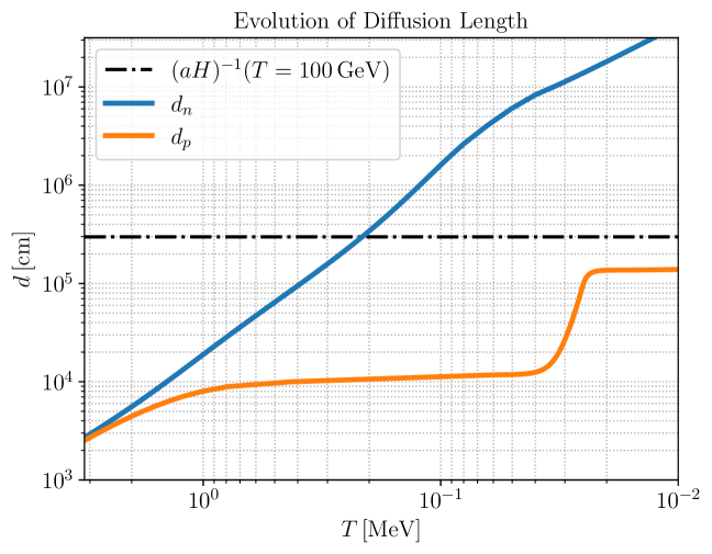
Figure 5: Proton and neutron comoving diffusion lengths up to the end of BBN.

A.1 Neutron diffusion during BBN

Here we are interested in a regime where neutrons diffuse and homogenize, but protons remain inhomogeneous. In this case, BBN proceeds faster in regions with higher proton density. As deuterium forms more efficiently in these regions, neutrons are depleted more quickly and subsequently diffuse to re-establish homogeneity.

We now analyze the case where neutron diffusion is active during BBN. Our goal is to estimate the final proton abundance, starting from an initially inhomogeneous proton distribution and a homogeneous neutron distribution. During BBN, nearly all neutrons are converted into ${}^{4}\mathrm{He}$, primarily via two fusion chains:

$$3p+3n\to 3D\to T+D+p\to{}^{4}\mathrm{He}+p+n\,,$$ (60)

$$3p+3n\to 3D\to D+{}^{3}\mathrm{He}+n\to D+T+p\to{}^{4}\mathrm{He}+p+n\,.$$ (61)

The initial production of deuterium is slow, but once a sufficient amount is formed, subsequent reactions proceed rapidly. Therefore, we can approximate the deuterium, ³He, and tritium densities as being in quasi-equilibrium. The effective reaction that determines the neutron and proton densities is:

$$3n+3p\to{}^{4}\mathrm{He}+n+p\,.$$ (62)

The evolution equations for the comoving neutron and proton densities are then:

$$\partial_{t}n_{n}(x,t) =-\frac{2}{3}\gamma(t)n_{p}(x,t)n_{n}(x,t)+D\nabla^{2}n_{n}(x,t)\,,$$ (63)

$$\partial_{t}n_{p}(x,t) =-\frac{2}{3}\gamma(t)n_{p}(x,t)n_{n}(x,t)\,,$$ (64)

where $\gamma(t)$ sets the deuterium production rate. The factor of $2/3$ accounts for the need to form three deuterium nuclei per ${}^{4}\mathrm{He}$ nucleus (along with a leftover neutron and proton).

Inhomogeneities in proton density enhance reaction rates in overdense regions, which in turn leads to additional neutron diffusion. Thus, to simplify the analysis, we consider the limit $D\gg\gamma n_{p}(x,t)L^{2}$, where $L$ is the characteristic length scale of the inhomogeneities. In this limit the diffusion rate is much faster than the rate of consumption of neutrons by deuterium formation, and therefore we can treat the neutron diffusion as instantaneous:

$$n_{n}(x,t)=n_{n}(t)\,.$$ (65)

Let us consider at some initial time $t_{i}$ just before the onset of helium formation two homogeneous regions with initial proton densities $n_{p}^{+}(t_{i})=\bar{n}_{p}(1+\epsilon)$ and $n_{p}^{-}(t_{i})=\bar{n}_{p}(1-\epsilon)$ where $\bar{n}_{p}$ is the average proton density. Their evolution is governed by

$$\partial_{t}n_{p}^{+}(t) =-\frac{2}{3}\gamma(t)n_{p}^{+}(t)n_{n}(t)\,,$$ (66)

$$\partial_{t}n_{p}^{-}(t) =-\frac{2}{3}\gamma(t)n_{p}^{-}(t)n_{n}(t)\,.$$ (67)

These equations are linear in the proton number densities, and the consumption rate of protons in two regions are equal. Solving these equations gives

$$n_{p}^{+}(t)-n_{p}^{-}(t)=\left(n_{p}^{+}(t_{i})-n_{p}^{-}(t_{i})\right)\exp\left[-\int_{t_{i}}^{t}dt^{\prime}\frac{2}{3}\gamma(t^{\prime})n_{n}(t^{\prime})\right]\,.$$ (68)

To evaluate the exponential factor, we can examine the average proton density

$$\partial_{t}\left(\frac{n_{p}^{+}(t)+n_{p}^{-}(t)}{2}\right)=-\frac{2}{3}\gamma(t)\left(\frac{n_{p}^{+}(t)+n_{p}^{-}(t)}{2}\right)n_{n}(t)\,.$$ (69)

Since protons are mainly depleted through fusion with neutrons, the total difference between proton and neutron numbers is a constant,

$$\frac{n_{p}^{+}(t)+n_{p}^{-}(t)}{2}-n_{n}(t)=c=\text{const}\,.$$ (70)

It is important to note that the constant $c$ is only determined by the space-averaged number densities and is therefore independent of the amount of inhomogeneity in the initial conditions. Now we can plug this back into equation (69) to find

$$\partial_{t}n_{n}(t)=-\frac{2}{3}\gamma(t)\left(c+n_{n}(t)\right)n_{n}(t)\,.$$ (71)

This shows that evolution of the neutron number density in this regime is independent of whether the initial proton distribution is homogeneous or not. We can therefore find it by solving the equations for the homogeneous case. In that case, the proton density evolves as

$$\partial_{t}n_{p}(t)=-\frac{2}{3}\gamma(t)n_{p}(t)n_{n}(t)\,,$$ (72)

with solution

$$n_{p}(t)=n_{p}(t_{i})\exp\left[-\int_{t_{i}}^{t}dt^{\prime}\frac{2}{3}\gamma(t^{\prime})n_{n}(t^{\prime})\right]\,.$$ (73)

The exponential can now be expressed in terms of the proton mass fraction $X_{p}$ as

$$\exp\left[-\int_{t_{i}}^{t}dt^{\prime}\frac{2}{3}\gamma(t^{\prime})n_{n}(t^{\prime})\right]=\frac{X_{p}(T)}{X_{p}(T_{i})}\,,$$ (74)

where $T_{i}\approx 60\,\rm{MeV}$ is the temperature at onset of BBN. If we consider a time $t_{f}$ at the end of helium formation we then have

$$\frac{n_{p}(t_{f})}{n_{p}(t_{i})}=\frac{1-2X_{n}(T_{i})}{1-X_{n}(T_{i})}\,.$$ (75)

Plugging this into eq. (68), we find:

$$n_{p}^{+}(t_{f})-n_{p}^{-}(t_{f})=\left(n_{p}^{+}(t_{i})-n_{p}^{-}(t_{i})\right)\frac{1-2X_{n}(T_{i})}{1-X_{n}(T_{i})}=2\epsilon\,\bar{n}_{p}(t_{i})\frac{1-2X_{n}(T_{i})}{1-X_{n}(T_{i})}\,.$$ (76)

Let’s compare this with the regime where the length scale of inhomogeneities are larger than the neutron diffusion length so that we can consider the inhomogeneities to be correlated and captured by that of $\eta$. In this case the difference in the proton density between the two patches after ${}^{4}\mathrm{He}$ formation is

$$n_{p}^{+}(t_{f})-n_{p}^{-}(t_{f})=\left(n_{p}^{+}(t_{i})-n_{n}^{+}(t_{i})\right)-\left(n_{p}^{-}(t_{i})-n_{n}^{-}(t_{i})\right)=2\epsilon\,\bar{n}_{p}(t_{i})\frac{1-2X_{n}(T_{i})}{1-X_{n}(T_{i})}\,.$$ (77)

Here, the first equality reflects that all neutrons are consumed to form ${}^{4}\mathrm{He}$ in each patch, and the second one uses $\bar{n}_{p}(t_{i})-\bar{n}_{n}(t_{i})=\bar{n}_{p}(t_{i})(1-2X_{n}(T_{i}))/(1-X_{n}(T_{i})$). This demonstrates that, in the limit of fast neutron diffusion, the deuterium abundance remains equally sensitive to baryon inhomogeneities as in the case with no diffusion.

A.2 Proton diffusion during BBN

Following neutrino decoupling, the proton diffusion coefficient remains sufficiently small that proton diffusion is negligible. This remains true until the electron density becomes exponentially suppressed, at which point the proton diffusion coefficient increases rapidly with decreasing temperature. As we will describe now, in this regime, it is the electron diffusion that will eventually slow down the diffusion of protons, as the diffusion of electrons and protons get coupled together to keep charge neutrality. We conclude this section with a discussion on the limited impact of proton diffusion on the final deuterium abundance.

A.2.1 Proton diffusion length during BBN

We begin by describing how electron diffusion eventually limits the diffusion of protons. This happens via the development of an electric potential and subsequently an electric current carried by protons that is comparable to the proton diffusion current. At high temperatures, due to the dense electron-positron plasma, the Coulomb potential is screened on shorter distances. The resulting electric force on protons is negligible, allowing us to treat proton diffusion independently, as done in the main text.

In this subsection we study the evolution of number densities of protons and electrons at short enough length and time scales such that the Hubble expansion can be neglected. The coupled evolution equations for these number densities are (see, e.g., the discussion on ambipolar diffusion in Pitaevskii1981Physical )

$$\frac{\partial\mathfrak{n}_{p}}{\partial t} =D_{p}\left[\nabla^{2}\mathfrak{n}_{p}-\frac{e}{T}\vec{\nabla}\cdot(\vec{E}\,\mathfrak{n}_{p})\right]\,,$$ (78)

$$\frac{\partial\delta\mathfrak{n}_{e}}{\partial t} =D_{e}\left[\nabla^{2}\delta\mathfrak{n}_{e}+\frac{e}{T}\vec{\nabla}\cdot(\vec{E}\,(\mathfrak{n}_{e^{-}}+\mathfrak{n}_{e^{+}}))\right]\,,$$ (79)

where $\delta\mathfrak{n}_{e}=\mathfrak{n}_{e^{-}}-\mathfrak{n}_{e^{+}}$ is the net electron number density, $D_{e}$ is the electron diffusion coefficient, and $\vec{E}$ is the electric field sourced by the charge distribution,

$$\vec{E}=-\vec{\nabla}\phi\qquad\text{with}\qquad\nabla^{2}\phi=-e\left(\mathfrak{n}_{p}-\delta\mathfrak{n}_{e}\right)\,,$$ (80)

where $\Phi$ is the electric potential.

Typically the electron diffusion coefficient is much smaller than the proton diffusion coefficient and is dominated by electron-photon scattering. In eqs. (78) and (79), the first term describes the diffusion of protons and electrons respectively, while the second term describes their reaction to the electric potential. The above equations simplify considerably for approximately homogeneous distributions, as we have $\vec{\nabla}\cdot\left(\vec{E}\,\mathfrak{n}_{p}\right)\simeq\bar{\mathfrak{n}}_{p}\vec{\nabla}\cdot\vec{E}$, and similarly for electrons, where $\bar{\mathfrak{n}}$ describes the mean density. With this approximation, and going to momentum space, we find

$$\frac{\partial\tilde{\mathfrak{n}}_{p}}{\partial t} =D_{p}\left[-k^{2}\tilde{\mathfrak{n}}_{p}-k_{D,p}^{2}(\tilde{\mathfrak{n}}_{p}-\delta\tilde{\mathfrak{n}}_{e})\right]\,,$$ (81)

$$\frac{\partial\delta\tilde{\mathfrak{n}}_{e}}{\partial t} =D_{e}\left[-k^{2}\delta\tilde{\mathfrak{n}}_{e}+k_{D,e}^{2}(\tilde{\mathfrak{n}}_{p}+\delta\tilde{\mathfrak{n}}_{e})\right]\,,$$ (82)

where we have defined $k^{2}_{D,p}\equiv\frac{e^{2}}{T}\bar{\mathfrak{n}}_{p}$ and $k^{2}_{D,e}\equiv\frac{e^{2}}{T}\left(\bar{\mathfrak{n}}_{e^{-}}+\bar{\mathfrak{n}}_{e^{+}}\right)$ as the square of the Debye wave-vector for protons and electrons respectively.

For the length scales of interest, we always have $k\ll k_{D}$ for both protons and electrons. Subtracting the two equations above, we find the following equation governing the evolution of the electric charge density

$$\frac{\partial\left(\tilde{\mathfrak{n}}_{p}-\delta\tilde{\mathfrak{n}}_{e}\right)}{\partial t} =-\left[D_{p}k_{D,p}^{2}+D_{e}k^{2}_{D,e}\right]\left(\tilde{\mathfrak{n}}_{p}-\delta\tilde{\mathfrak{n}}_{e}\right)-\left(D_{p}\tilde{\mathfrak{n}}_{p}-D_{e}\delta\tilde{\mathfrak{n}}_{e}\right)k^{2}\,.$$ (83)

A fluctuation in charge density would be exponential damped over a short time scale $\tau$ of order

$$\tau\sim\left[D_{p}k_{D,p}^{2}+D_{e}k^{2}_{D,e}\right]^{-1}\,.$$ (84)

This continues until the second term in equation (83) becomes non-negligible. At this point there is a residual charge density of order

$$\left(\tilde{\mathfrak{n}}_{p}-\delta\tilde{\mathfrak{n}}_{e}\right)\sim\frac{D_{p}k^{2}}{D_{p}k_{D,p}^{2}+D_{e}k^{2}_{D,e}}\tilde{\mathfrak{n}}_{p}\,,$$ (85)

where we used $D_{p}\gg D_{e}$ and $\tilde{\mathfrak{n}}_{p}\approx\delta\tilde{\mathfrak{n}}_{e}$. This equation shows that the residual electric charge density is much smaller than the separate electron and proton densities. We now consider two different regimes: at high temperatures, the electron density is not yet suppressed which leads to $D_{e}k^{2}_{D,e}\gg D_{p}k^{2}_{D,p}$, while at low temperatures we have $D_{e}k^{2}_{D,e}\ll D_{p}k^{2}_{D,p}$ .

At high temperatures, plugging equation (85) back into the proton diffusion equation (81), we find

$$\frac{\partial\tilde{\mathfrak{n}}_{p}}{\partial t}=-D_{p}k^{2}\tilde{\mathfrak{n}}_{p}\left[1+\mathcal{O}\left(\frac{D_{p}k_{D,p}^{2}}{D_{e}k^{2}_{D,e}}\right)\right].$$ (86)

Thus at high temperatures, the electric force on protons can be neglected and proton diffusion is not affected by that of electrons. This changes once the electron density is small enough such that $D_{e}k^{2}_{D,e}\sim D_{p}k^{2}_{D,p}$.

In the low temperature regime with $D_{e}k^{2}_{D,e}\ll D_{p}k^{2}_{D,p}$, the coupled equations are again simple to analyse: In this case, both terms on the right hand side of the proton diffusion equation (81) are of similar size. As the proton diffusion coefficient is much larger than the electron one, protons quickly approach equilibrium, in which the two terms cancel each other. We thus find

$$\left(\tilde{\mathfrak{n}}_{p}-\delta\tilde{\mathfrak{n}}_{e}\right)\simeq\frac{k^{2}}{k_{D,p}^{2}}\tilde{\mathfrak{n}}_{p}\,.$$ (87)

Plugging this into the electron diffusion equation (82), we get

$$\frac{\partial\delta\tilde{\mathfrak{n}}_{e}}{\partial t}=-D_{e}k^{2}\delta\tilde{\mathfrak{n}}_{e}\left[1+\frac{k_{D,e}^{2}}{k_{D,p}^{2}}\right]\,.$$ (88)

Electrons thus diffuse with an effective diffusion coefficient of

$$D^{\text{eff}}=D_{e}\left[1+\frac{k_{D,e}^{2}}{k_{D,p}^{2}}\right]\,,$$ (89)

As we have $|\tilde{\mathfrak{n}}_{p}-\tilde{\mathfrak{n}}_{e}|\ll\tilde{\mathfrak{n}}_{p}$, the same equations hold for the proton density. Thus due to charge neutrality, also protons diffuse with the same effective diffusion coefficient of (89). In the very low temperature regime, the effective diffusion coefficient saturates at $D^{\text{eff}}=2D_{e}$. Note that in this limit the result is similar to what is found in Pitaevskii1981Physical , with the effective diffusion coefficient becoming twice the smaller of the diffusion coefficients.

At the temperatures of interest, the electron diffusion is dominated by scattering of photons. The diffusion coefficient is given by

$$D_{e}^{-1}=\frac{4\pi^{2}}{45}\sigma_{Th}T^{3},$$ (90)

where $\sigma_{Th}=\frac{8\pi}{3}\frac{\alpha^{2}}{m_{e}^{2}}$ is the cross section of Thomson scattering. The evolution of both the proton and neutron diffusion lengths after the on-set of BBN are shown in figure 6.

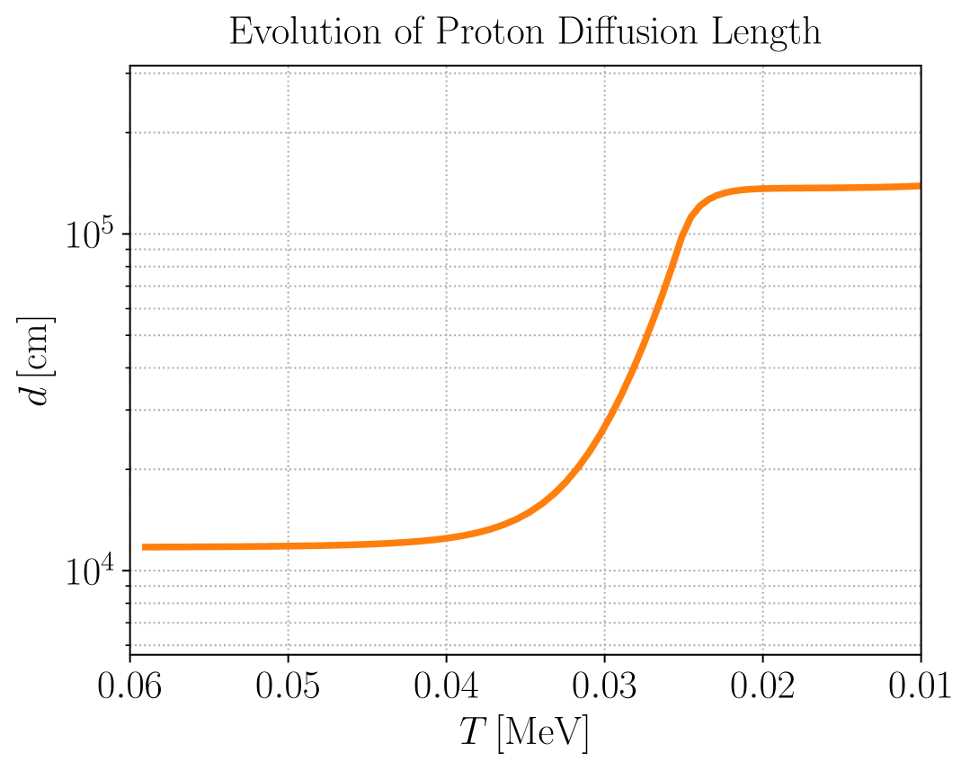
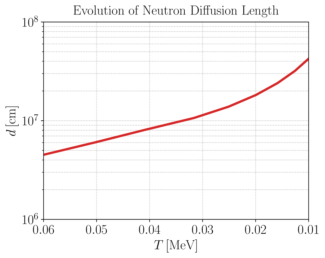
Figure 6: Proton diffusion (Left) and neutron diffusion (Right) during BBN.

A.2.2 Implications of proton diffusion during BBN for deuterium abundance

As can be seen from 6, proton diffusion during BBN is negligible for $T\gtrsim 35\text{keV}$. From that moment until the end of BBN at around $20\text{keV}$, the diffusion length of protons grow by around a factor of six. We now want to estimate the effect of this diffusion on the final deuterium abundance if the length scale of inhomogeneities are within this window.

To obtain an upper bound on the effect of proton diffusion during BBN for such a length scale, we assume that until $35\text{keV}$ protons and deuterium is inhomogeneous, while below $35\text{keV}$ the diffusion coefficient is large and we assume both protons and deuterium are homogenized instantly. After this homogenization, the proton abundance becomes its value in the standard homogeneous BBN, while the deuterium abundance is larger by $O(\langle\epsilon^{2}\rangle)$, just as discussed in the main text.

As discussed below equation (37), the final deuterium abundance is determined by the freeze-out of the rates that destroy deuterium. Below $35\text{keV}$, the abundance of deuterium changes only by around $35\%$. Treating this as a small parameter, one could thus expect changes in the final deuterium abundance, compared to the case where proton diffusion is negligible, of order $0.35\,\epsilon^{2}$, which could be a non-negligible correction to our result. We will now see that the effect is somewhat smaller than that.

The freeze-out of deuterium is governed by the rates $D+D\to T+p$, $D+D\to{}^{3}\mathrm{He}+n$, and $D+p\to\,{}^{3}\mathrm{He}+\gamma$. After all neutrons are eaten up by ${}^{4}\text{He}$, we write the Boltzmann equation for the deuterium abundance as

$$\frac{\partial X_{D}}{\partial t}=-\gamma_{DD}X_{D}^{2}-\gamma_{pD}X_{p}X_{D}\,.$$ (91)

Here $\lambda_{DD}$ describes the rate of the processes involving two deuterium, while $\lambda_{pD}$ describes the rate of the process involving a proton. While both rates are strongly temperature dependent, this dependence is mainly due to the Coulomb barrier and similar for both. The relative size between the two depends mainly on the deuterium fraction at a given temperature. At $T=35\,\text{keV}$, one has $D/H\simeq 3.5\cdot 10^{-5}$, and one finds that the destruction rate through the process involving only deuterium is a factor of around 2 larger than the through the one involving a proton. Thus the destruction of about $1/3$ of the remaining deuterium, which is controlled only by the proton number density, is therefore independent of $\epsilon\,$. As a result, we expect that the final deuterium abundance is corrected by order $2/3\times 0.35\epsilon^{2}\simeq 0.2\epsilon^{2}$ compared to the results of the main text.

We thus conclude that if the inhomogeneities are on large enough length scales such that proton diffusion is negligible until $20~\text{keV}$, the constraints of our main text remain unchanged, while if the inhomogeneities are on smaller scales, the results can be modified by up to $20\%$. In order to quantify this modification as a function of length scales of the inhomogeneities, a combined analysis of BBN and diffusion is necessary, which is left for future work.

Appendix B Toy model for inhomogeneities

In this appendix we present a toy model for the inhomogeneities and following their evolution due to diffusion. We show how the variance of the final fluctuations is determined in terms of the length scale characterizing the initial density profile and the diffusion length.

Consider and initial density profile localized in small regions such that the distance among the regions is much larger than the size of the regions themselves. This can be modeled by an initial density profile, defined over a cubic region of volume $(NL)^{3}$, given by

$$\rho(\vec{r},t=0)=\frac{1}{N^{3}}\sum_{n_{x},n_{y},n_{x}=-N/2}^{N/2}\delta^{3}(\vec{r}-L(n_{x}\hat{x}+n_{y}\hat{z}+n_{z}\hat{z}))\,,$$ (92)

where the sum runs over integer values for $n_{x},n_{y}$ and $n_{z}$, and $N$ is a large integer and we will take its limit to infinity at the end. The normalization has been chosen such that the whole space contains unit charge. With diffusion, at later times this evolves into a density profile

$$\rho(\vec{r},t)=\frac{1}{(\sqrt{2\pi}Nd(t))^{3}}\sum_{\vec{n}}e^{-\frac{(\vec{r}-L\vec{n})}{2d(t)^{2}}}\,.$$ (93)

where $d(t)$ is the diffusion length at time $t$. We are interested in evaluating the RMS fluctuation, $\epsilon_{\text{RMS}}$, given by

$$\epsilon_{\text{RMS}}^{2}=\frac{\langle\rho^{2}\rangle-\langle\rho\rangle^{2}}{\langle\rho\rangle^{2}}$$ (94)

It is easier to compute $\langle\rho^{2}\rangle$ in momentum space,

$$\int d^{3}x\rho^{2}(\vec{r},t)=\int\frac{d^{3}k}{(2\pi)^{3}}|\tilde{\rho}(k,t)|^{2}(\vec{r},t)\,,$$ (95)

where $\tilde{\rho}(k,t)$ denotes the Fourier transform of $\rho(r,t)$,

$$\tilde{\rho}(k,t)=\frac{1}{N^{3}}\sum_{\vec{n}}e^{i\vec{k}.\vec{n}L}e^{-\frac{d(t)^{2}k^{2}}{2}}\,.$$ (96)

We find

$$\epsilon_{\text{RMS}}^{2}=\left(\frac{L}{2\sqrt{\pi}d(t)}\sum_{n=-\infty}^{\infty}e^{-\frac{L^{2}}{4d(t)^{2}}n^{2}}\right)^{3}-1$$ (97)

where in the last step we have taken the limit of infinite $N$ and therefore infinite volume. The result is shown as a function of $L/d$ in figure 7. For large time, and therefore large $d$ the distribution becomes homogeneous and $\epsilon_{\text{RMS}}$ vanishes.

In this example, we considered only the effect of diffusion which is captured by a Gaussian transfer function. In this case the limit $\epsilon_{\text{RMS}}=0.3$ is achieved when $L/d\simeq 3$, and $\epsilon_{\text{RMS}}$ exponentially drops as $L/d$ decreases beyond that. We note, however, that considering the evolution of inhomogeneities in the proton number density, the relevant transfer function obtained in section 2.2 deviates considerably from a simple Gaussian function. In particular it drops slower for momenta larger than $d_{p}^{-1}$. In that case the $\epsilon_{\text{RMS}}$ would be larger for small $L/d$.

Figure 7: RMS fluctuation $\epsilon_{\text{RMS}}$ as a function of $L/d$.

Appendix C Evolution of sub-horizon temperature fluctuations

In this appendix we study the evolution of temperature fluctuations that are sub-horizon. In particular we focus on both adiabatic modes where the baryon-to-photon ratio is homogeneous as well as baryon isocurvature modes where the baryon-to-photon ratio fluctuates. We will see that there are two different regimes for the propagation of these modes, an overdamped regime, in which the baryon-to-photon ratio changes due to the strong damping of the temperature modes, and an oscillatory regime, where, while the modes are still damped and produce heat, the baryon-to-photon ratio is unchanged.

Let us consider the evolution of fluctuations in temperature. The fluctuations generally propagate as sound waves and are damped due to the viscosity as well as the heat diffusion. In the regime we consider, the effect of the viscosities, controlled by the mean free path of the particles strongly coupled to fluid (e.g. photon), can be ignored compared to the heat diffusion which is controlled by the longer mean free path of neutrinos. More explicitly consider the fluid with small fluctuations in velocity, pressure and temperature. The velocity changes in response to the force due to the pressure gradient

$$\rho\partial_{t}\vec{u}=-\vec{\nabla}p$$ (98)

and the pressure changes in response to compression/expansion of the fluid as as well due to the heat diffusion

$$\partial_{t}p=-f(T)\vec{\nabla}\cdot\vec{u}+D(T)\nabla^{2}p$$ (99)

Here $f(T)$ depends on the equation of state of the fluid, and $D(T)$ is the heat diffusion constant. Working in the Fourier space and assuming that the rate of change of $f(T)$ and $D(T)$ are both small compared to the frequency of the modes, this gives the following dispersion relation

$$\omega^{2}=c_{s}^{2}k^{2}-iD(T)\omega k^{2},$$ (100)

where $c_{s}$ is the speed of sound. We thus find

$$\omega=\frac{iD(T)k^{2}}{2}\pm\sqrt{-\frac{D(T)^{2}k^{4}}{4}+c_{s}^{2}k^{2}}.$$ (101)

This dispersion relation has two different regimes: if $D(T)k\gg c_{s}$, the system is dominated by diffusion and strongly damped. On the other hand if $D(T)k\ll c_{s}$, the system is undergoing many oscillations before being damped.

To see the implication of these two regimes for the baryon-to-photon ratio, it is instructive to first study a toy example which captures the physics of this system.

A toy example

Consider a cylinder of length $L$ that is divided to two parts by a frictionless piston. Assume the two sides of the cylinder contain equal number of baryons, which we denote by $N_{B}$ and both sides contain radiation with initial temperatures $T_{1}^{(i)}$ and $T_{2}^{(i)}$. Therefore initially the two sides have equal baryon number densities but different “baryon to photon ratio”. Also we assume that the temperatures are large enough that the pressure from radiation dominates over that of the baryons. The piston allows for transfer of heat but it is impermeable to the baryons. For small temperature differences, the dispersion relation for the position of the piston is similar to that of eq. (101) above.

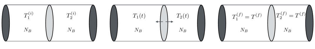
Figure 8: Time evolution of the fluid in the cylinder in the regime of slow heat diffusion (from left to right). The piston between the two fluids oscillates many times around its equilibrium value, before the oscillation is damped. As explained in the text, this does not lead to a change in the baryon-to-photon ratio.

In the limit that the heat transfer is very slow, the piston will oscillate around the point where the pressures (and therefore the temperatures) of the two sides are equal. The oscillations are gradually damped due to heat transfer and the piston eventually relaxes at the equilibrium point. This point is obtained by considering that on each period of oscillation the heat transfer is very small, and on such time scales for each side $j$ we have $T_{j}^{3}V_{j}=\rm{const.}$ where $V_{j}$ is the volume. The piston eventually relaxes at a position $x$ measured from the center of cylinder

$$x=\frac{L}{2}\frac{\left(\frac{T_{1}^{(i)}}{T_{2}^{(i)}}\right)^{1/3}-1}{\left(\frac{T_{1}^{(i)}}{T_{2}^{(i)}}\right)^{1/3}+1}.$$ (102)

Therefore at the end, two sides have different baryon densities. Note that the initial and final baryon to photon ratios for each side is however unchanged. This is because the net heat transfer to each side averages to zero on each oscillation: on half of the oscillation period while $T_{1}>T_{2}$ heat transfers to second part of the cylinder, while in the other half with $T_{2}>T_{1}$, it reverses. This situation is depicted in figure 8, where for concreteness we choose $T_{1}^{(i)}>T_{2}^{(i)}$.

Now instead consider the limit where heat transfer is instantaneous. In this case, the two sides equilibrate without the motion of the piston, leading to the final temperatures being equal and $x=0$. In this limit, the final baryon densities are equal but the baryon to photon ratios are not. This situation is depicted in figure 9. Now if we deviate from this limit by considering smaller heat diffusion, but still in the regime where the oscillations are overdamped, the piston relaxes before reaching the point obtained in equation (102). In this regime, the heat transfer is only from the initially hotter side to other side, and both the final baryon densities as well as the final baryon-to-photon ratios are different.

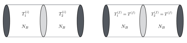
Figure 9: Time evolution of the fluid in the cylinder in the limit of infinite heat diffusion (from left to right). The heat is transferred before the piston starts to move, leading to a change in the baryon-to-photon ratio at both sides of the piston.

Evolution of temperature fluctuations

The above model captures very well the evolution of the fluctuations in the early universe. As we have seen in the main text, baryon diffusion is slow. Also the mean free path of the particles in the plasma (except for the neutrinos) are very small compared to the length scales of interest. These are both modeled by the presence of an impermeable piston in the toy example above. The heat transfer (until neutrino decoupling) is dominantly through neutrinos, which can have a macroscopic mean free path which we denote by $\lambda_{\nu}$. In equation (101) we can then estimate $D\sim\lambda_{\nu}$ and we have $c_{s}^{2}=1/3$ in radiation domination. Therefore the condition for a mode with physical wavenumber $k_{\rm phys}$ to be in the overdamped regime, $D>2c_{s}/k_{\rm phys}$, becomes

$$\lambda_{\nu}k_{\rm phys}\gtrsim 1.$$ (103)

Below the electroweak scale $\lambda_{\nu}$ can be estimated as

$$\lambda_{\nu}\sim\left(G_{F}^{2}T^{5}\right)^{-1},$$ (104)

which is much smaller than the Hubble length scale at high $T$ and becomes of order the Hubble length scale at the time of neutrino decoupling $T_{\nu}\sim\rm{MeV}$. We now consider two distinct examples:

1. The modes are either generated at scale not very far from the horizon size or become sub-horizon at some $T\gg T_{\nu}$.

2. The modes are generated initially with $\lambda_{\nu}k_{\rm phys}\gtrsim 1$.

In case (1), the modes start oscillating and with negligible damping at the beginning. This continues with the amplitudes of the modes gradually falling until a time when $Dk_{\rm phys}^{2}\sim H$, at which point the amplitudes drop significantly. Given that at that moment, the modes are well within the horizon, $k_{\rm phys}\gg H$, it follows that $Dk_{\rm phys}\ll 1$ which means that the modes are still underdamped. So in this case, the baryon-to-photon ratio remains unchanged even after the modes have disappeared.

In case (2), however, the modes start already in the overdamped regime and they disappear without oscillating, leading to a very small change in the baryon density, while the final baryon-to-photon ratio changes.

Finally let us comment on some specific scenarios discussed in the main text. Scenarios where inhomogeneities are produced at the electroweak scale, such as electroweak baryogenesis or a strong first-order electroweak phase transition fall into case (1). In both cases, there are both adiabatic as well as isocurvature modes produced. Inhomogeneities in temperature are damped in a way that the inhomogeneities in the baryon-to-photon ratio remain. This is different for scenarios that happen close to the MeV scale, like phase transitions proposed to explain the PTA signal. If such a phase transition happens purely in a dark sector, it produces inhomogeneities in temperature and the baryon density, but the baryon-to-photon ratio stays homogeneous. If such a phase transition however is coupled to the visible sector, in addition there are inhomogeneities in the baryon-to-photon ratio. For such late phase transitions, depending on the mode, it might well be in scenario (2). In this case these modes are strongly damped, and even the adiabatic modes lead to inhomogeneities in the baryon-to-photon ratio, so to isocurvature modes.

References

- (1) Planck collaboration, Planck 2015 results. XIII. Cosmological parameters, Astron. Astrophys. 594 (2016) A13 [1502.01589].
- (2) Planck collaboration, Planck 2018 results. VI. Cosmological parameters, Astron. Astrophys. 641 (2020) A6 [1807.06209].
- (3) T.-H. Yeh, J. Shelton, K.A. Olive and B.D. Fields, Probing physics beyond the standard model: limits from BBN and the CMB independently and combined, JCAP 10 (2022) 046 [2207.13133].
- (4) V. Mossa et al., The baryon density of the Universe from an improved rate of deuterium burning, Nature 587 (2020) 210.
- (5) Planck collaboration, Planck 2018 results. X. Constraints on inflation, Astron. Astrophys. 641 (2020) A10 [1807.06211].
- (6) K. Inomata, M. Kawasaki and Y. Tada, Revisiting constraints on small scale perturbations from big-bang nucleosynthesis, Phys. Rev. D 94 (2016) 043527 [1605.04646].
- (7) D. Jeong, J. Pradler, J. Chluba and M. Kamionkowski, Silk damping at a redshift of a billion: a new limit on small-scale adiabatic perturbations, Phys. Rev. Lett. 113 (2014) 061301 [1403.3697].
- (8) M.R. Buckley, P. Du, N. Fernandez and M.J. Weikert, General Constraints on Isocurvature from the CMB and Ly- Forest, 2502.20434.
- (9) G. Elor, R. Houtz, S. Ipek and M. Ulloa, The Standard Model CP Violation is Enough, 2408.12647.
- (10) J. Azzola, O. Matsedonskyi and A. Weiler, Minimal Electroweak Baryogenesis via Domain Walls, 2412.10495.
- (11) J.H. Applegate and C.J. Hogan, Relics of Cosmic Quark Condensation, Phys. Rev. D 31 (1985) 3037.
- (12) J.H. Applegate, C.J. Hogan and R.J. Scherrer, Cosmological Baryon Diffusion and Nucleosynthesis, Phys. Rev. D 35 (1987) 1151.
- (13) G.J. Mathews, B.S. Meyer, C.R. Alcock and G.M. Fuller, Coupled Baryon Diffusion and Nucleosynthesis in the Early Universe, APJ 358 (1990) 36.
- (14) H. Kurki-Suonio, M.B. Aufderheide, F. Graziani, G.J. Mathews, B. Banerjee, S.M. Chitre et al., Diffusion coefficients and inhomogeneous big bang nucleosynthesis, Phys. Lett. B 289 (1992) 211.
- (15) I.-S. Suh and G.J. Mathews, Finite temperature effects on cosmological baryon diffusion and inhomogeneous big bang nucleosynthesis, Phys. Rev. D 58 (1998) 123002 [astro-ph/9805179].
- (16) K. Jedamzik and G.M. Fuller, The Evolution of nonlinear subhorizon scale entropy fluctuations in the early universe, Astrophys. J. 423 (1994) 33 [astro-ph/9312063].
- (17) K. Jedamzik, G.M. Fuller and G.J. Mathews, Inhomogeneous primordial nucleosynthesis: Coupled nuclear reactions and hydrodynamic dissipation processes, Astrophys. J. 423 (1994) 50 [astro-ph/9312065].
- (18) A. Heckler and C.J. Hogan, Neutrino heat conduction and inhomogeneities in the early universe, Phys. Rev. D 47 (1993) 4256.
- (19) K. Jedamzik and J.B. Rehm, Inhomogeneous big bang nucleosynthesis: Upper limit on Omega(b) and production of lithium, beryllium, and boron, Phys. Rev. D 64 (2001) 023510 [astro-ph/0101292].
- (20) K. Kainulainen, H. Kurki-Suonio and E. Sihvola, Inhomogeneous big bang nucleosynthesis in light of recent observations, Phys. Rev. D 59 (1999) 083505 [astro-ph/9807098].
- (21) G.M. Fuller, K. Jedamzik, G.J. Mathews and A. Olinto, On Constraining electroweak baryogenesis with primordial nucleosynthesis, Phys. Lett. B 333 (1994) 135 [astro-ph/9407034].
- (22) A.F. Heckler, The Effects of electroweak phase transition dynamics on baryogenesis and primordial nucleosynthesis, Phys. Rev. D 51 (1995) 405 [astro-ph/9407064].
- (23) A. Megevand and F. Astorga, Generation of baryon inhomogeneities in the electroweak phase transition, Phys. Rev. D 71 (2005) 023502 [hep-ph/0409321].
- (24) R.H. Brandenberger, A.-C. Davis and M.J. Rees, Nucleosynthesis constraints on defect mediated electroweak baryogenesis, Phys. Lett. B 349 (1995) 329 [astro-ph/9501040].
- (25) WMAP collaboration, First year Wilkinson Microwave Anisotropy Probe (WMAP) observations: Preliminary maps and basic results, Astrophys. J. Suppl. 148 (2003) 1 [astro-ph/0302207].
- (26) J.D. Barrow and R.J. Scherrer, Constraining Density Fluctuations with Big Bang Nucleosynthesis in the Era of Precision Cosmology, Phys. Rev. D 98 (2018) 043534 [1803.02383].
- (27) K. Inomata, M. Kawasaki, A. Kusenko and L. Yang, Big Bang Nucleosynthesis Constraint on Baryonic Isocurvature Perturbations, JCAP 12 (2018) 003 [1806.00123].
- (28) A.-K. Burns, T.M.P. Tait and M. Valli, PRyMordial: the first three minutes, within and beyond the standard model, Eur. Phys. J. C 84 (2024) 86 [2307.07061].
- (29) V.F. Mukhanov, Nucleosynthesis without a computer, Int. J. Theor. Phys. 43 (2004) 669 [astro-ph/0303073].
- (30) L.P. Pitaevskii and E.M. Lifshitz, Physical Kinetics: Volume 10 (Course of Theoretical Physics), Butterworth-Heinemann (Jan., 1981).
- (31) D. Albornoz Vasquez, A. Belikov, A. Coc, J. Silk and E. Vangioni, Neutron injection during primordial nucleosynthesis alleviates the primordial 7Li problem, Phys. Rev. D 86 (2012) 063501 [1208.0443].
- (32) A. Coc, J.-P. Uzan and E. Vangioni, Mirror matter can alleviate the cosmological lithium problem, Phys. Rev. D 87 (2013) 123530 [1303.1935].
- (33) A. Coc, M. Pospelov, J.-P. Uzan and E. Vangioni, Modified big bang nucleosynthesis with nonstandard neutron sources, Phys. Rev. D 90 (2014) 085018 [1405.1718].
- (34) R.J. Cooke, M. Pettini and C.C. Steidel, One Percent Determination of the Primordial Deuterium Abundance, Astrophys. J. 855 (2018) 102 [1710.11129].
- (35) E.O. Zavarygin, J.K. Webb, V. Dumont and S. Riemer-Sørensen, The primordial deuterium abundance at zabs = 2.504 from a high signal-to-noise spectrum of Q1009+2956, Mon. Not. Roy. Astron. Soc. 477 (2018) 5536 [1706.09512].
- (36) Simons Observatory collaboration, The Simons Observatory: Science goals and forecasts, JCAP 02 (2019) 056 [1808.07445].
- (37) CMB-S4 collaboration, CMB-S4 Science Book, First Edition, 1610.02743.
- (38) R. Cooke, Big Bang Nucleosynthesis, 2409.06015.
- (39) T.-H. Yeh, K.A. Olive and B.D. Fields, The impact of new 3 rates on Big Bang Nucleosynthesis, JCAP 03 (2021) 046 [2011.13874].
- (40) M.S. Turner, E.J. Weinberg and L.M. Widrow, Bubble nucleation in first order inflation and other cosmological phase transitions, Phys. Rev. D 46 (1992) 2384.
- (41) H. Bagherian, M. Ekhterachian and S. Stelzl, Inhomogeneities as a probe of electroweak baryogenesis, work in progress, .
- (42) LISA collaboration, Laser Interferometer Space Antenna, 1702.00786.
- (43) H. Xu et al., Searching for the Nano-Hertz Stochastic Gravitational Wave Background with the Chinese Pulsar Timing Array Data Release I, Res. Astron. Astrophys. 23 (2023) 075024 [2306.16216].
- (44) NANOGrav collaboration, The NANOGrav 15 yr Data Set: Evidence for a Gravitational-wave Background, Astrophys. J. Lett. 951 (2023) L8 [2306.16213].
- (45) EPTA, InPTA: collaboration, The second data release from the European Pulsar Timing Array - III. Search for gravitational wave signals, Astron. Astrophys. 678 (2023) A50 [2306.16214].
- (46) D.J. Reardon et al., Search for an Isotropic Gravitational-wave Background with the Parkes Pulsar Timing Array, Astrophys. J. Lett. 951 (2023) L6 [2306.16215].
- (47) LISA Cosmology Working Group collaboration, Gravitational waves from first-order phase transitions in LISA: reconstruction pipeline and physics interpretation, JCAP 10 (2024) 020 [2403.03723].
- (48) NANOGrav collaboration, The NANOGrav 15 yr Data Set: Search for Signals from New Physics, Astrophys. J. Lett. 951 (2023) L11 [2306.16219].
- (49) ACT collaboration, The Atacama Cosmology Telescope: DR6 Constraints on Extended Cosmological Models, 2503.14454.
- (50) R.Z. Ferreira, A. Notari, O. Pujolàs and F. Rompineve, Collapsing domain wall networks: impact on pulsar timing arrays and primordial black holes, JCAP 06 (2024) 020 [2401.14331].