Pinpointing Triple Point of Noncommutative Matrix Model with Curvature

Abstract

We study a Hermitian matrix model with a quartic potential, modified by a curvature term $\mathrm{tr}(R\Phi^{2})$, where $R$ is a fixed external matrix. Motivated by the truncated Heisenberg algebra formulation of the Grosse-Wulkenhaar model, this term breaks unitary invariance and gives rise to an effective multitrace matrix model via perturbative expansion. We analyze the resulting action analytically and numerically, focusing on the shift of the triple point and suppression of the noncommutative stripe phase—features linked to renormalizability. Our findings, supported by Hamiltonian Monte Carlo simulations, indicate that the curvature term drives the phase structure toward renormalizable behavior by eliminating the stripe phase.

1 Introduction

One promising approach to reconciling the seemingly distinct realms of gravity and quantum theory is modifying the short-distance structure of spacetime Hossenfelder:2012jw . One such modification involves introducing coordinate noncommutativity (NC), initially proposed to incorporate both spacetime symmetries and high-energy cutoffs in quantum field theory (QFT) PhysRev.71.38 .

It is well established that quantum systems in magnetic fields can be described using effective NC coordinates Karabali:2002im ; Karabali:2006eg . Additionally, NC coordinates in principle encode more information than their commutative counterparts Chamseddine:2022rnn . This raises the possibility that the yet unobserved dark matter (DM) might be in fact encoded in NC spacetime. Alternatively, NC could represent a fundamental modification of gravity, which mimics DM in cosmological models through phase transition mechanisms Berezhiani:2015bqa . Furthermore, there are recent hints 10.1093/mnras/staf292 of preferred direction in the observable universe (arguably due to its rotation), which is one of the hallmarks of NC coordinates. Regardless of the interpretation, matrix models provide an ideal framework for studying NC physics due to intrinsic noncommutativity of matrix product and well-defined path integrals.

Matrix models also have extensive applications across various fields, including biophysics, solid-state physics, optics, nuclear physics, and quantum gravity Eynard:2015aea ; Akemann:2011csh ; PhysRevLett.94.168103 ; Beenakker:2014zza ; Weidenmuller:2008vb ; Guhr:1997ve ; Loll:2019rdj . They can serve as a means of regularizing quantum field theories Bietenholz:2014sza and are conjectured to describe fundamental physical laws. In some models, matrix elements function as fields on spacetime, while in others, spacetime itself is absent as an explicit concept. Intriguingly, in certain parameter regimes, spacetime may emerge dynamically within these models Steinacker:2011ix .

A major challenge in NC models is the phenomenon of UV/IR mixing SZABO2003207 , which entangles high- and low-energy scales, thereby complicating renormalization. This mixing disrupts the separation of energy scales—a crucial element of effective field theory Rosaler:2021quv .

Over the past two decades, the Grosse-Wulkenhaar (GW) model Grosse:2003nw ; Grosse:2004yu has successfully addressed the renormalization issues of NC field theories by introducing an additional term in the action, which can be interpreted as arising from curvature of the background NC space Buric:2009ss . We have recently proposed that the nice behavior of the GW model is closely tied to its phase structure, particularly through the suppression of the NC striped phase Prekrat:2021uos ; Prekrat:2022sir . Our results in this regard were obtained using a matrix formulation of the GW model. Further recent exploration of phase structure of different NC matrix models can be found in Gubser:2000cd ; Tekel:2015uza ; Chen:2017kfj ; Kovacik:2018thy ; Han:2019wue ; Kovacik:2020cod ; Ydri:2020efr ; Ydri:2021cam ; Prekrat:2023thesis ; Kovacik:2023zab ; Bukor:2024kqy .

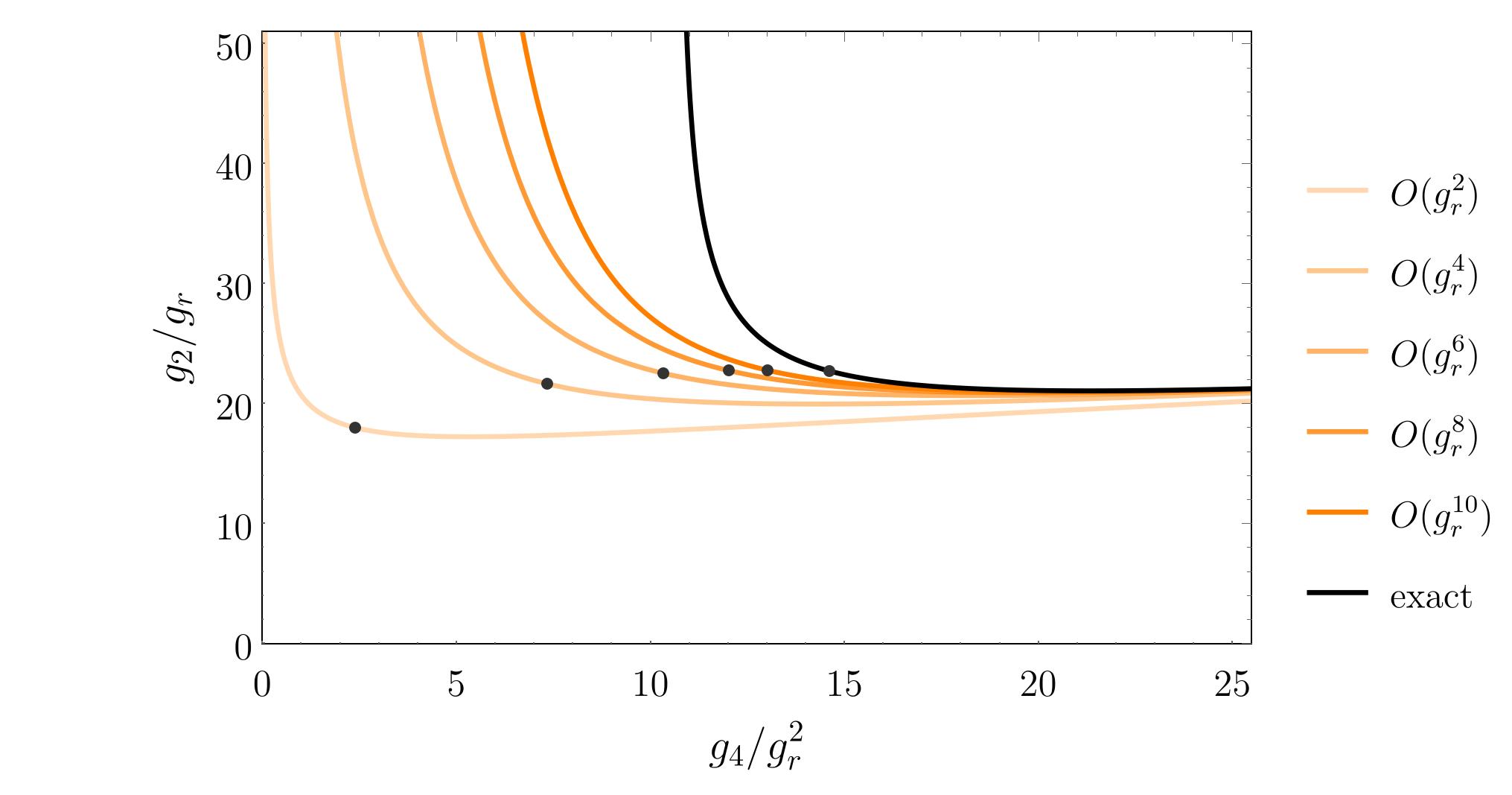
Figure 1: Analytical transition line of the second-order GW model without the kinetic term, shown for different orders of approximation in the curvature coupling $g_{r}$. The dots indicate the “turning points” of each curve, marking the locations of maximum arc curvature.

The immediate motivation for this work was to derive an analytical prediction for the location of the triple point in the GW model using a sequence of perturbative approximations. To simplify the analysis, we considered a model without the kinetic term and used the turning point of the approximate transition line as a proxy for the true triple point.

However, all such approximate transition lines exhibit square-root behavior at large self-coupling and diverge at finite values of the coupling within the perturbative regime—a behavior commonly observed in other multitrace matrix models as well Subjakova:2020gdh .

Interestingly, the turning point of the fourth-order approximation to the transition line derived from the full effective action lies closer to the expected location of the true triple point than the turning point of the exact transition line computed using the second-order effective action Prekrat:2022sir . Furthermore, as shown in Figure 1, successive perturbative approximations to the second-order action transition line exhibit turning points that appear to converge monotonically toward the exact result.

This led us to hope that a similar pattern of convergence might emerge for higher-order approximations based on the full action. However, our analysis up to sixth order in the curvature coupling indicates that such monotonic convergence does not occur—at least not at low perturbative orders.

This paper is organized as follows. In Section 2, we introduce the GW model and present its matrix formulation, emphasizing the role of the curvature term. Section 3 discusses the physical significance of phase transitions in the context of renormalization and highlights the connection between the triple point shift and the suppression of the noncommutative stripe phase. In Section 4, we derive the effective action through a perturbative expansion and obtain analytical expressions for the phase transition lines. Section 5 reviews the underlying matrix model techniques used to analyze eigenvalue distributions and free energy. Section 6 focuses on the phase diagrams of truncated multitrace submodels, while Section 7 presents a detailed comparison with Hamiltonian Monte Carlo (HMC) simulations of the full model. Finally, in Section 8, we summarize our findings and outline future directions for extending this work.

2 GW Model & Matrix Action

We begin by introducing our model and its underlying NC space. The starting point is the two-dimensional GW-model Grosse:2003nw

$$S_{\text{\tiny GW}}=\int\!\!\mathrm{d}^{2}x\,\Bigg{(}\frac{1}{2}\partial^{\mu}\phi\star\partial_{\mu}\phi\;+\;\frac{m^{2}}{2}\phi\star\phi\;+\;\frac{\lambda}{4!}\phi\star\phi\star\phi\star\phi\;+\;\\ \;+\;\frac{\Omega^{2}}{2}((\theta^{-1})_{\mu\rho}x^{\rho}\phi)\star((\theta^{-1})^{\mu\sigma}x_{\sigma}\phi)\Bigg{)}\,,$$ (2.1)

which lives on the Moyal plane equipped with a $\star$-product

$$f\star g=f\,e^{\nicefrac{{\text{i}}}{{2}}\,{\mathchoice{\vbox{\offinterlineskip\halign{#\cr\reflectbox{$\displaystyle\vec{}\mkern 4.0mu$}\cr\kern-3.01389pt\cr$\displaystyle\partial$\cr}}}{\vbox{\offinterlineskip\halign{#\cr\reflectbox{$\textstyle\vec{}\mkern 4.0mu$}\cr\kern-3.01389pt\cr$\textstyle\partial$\cr}}}{\vbox{\offinterlineskip\halign{#\cr\reflectbox{$\scriptstyle\vec{}\mkern 4.0mu$}\cr\kern-2.10971pt\cr$\scriptstyle\partial$\cr}}}{\vbox{\offinterlineskip\halign{#\cr\reflectbox{$\scriptscriptstyle\vec{}\mkern 4.0mu$}\cr\kern-1.50694pt\cr$\scriptscriptstyle\partial$\cr}}}}_{\mu}\theta^{\mu\nu}\vec{\partial}_{\nu}}\,g$$ (2.2)

and with NC coordinates satisfying

$$\commutator{x^{\mu}}{x^{\nu}}_{\star}=\text{i}\theta\epsilon^{\mu\nu}\,.$$ (2.3)

The first line in (2.1) correspond to the standard NC $\lambda\phi^{4}_{\star}$ model, which is non-renormalizable. However, the inclusion of the $\Omega$-term in the second line, renders the model superrenormalizable in two dimensions Wulkenhaar:habilitation2004 .

Applying the Weyl transform and promoting the field $\phi$ to an ${N\times N}$ Hermitian matrix $\Phi$ transforms the action (2.1) into a matrix model

$$S=N\tr\!\left(\Phi\mathcal{K}\Phi-g_{r}R\Phi^{2}-g_{2}\Phi^{2}+g_{4}\Phi^{4}\right)$$ (2.4)

on a background space spanned by NC coordinates

$$X=\frac{1}{\sqrt{2N}}\begin{pmatrix}&\scriptstyle+\sqrt{1}\\ \scriptstyle+\sqrt{1}&&\scriptstyle+\sqrt{2}\\ &\scriptstyle+\sqrt{2}&&\hskip-25.0pt\begin{rotate}{-5.0}{$\ddots$}\end{rotate}\\ &&\hskip-25.0pt\begin{rotate}{-5.0}{$\ddots$}\end{rotate}&&\hskip-16.0pt\scriptstyle+\sqrt{N-1}\\ &&&\hskip-15.0pt\scriptstyle+\sqrt{N-1}&\end{pmatrix}\,,\qquad Y=\frac{\text{i}}{\sqrt{2N}}\begin{pmatrix}&\scriptstyle-\sqrt{1}\\ \scriptstyle+\sqrt{1}&&\scriptstyle-\sqrt{2}\\ &\scriptstyle+\sqrt{2}&&\hskip-25.0pt\begin{rotate}{-5.0}{$\ddots$}\end{rotate}\\ &&\hskip-25.0pt\begin{rotate}{-5.0}{$\ddots$}\end{rotate}&&\hskip-16.0pt\scriptstyle-\sqrt{N-1}\\ &&&\hskip-15.0pt\scriptstyle+\sqrt{N-1}&\end{pmatrix}\,.$$ (2.5)

The price of introducing the finite matrix regularization of the NC coordinates is the modification of their commutation relations (${N\to\infty}$ limit restores the original ones) and curving of the initial Moyal space. The curvature $R$ contains energy levels associated with the $\Omega$-term harmonic oscillator and is given by

$$R=\frac{15}{2N}-8\left(X^{2}+Y^{2}\right)\stackrel{{\scriptstyle\scriptscriptstyle N\gg 1}}{{\approx}}-\frac{16}{N}\operatorname{diag}\left(1,2,\ldots,N\right)\,.$$ (2.6)

The kinetic operator $\mathcal{K}$ is also quadratic in NC coordinates and is defined via double commutators

$$\mathcal{K}\Phi=\commutator{X}{\commutator{X}{\Phi}}+\commutator{Y}{\commutator{Y}{\Phi}}\,.$$ (2.7)

When constructing the model, we included the NC scale $\theta$ in the definitions of the matrix field and the couplings and set it to unity so that we could work with dimensionless quantities. Finally, we also introduce the unscaled versions of couplings

$$G_{2}=Ng_{2}\,,\qquad G_{4}=Ng_{4}\,,$$ (2.8)

as they will appear in the analytical results concerning renormalization.

3 Phase Transitions & Renormalization

In this section, we discuss the significance of the phase transitions for the renormalization properties of the model under study.

The phase diagram of our model illustrates which vacuum solutions are realized across different parameter regimes. Applying the saddle point method to the matrix action (2.4) yields the following equation of motion:

$$2\mathcal{K}\Phi-g_{r}\left(R\Phi+\Phi R\right)+2\Phi\left(2g_{4}\Phi^{2}-g_{2}\!\operatorname{\mathbb{1}}\right)=0\,.$$ (3.9)

This equation has several relevant (approximate) solutions depending on the dominance of the kinetic term ($\mathcal{K}$), curvature term ($R$), or the pure potential terms (involving $g_{2}$ and $g_{4}$):

$$\;\;\Phi=\frac{\tr\Phi}{N}\!\operatorname{\mathbb{1}}\,,\qquad\quad\Phi=\operatorname{\mathbb{0}}\,,\qquad\quad\Phi^{2}=\frac{g_{2}}{2g_{4}}\!\operatorname{\mathbb{1}}\,.$$ (3.10)

The first two solutions correspond to ordered and the disordered vacua, respectively, both of which also appear in commutative models. The third solution, the so-called stripe or matrix vacuum, is unique to the noncommutative setting and features eigenvalues of both signs. This phase breaks translational symmetry and gives rise to spatial modulation of magnetization Castorina:2007za ; Mejia-Diaz:2014lza ; Ambjorn:2002nj . These eigenvalue configurations are visualized in Figure 2, where they are also referred to as 1-cut symmetric (S1), 2-cut (M2, which can be purely symmetric i.e. S2), and 1-cut asymmetric phases (A1).

Figure 2: Eigenvalue distribution $\rho(\lambda)$ in the matrix GW model for representative phases ($N=24$). The left and the right distributions correspond to the disordered and ordered vacua, respectively, both of which also appear in commutative models. The central orange distribution, the so-called stripe (or matrix) vacuum, is unique to the noncommutative model and features eigenvalues of both signs. This phase breaks translational symmetry and leads to a spatial modulation of magnetization.

Figure 3 presents the overall structure of the phase diagram, obtained using HMC simulations Ydri:2015zba ; betancourt2018conceptual . This structure is similar to that found in other fuzzy spaces, such as the fuzzy sphere Kovacik:2018thy . Notably, inclusion of the curvature term shifts the phase boundaries toward larger values of the mass parameter $g_{2}$. This is particularly visible in the displacement of the triple point, $\delta g_{2}^{\text{tp}}$, which we found numerically Prekrat:2021uos to scale proportionally with the curvature coupling $g_{r}$. The resulting suppression of the stripe phase has important consequences for the renormalization of the GW model.

To demonstrate this, let us look at the mass renormalization in the GW model given by Vinas:2014exa

$$\delta m^{2}_{\text{ren}}=\frac{\lambda}{12\pi(1+\Omega^{2})}\ln\frac{\Lambda^{2}\theta}{\Omega}\,,$$ (3.11)

where the matrix size $N$ acts as the UV cutoff via ${\Lambda^{2}\propto N}$ Grosse:2003nw . Using the qualitative correspondences ${m\leftrightarrow G_{2}}$ and ${\Omega\leftrightarrow g_{r}}$ Prekrat:2021uos , the renormalization shift in the matrix model becomes Prekrat:2021uos

$$\delta G_{2}^{\text{ren}}\sim-\ln N\,.$$ (3.12)

This implies that the bare coupling $G_{2}$ must shift by

$$\absolutevalue{\delta G_{2}^{\text{\,ren}}}\sim\ln N$$ (3.13)

to absorb quantum corrections. However, this is smaller than the shift of the triple point:

$$\delta G_{2}^{\text{tp}}=N\delta g_{2}^{\text{tp}}\sim Ng_{r}\,,$$ (3.14)

which is the lowest-most-$g_{2}$ point of the stripe phase (Figure 3). As a result, the bare mass parameter must lie outside the stripe phase (which is responsible for UV/IR mixing), and instead within the disordered phase with a trivial vacuum. The same applies to the renormalized version of the $\lambda\phi^{4}_{\star}$ model (denoted by $\lambda\phi^{4}_{\text{\tiny GW}}$), which is obtained Grosse:2003nw ; Wulkenhaar:habilitation2004 as the limit of a sequence of GW models where the curvature coupling vanishes like

$$\Omega\sim\frac{1}{\ln N}\to 0\,.$$ (3.15)

Further discussion on this topic can be found in Prekrat:2023fts . In contrast, this protective shift does not occur in the original nonrenormalizable $\lambda\phi^{4}_{\star}$ model without the curvature term, whose triple point remains fixed at the origin in the large $N$ limit Prekrat:2021uos , as seen in the ${g_{r}=0}$ plot in Figure 3.

It is also worth noting that changes to the kinetic term can induce similar shifts in the triple point position Subjakova:2020shi and potentially resolve UV/IR mixing issues Dolan:2001gn .

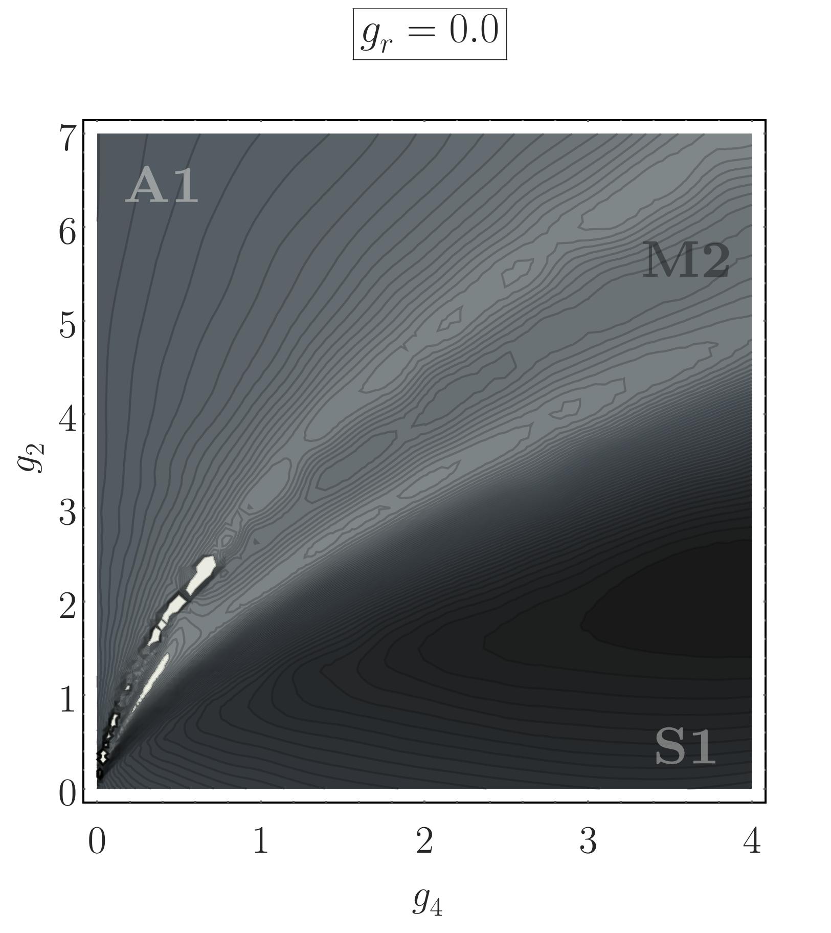
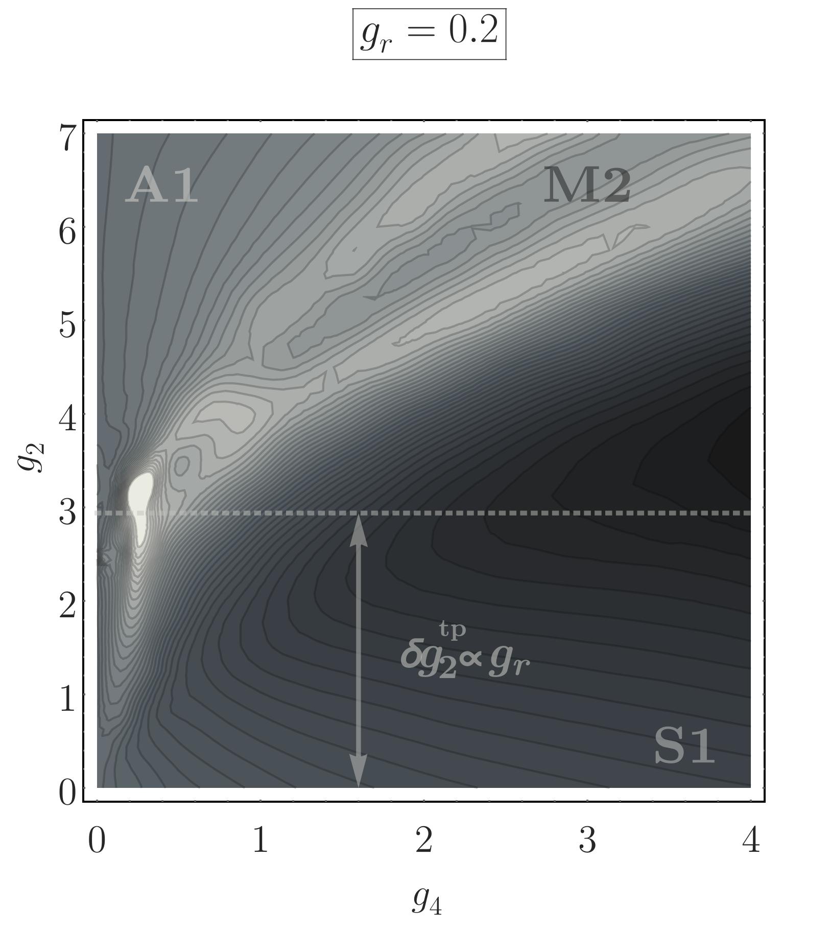
Figure 3: Phase diagrams of the $N=24$ matrix GW model with (right panel) and without (left panel) the curvature term. Darker regions indicate lower specific heat values, while lighter regions indicate higher values. The bright stripes mark the transition lines between phases, with phase labels (abbreviations) shown in the plot corners. Note that the triple point in the right-hand plot is shifted by ${\delta g_{2}^{\text{tp}}\approx 16g_{r}=16\cdot 0.2=3.2}$ relative to the left-hand plot.

4 Effective Action & Transition Lines

Since the link between the GW model’s renormalizability and the suppression of the stripe phase hinges on a numerically observed shift in the phase diagram, it is important to confirm this shift analytically. Initial steps toward this goal were made in Prekrat:2022sir , where the effective action up to $O(g_{r}^{4})$ and the transition line between the disordered and stripe phases were derived for the GW model without the kinetic term.

As shown in Prekrat:2022sir , the approximate analytical transition lines agree well with numerical data in the strong coupling regime. However, a more precise determination of the starting point (the triple point) requires higher-order approximations. In particular, we need to compare different perturbative orders of the effective action to verify whether the turning points of these transition lines converge in the perturbative regime. For this purpose, we derive the $O(g_{r}^{6})$ effective action in this section.

To outline the approach, we recall from Figure 2 that the phase structure depends solely on the distribution of eigenvalues of the matrix field. Hence, we must integrate out the non-eigenvalue (angular) degrees of freedom to obtain the effective action. Starting with the decomposition ${\Phi=U\Lambda U^{\dagger}}$ where $\Lambda$ is diagonal matrix of field eigenvalues and $U$ is unitary matrix, the action becomes:

$$S=N\tr\!\quantity((U\Lambda U^{\dagger})\mathcal{K}(U\Lambda U^{\dagger})-g_{r}RU\Lambda^{2}U^{\dagger}-g_{2}\Lambda^{2}+g_{4}\Lambda^{4})\,.$$ (4.16)

However, the integration over the unitary group is analytically intractable in full generality. Since the shift of the triple point arises solely from the curvature term, we simplify our analysis by neglecting the kinetic term. This approximation is supported by numerical evidence: near the triple point, the eigenvalue distribution closely follows the configuration

$$\Phi^{2}_{R}=\frac{g_{2}\!\operatorname{\mathbb{1}}\!+g_{r}R}{2g_{4}}\,,$$ (4.17)

which solves the equation of motion (3.9) without the kinetic term. The domain of existence of this solution imposes a lower bound on the triple point:

$$g_{2}^{\text{tp}}\geq 16g_{r}\,.$$ (4.18)

Conversely, replacing $R$ by its extremal eigenvalues provides an upper bound Prekrat:2020ptq :

$$g_{2}^{\text{tp}}\leq 16g_{r}\,,$$ (4.19)

yielding the exact location:

$$g_{2}^{\text{tp}}=16g_{r}\,.$$ (4.20)

Numerical simulations confirm that both bounds are saturated.

With the kinetic term neglected, we compute the effective action from the partition function:

$$Z=\int[\mathrm{d}\Phi]\,e^{-S}=\int[\mathrm{d}\Lambda]\,\Delta^{\!2}\!(\Lambda)\,e^{-N\tr\left(-g_{2}\Lambda^{2}+g_{4}\Lambda^{4}\right)}\int[\mathrm{d}U]\,e^{\,g_{r}N\tr\left(URU^{\dagger}\Lambda^{2}\right)}\,,$$ (4.21)

where $\Delta(\Lambda)$ is the Vandermonde determinant:

$$\Delta(\Lambda)=\prod_{1\leq i<j\leq N}\!\!\!(\lambda_{j}-\lambda_{i})\,,\qquad\Lambda=\operatorname{diag}\lambda_{i}\,.$$ (4.22)

To compute the unitary integral, we consider the general case:

$$I=\int\limits_{{\rm U}(N)}\!\![\mathrm{d}U]\,e^{t\tr(UAU^{\dagger}B)}$$ (4.23)

for Hermitian matrices $A$ and $B$, with a normalized Haar measure.

This integral defines corrections $\delta S$ to the effective action:

$$S_{\text{eff}}=-g_{2}N\tr\!\Lambda^{2}+g_{4}N\tr\!\Lambda^{4}-\ln\Delta^{2}(\Lambda)+\delta S\,,$$ (4.24)

where

$$I=\exp\quantity(-\delta S)=\exp\quantity(-\sum_{n=1}^{\infty}\frac{t^{n}}{n!}S_{n})\,.$$ (4.25)

Using the expansion:

$$I=1+\sum_{n=1}^{\infty}\frac{t^{n}}{n!}\,I_{n}\,,\qquad I_{n}=\int[\mathrm{d}U]\tr^{n}\!\quantity(UAU^{\dagger}B)\,,$$ (4.26)

we obtain first few recursive formulas for $S_{n}$:

$$S_{1} =-I_{1}\,,$$ (4.27)

$$S_{2} =S_{1}^{2}-I_{2}\,,$$ (4.28)

$$S_{3} =-S_{1}^{3}+3S_{1}S_{2}-I_{3}\,,$$ (4.29)

$$S_{4} =S_{1}^{4}-6S_{1}^{2}S_{2}+3S_{2}^{2}+4S_{1}S_{3}-I_{4}\,,$$ (4.30)

$$S_{5} =-S_{1}^{5}+10S_{1}^{3}S_{2}-10S_{1}^{2}S_{3}-15S_{1}S_{2}^{2}+5S_{1}S_{4}+10S_{2}S_{3}-I_{5}\,,$$ (4.31)

and

$$\,S_{6}=S_{1}^{6}-15S_{1}^{4}S_{2}+45S_{1}^{2}S_{2}^{2}-15S_{2}^{3}+20S_{1}^{3}S_{3}-60S_{1}S_{2}S_{3}\,+\\ +10S_{3}^{2}-15S_{1}^{2}S_{4}+15S_{2}S_{4}+6S_{1}S_{5}-I_{6}\,.\,$$ (4.32)

In Prekrat:2024rmq , we found $S_{n}$ and $I_{n}$ up to the 6th order with the help of the RTNI computing package Fukuda:2019pzs . We also proved that all odd orders of $S_{n}$ disappear, due to equidistant eigenvalues of the curvature and its symmetry w.r.t. the anti-diagonal. The resulting effective action up to $O(g_{r}^{6})$ is:

$$S_{\text{eff}}= -\quantity(g_{2}-8g_{r})N\tr\!\Lambda^{2}+\quantity(g_{4}-\frac{32}{3}g_{r}^{2})N\tr\!\Lambda^{4}+\frac{32}{3}g_{r}^{2}\tr^{2}\!\!\Lambda^{2}$$ (4.33)

$$+\frac{1024}{45}g_{r}^{4}N\tr\!\Lambda^{8}+\frac{1024}{15}g_{r}^{4}\tr^{2}\!\!\Lambda^{4}-\frac{4096}{45}g_{r}^{4}\tr\!\Lambda^{6}\tr\!\Lambda^{2}\hskip 18.0pt$$

$$-\frac{262144}{2835}g_{r}^{6}N\tr\!\Lambda^{12}+\frac{524288}{945}g_{r}^{6}\tr\!\Lambda^{2}\tr\!\Lambda^{10}-\frac{262144}{189}g_{r}^{6}\tr\!\Lambda^{4}\tr\!\Lambda^{8}+\frac{524288}{567}g_{r}^{6}\tr^{2}\!\!\Lambda^{6}$$

$$-\ln\Delta^{2}(\Lambda)\,.$$

Alternatively, writing this in powers of mass-shift parameter $8g_{r}$ (normalized trace of the curvature), the expansion becomes even more transparent:

$$S_{\text{eff}}= -\quantity(g_{2}-8g_{r})N\tr\!\Lambda^{2}+\quantity(g_{4}-\frac{1}{6}(8g_{r})^{2})N\tr\!\Lambda^{4}+\frac{1}{6}(8g_{r})^{2}\tr^{2}\!\!\Lambda^{2}$$ (4.34)

$$+\frac{1}{180}(8g_{r})^{4}N\tr\!\Lambda^{8}+\frac{1}{60}(8g_{r})^{4}\tr^{2}\!\!\Lambda^{4}-\frac{1}{45}(8g_{r})^{4}\tr\!\Lambda^{6}\tr\!\Lambda^{2}\hskip 18.0pt$$

$$-\frac{1}{2835}(8g_{r})^{6}N\tr\!\Lambda^{12}+\frac{2}{945}(8g_{r})^{6}\tr\!\Lambda^{2}\tr\!\Lambda^{10}-\frac{1}{189}(8g_{r})^{6}\tr\!\Lambda^{4}\tr\!\Lambda^{8}+\frac{2}{567}(8g_{r})^{6}\tr^{2}\!\!\Lambda^{6}$$

$$-\ln\Delta^{2}(\Lambda)\,.$$

This effective action can now be used to derive the eigenvalue distribution and determine the corrections to the phase transition lines, leading to the better analytical estimation of the shift of the triple point. We apply three strategies to extract physical predictions:

1. Analytical expansion of the $N\to\infty$ transition lines in powers of $g_{r}$, using the derived effective action.

2. Numerical analysis of the continuum limit of multitrace matrix models corresponding to the effective action truncated at finite order in $g_{r}$.

3. HMC simulations of the full action to locate the transition line for finite $N$, followed by extrapolation to $N\to\infty$.

Skipping ahead to the results, we list the analytical transition lines up to $O(g_{r}^{6})$:

• Transition from S1 to S2 phase:

  $$g_{2}=2\sqrt{g_{4}}+8g_{r}+\frac{32}{3}\frac{g_{r}^{2}}{\sqrt{g_{4}}}+\frac{256}{15}\frac{g_{r}^{4}}{g_{4}\sqrt{g_{4}}}-\frac{4096}{21}\frac{g_{r}^{6}}{g_{4}^{2}\sqrt{g_{4}}}\,.$$ (4.35)

• (Unrealized) transition from S2 to A1 phase:

  $$g_{2}=\sqrt{15}\sqrt{g_{4}}+8g_{r}+\frac{592}{9\sqrt{15}}\frac{g_{r}^{2}}{\sqrt{g_{4}}}-\frac{503168}{1125\sqrt{15}}\frac{g_{r}^{4}}{g_{4}\sqrt{g_{4}}}+\frac{1581033472}{212625\sqrt{15}}\frac{g_{r}^{6}}{g_{4}^{2}\sqrt{g_{4}}}\,.$$ (4.36)

To simplify, we define dimensionless deformation parameters (relative to the ${g_{r}=0}$ transition lines):

$$\epsilon=\frac{8g_{r}}{2\sqrt{g_{4}}}\ ,\qquad\bar{\epsilon}=\frac{8g_{r}}{\sqrt{15g_{4}}}\ ,$$ (4.37)

so that the above become:

• Transition from S1 to S2 phase:

  $$\frac{g_{2}}{2\sqrt{g_{4}}}=1+\epsilon+\frac{1}{3}\epsilon^{2}+\frac{1}{30}\epsilon^{4}-\frac{1}{42}\epsilon^{6}\,.$$ (4.38)

• (Unrealized) transition from S2 to A1 phase:

  $$\frac{g_{2}}{\sqrt{15g_{4}}}=1+\bar{\epsilon}+\frac{37}{36}\bar{\epsilon}^{2}-\frac{3931}{2400}\bar{\epsilon}^{4}+\frac{771989}{120960}\bar{\epsilon}^{6}\,.$$ (4.39)

The analytical transition lines, alongside the HMC results, are presented in Figure 4. However, these expressions alone do not suffice to accurately pinpoint the location of the triple point. This limitation is evident in Figure 5, where the turning points of the second-, fourth-, and sixth-order approximations to the S1/S2 transition line (4.35) exhibit erratic behavior, “jumping around” rather than converging monotonically to a single point. Moreover, these points deviate from the anticipated triple point position at ${(g_{4},g_{2})=(0,16g_{r})}$. Consequently, any convergence can only be inferred by analyzing higher-order approximations. The same holds for the turning points of the would-be S2/A1 transition line.

We conclude the section by noting that analogous expansion techniques have been initiated for the kinetic term’s contribution to the effective action Benedek:2023stconf . The first nontrivial terms of this expansion are:

$$S_{\text{eff}}^{\text{kin}}=N\tr\!\Lambda^{2}-\tr^{2}\!\!\Lambda+\frac{97}{120}N\tr\!\Lambda^{4}-\frac{565}{120N^{2}}\tr^{4}\!\!\Lambda\,+\\ +\frac{113}{12N}\tr^{2}\!\!\Lambda\tr\!\Lambda^{2}-\frac{137}{60}\tr^{2}\!\!\Lambda^{2}-\frac{97}{30}\tr\!\Lambda\tr\!\Lambda^{3}\,,$$ (4.40)

and will be explored in future work.

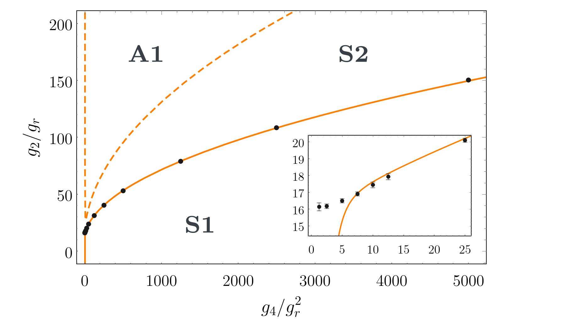
Figure 4: Phase transition lines obtained from the sixth-order effective action. Black dots show HMC simulation results for the full model at $g_{r}=0.02$, extrapolated to the $N\to\infty$ limit. The dashed line denotes the S2–A1 transition, which does not occur in this model.

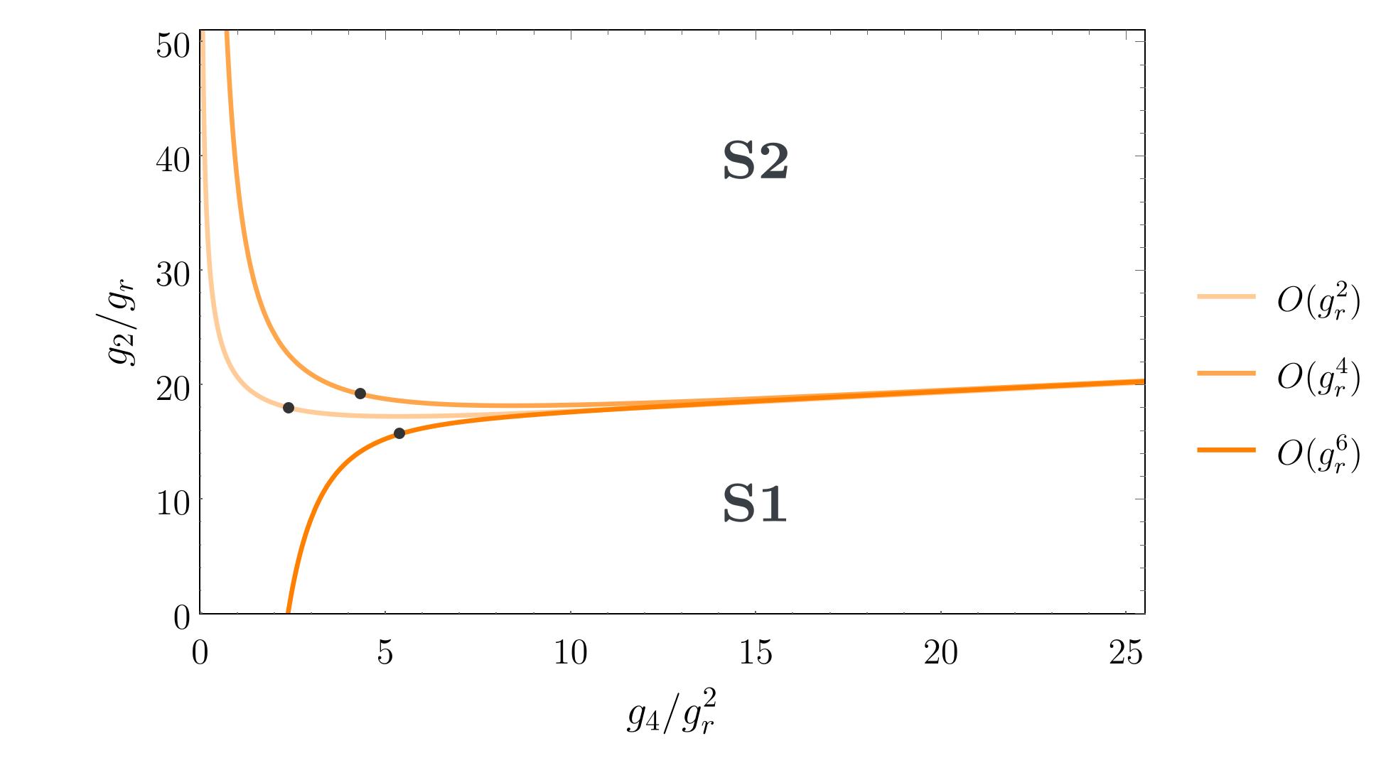
Figure 5: Comparison of the turning points predicted by the second-, fourth-, and sixth-order approximations to the exact S1–S2 transition line (4.35) of the model.

We will now provide a detailed explanation of the three aforementioned strategies employed to obtain our results.

5 Review of the Matrix Model Description

5.1 Eigenvalue Distribution

The phase transitions observed in our model are associated with topological changes in the support of the eigenvalue distribution. To study these transitions, we first derive the eigenvalue distribution for matrix models.

We consider ${N\times N}$ Hermitian matrices with the Dyson integration measure $[\mathrm{d}\Phi]$, and define the probability measure as $e^{-N^{2}\mathcal{S}(\Phi)}$. In this section, for convenience, we work with a rescaled action $\mathcal{S}$, specifically, ${\mathcal{S}=O(1)}$ while previously ${\mathcal{S}=O(N^{2})}$. We also consider a more general form of the potential $V(\Phi)$. The expectation value of a function $f(\Phi)$ is then computed via the partition function (4.21):

$$\left\langle f\right\rangle\,=\,\frac{1}{Z}\int[\mathrm{d}\Phi]e^{-N^{2}\mathcal{S}(\Phi)}f(\Phi)\ ,\qquad Z\,=\,\int[\mathrm{d}\Phi]e^{-N^{2}\mathcal{S}(\Phi)}\ .$$ (5.41)

The most general single-trace action can be written as:

$$\mathcal{S}(\Phi)\,=\,\frac{1}{N}\tr V(\Phi)\,,\qquad V(\Phi)\,=\,\sum_{n=0}^{N}g_{n}\,\Phi^{n},\qquad g_{n}\in\mathds{R}\ .$$ (5.42)

Here, the $1/N$ factor ensures that $\mathcal{S}(\Phi)$ remains of order one when the trace is taken. Upon diagonalizing the Hermitian matrix $\Phi$, we write ${\Phi=U\Lambda U^{{\dagger}}}$, where $\Lambda=\operatorname{diag}\lambda_{i}$ contains eigenvalues $\Phi$ and ${U\in\text{U}(N)}$. The Jacobian of this transformation introduces the aforementioned Vandermonde determinant (4.22):

$$[\mathrm{d}\Phi]=[\mathrm{d}U]\left(\prod_{i=1}^{N}\mathrm{d}\lambda_{i}\right)\left(\prod_{i<j}\left(\lambda_{i}-\lambda_{j}\right)^{2}\right)\,.$$ (5.43)

Assuming ${f(\Phi)}$ is invariant under unitary conjugation (i.e. depends only on eigenvalues), the integral with respect to the Haar measure $[\mathrm{d}U]$ becomes trivial, and the expectation value reduces to:

$$\left\langle f\right\rangle\,=\,\frac{1}{Z}\int\left(\prod_{i=1}^{N}\mathrm{d}\lambda_{i}\right)\exp\left(-N^{2}\left[\mathcal{S}(\Lambda)-\frac{2}{N^{2}}\sum\limits_{i<j}\text{ln}\lvert\lambda_{i}-\lambda_{j}\rvert\right]\right)f(\lambda_{i})\,.$$ (5.44)

We define the quantity in square brackets as the free energy Tekel:2015uza :

$$\mathcal{F}\,=\,\mathcal{S}(\Lambda)-\frac{2}{N^{2}}\sum_{i<j}\text{ln}\lvert\lambda_{i}-\lambda_{j}\rvert\,.$$ (5.45)

From this point onward, we focus exclusively on the continuum limit ${N\rightarrow\infty}$, where the theory becomes more amenable to analytical treatment. In the large-$N$ limit, only the configuration of eigenvalues $\widetilde{\lambda}_{i}$ that globally minimizes $\mathcal{F}$ significantly contributes. This leads to the saddle point equation for the singletrace action (5.42):

$$V^{\prime}(\widetilde{\lambda}_{i})-\frac{2}{N}\sum_{j\neq i}\frac{1}{\widetilde{\lambda}_{i}-\widetilde{\lambda}_{j}}\,=\,0\,.$$ (5.46)

This equation describes the equilibrium of repulsive eigenvalue “particles” in an external potential $V(\Phi)$. To analyze the system further, we define:

• The eigenvalue density:

  $$\rho(\lambda)=\frac{1}{N}\sum_{i=1}^{N}\delta\left(\lambda-\widetilde{\lambda}_{i}\right)\,.$$ (5.47)

• The resolvent:

  $$\omega(z)=\frac{1}{N}\sum_{i=1}^{N}\frac{1}{z-\widetilde{\lambda}_{i}}\,.$$ (5.48)

• The distribution moments:

  $$c_{n}=\frac{1}{N}\tr\Phi^{n}\,.$$ (5.49)

In the $N\to\infty$ limit, the stable configuration $\widetilde{\lambda}_{i}$ becomes continuous distribution function $\rho(\lambda)$ and sums become integrals:

$$\lim_{N\rightarrow\infty}\frac{1}{N}\sum_{i=1}^{N}f(\tilde{\lambda}_{i})\longrightarrow\int_{\mathcal{C}}\mathrm{d}\lambda^{\prime}\,\rho(\lambda^{\prime})\,f(\lambda^{\prime})\,,$$ (5.50)

where $\mathcal{C}$ is the support of the distribution. The resolvent and moments become:

$$\omega(z)\,=\,\int_{\mathcal{C}}\mathrm{d}\lambda^{\prime}\,\frac{\rho(\lambda^{\prime})}{z-\lambda^{\prime}}\,,\qquad\qquad c_{n}=\int_{\mathcal{C}}\mathrm{d}\lambda^{\prime}\,\rho(\lambda^{\prime})\lambda^{\prime n}\,.$$ (5.51)

The saddle point equation (5.46) transforms into the singular integral equation:

$$V^{\prime}(\lambda)-2\cdot\principalvalue\!\int_{\mathcal{C}}\mathrm{d}\lambda^{\prime}\,\frac{\rho(\lambda^{\prime})}{\lambda-\lambda^{\prime}}\,=\,0\,,$$ (5.52)

where $\principalvalue$ denotes the principal value. Using the Sokhotski–Plemelj formula: Tekel:2015uza ,

$$\principalvalue\int_{\mathcal{C}}\mathrm{d}\lambda^{\prime}\,\frac{\rho(\lambda^{\prime})}{\lambda-\lambda^{\prime}}\,=\,\lim_{\varepsilon\rightarrow 0^{+}}\left[\omega(\lambda\pm\text{i}\varepsilon)\pm\text{i}\pi\rho(\lambda)\right]\,,$$ (5.53)

we express (5.52) and $\rho(\lambda)$ as:

$$V^{\prime}(\lambda)\,=\,\lim_{\varepsilon\rightarrow 0^{+}}\left[\omega(\lambda+\text{i}\varepsilon)+\omega(\lambda-\text{i}\varepsilon)\right]\,,$$ (5.54)

$$\rho(\lambda)\,=\,\frac{1}{2\pi\text{i}}\,\lim_{\varepsilon\rightarrow 0^{+}}\left[\omega(\lambda+\text{i}\varepsilon)-\omega(\lambda-\text{i}\varepsilon)\right]\,.$$ (5.55)

Squaring the resolvent, neglecting all the subdominant terms and employing the saddle point equation, one finds a quadratic equation with general solution:

$$\omega(z)=\frac{1}{2}\left[V^{\prime}(z)-\lvert H(z)\rvert\sqrt{\sigma(z)}\right]\,.$$ (5.56)

Here, $\sigma(z)$ is an even polynomial whose roots determine the support $\mathcal{C}$, while $\lvert H(z)\rvert$ is a positive, analytic function and does not contribute to the discontinuity.

We focus on three typical cases of eigenvalue support:

• Symmetric 1-cut (S1):

  $$\sigma_{\text{S1}}(\lambda)=\prod_{\pm}\left(\lambda\pm\sqrt{\delta}\right)\,,\qquad\mathcal{C}_{\text{S1}}=\left(-\sqrt{\delta}\,,\,\sqrt{\delta}\,\right)\,.$$ (5.57)

• Symmetric 2-cut (S2):
  

  $$\sigma_{\text{S2}}(\lambda)=\prod_{\pm,\pm}\left(\lambda\pm\sqrt{D\pm\delta}\right)\,,\\ \mathcal{C}_{\text{S2}}=\left(\,-\sqrt{D+\delta}\,,\,-\sqrt{D-\delta}\,\right)\,\cup\,\left(\,\sqrt{D-\delta}\,,\,\sqrt{D+\delta}\,\right)\,.$$ (5.58)

• Asymmetric 1-cut (A1):

  $$\sigma_{\text{A1}}(\lambda)=\prod_{\pm}\left(\lambda-\left(D\pm\sqrt{\delta}\right)\,\right)\,,\qquad\mathcal{C}_{\text{A1}}=\left(D-\sqrt{\delta}\,,\,D+\sqrt{\delta}\,\right)\,.$$ (5.59)

Under condition

$$\omega(z)\sim\frac{1}{z}\,,\qquad\lvert z\rvert\rightarrow\infty\$$ (5.60)

the polynomial part of (5.56) vanishes as ${\lvert z\rvert\rightarrow\infty}$, which determines both $\lvert H(z)\rvert$ and the endpoints of the support. From (5.55), the eigenvalue density is then given by:

$$\rho(\lambda)=\frac{1}{2\text{i}\pi}\lvert H(\lambda)\rvert\sqrt{\sigma(\lambda)}\,.$$ (5.61)

The moments $c_{n}$ can be extracted from the expansion of the resolvent using (5.51):

$$\omega(z)\,=\,\frac{1}{z}\int_{\mathcal{C}}\mathrm{d}\lambda^{\prime}\,\sum_{n=0}^{\infty}\left(\frac{\lambda^{\prime}}{z}\right)^{n}\rho(\lambda^{\prime})\,=\,\sum_{n=0}^{\infty}\frac{c_{n}}{z^{n+1}}\,.$$ (5.62)

5.2 Free Energy for Single-Trace Action

In the continuum limit, the free energy (5.45) becomes

$$\mathcal{F}\,=\,\int\limits_{\mathcal{C}}\mathrm{d}\lambda\,\rho(\lambda)\,V(\lambda)\quad-\;\iint\limits_{\mathcal{C}\times\mathcal{C}\setminus\{\lambda=\tau\}}\mathrm{d}\lambda\,\mathrm{d}\tau\rho(\lambda)\rho(\tau)\ln\lvert\lambda-\tau\rvert\,.$$ (5.63)

The double integral is challenging to evaluate directly, but we can employ a useful technique introduced in Tekel:2015uza , which applies to symmetric distributions and the A1 phase.

Specifically, although the free energy $\mathcal{F}$ has already been minimized in (5.46), we now minimize the action augmented by a Lagrange multiplier $\xi$:

$$\mathcal{S}_{V}(\rho)\,=\,\mathcal{F}+\xi\left(1-\int_{\mathcal{C}}\mathrm{d}\lambda\,\rho(\lambda)\right)\,,$$ (5.64)

where the variation is taken with respect to $\rho(\lambda)$, ensuring the proper normalization of the eigenvalue density. This procedure yields the same value of the multiplier,

$$\xi\,=\,V(\lambda)-2\int_{\mathcal{C}}\mathrm{d}\tau\rho(\tau)\ln\lvert\lambda-\tau\rvert\,,$$ (5.65)

for all ${\tau\in\mathcal{C}}$. Substituting this result back into (5.63), we arrive at a more elegant expression for the free energy:

$$\mathcal{F}\,=\,\frac{1}{2}\left(\int_{\mathcal{C}}\mathrm{d}\lambda\,\rho(\lambda)\,V(\lambda)+\xi\right)\,.$$ (5.66)

5.3 Multitrace Term of Second Degree

In order to explore the effects of multitrace terms containing products of moments, such as those found in (4), we will add an additional term to the singletrace action (5.42):

$$\mathcal{S}(\Phi)\,=\,\frac{1}{N}\tr V(\Phi)+t\,c_{n}c_{m}\,,\qquad t\in\mathds{R}\ .$$ (5.67)

The free energy of this multitrace action is:

$$\mathcal{F}\,=\,\frac{1}{N}\tr V(\Phi)+tc_{n}c_{m}-\frac{2}{N^{2}}\sum_{i<j}\text{ln}\lvert\lambda_{i}-\lambda_{j}\rvert\,,$$ (5.68)

yielding the saddle point equation:

$$V^{\prime}(\widetilde{\lambda}_{i})+t\left(c_{n}m\widetilde{\lambda}_{i}^{m-1}+c_{m}n\widetilde{\lambda}_{i}^{n-1}\right)-\frac{2}{N}\sum_{j\neq i}\frac{1}{\widetilde{\lambda}_{i}-\widetilde{\lambda}_{j}}\,=\,0\,.$$ (5.69)

This equation matches that of a singletrace model with the effective potential:

$$V_{\text{eff}}(\Phi)\,=\,V(\Phi)+tc_{n}\Phi^{m}+tc_{m}\Phi^{n}\,,$$ (5.70)

which has effective free energy:

$$\mathcal{F}_{\text{eff}}\,=\,\frac{1}{N}\tr V(\Phi)+2tc_{n}c_{m}-\frac{2}{N^{2}}\sum_{i<j}\text{ln}\lvert\lambda_{i}-\lambda_{j}\rvert\,.$$ (5.71)

The original free energy (5.68) can then be written as:

$$\mathcal{F}\,=\,\mathcal{F}_{\text{eff}}-tc_{n}c_{m}\,.$$ (5.72)

To compute $\mathcal{F}_{\text{eff}}$, the effective model (5.70) could in principle be solved using the standard techniques from earlier Tekel:2015uza . However, since the parameters of the effective model depend on the moments, which in turn depend on the eigenvalue distribution, one must solve a system of self-consistent equations for both the moments and the support of the distribution. Recall that the moment-equations come from the expansion of the resolvent (5.62), while the support-equations fix the endpoints of the cut(s).

6 Phase Diagrams for Multitrace Submodels

We now analyze the phase structure of the matrix model defined by the effective action (4), whose effective potential, following the definitions of the previous subsection, reads:

$$V_{\text{eff}}(\Phi)= -\left(g_{2}-8g_{r}-\frac{64}{3}g_{r}^{2}c_{2}+\frac{4096}{45}g_{r}^{4}c_{6}-\frac{524288}{945}g_{r}^{6}c_{10}\right)\Phi^{2}+$$

$$+\left(g_{4}-\frac{32}{3}g_{r}^{2}+\frac{2048}{15}g_{r}^{4}c_{4}-\frac{262144}{189}g_{r}^{6}c_{8}\right)\Phi^{4}+$$

$$+\left(-\frac{4096}{45}g_{r}^{4}c_{2}+\frac{1048576}{567}g_{r}^{6}c_{6}\right)\Phi^{6}+$$

$$+\left(\frac{1024}{45}g_{r}^{4}-\frac{262144}{189}g_{r}^{6}c_{4}\right)\Phi^{8}+\frac{524288}{945}g_{r}^{6}c_{2}\Phi^{10}-\frac{262144}{2835}g_{r}^{6}\Phi^{12}\,.$$ (6.73)

Our goal is to determine the phase diagram of this model, identifying the regions in the $(g_{4},\,g_{2})$ parameter space where different eigenvalue distribution topologies minimize the free energy at fixed $g_{r}$.

For each parameter pair $(g_{4},\,g_{2})$, we solve the saddle point equations for the eigenvalue distribution and identify the configuration that minimizes the free energy:

$$\mathcal{F}=\mathcal{F}_{\text{eff}}-\frac{32}{3}g_{r}^{2}c_{2}^{2}-\frac{1024}{15}g_{r}^{4}c_{4}^{2}+\frac{4096}{45}g_{r}^{4}c_{6}c_{2}-\\ -\frac{524288}{945}g_{r}^{6}c_{2}c_{10}+\frac{262144}{189}g_{r}^{6}c_{4}c_{8}-\frac{524288}{567}g_{r}^{6}c_{6}^{2}\,.$$ (6.74)

We remind the reader that $\mathcal{F}_{\text{eff}}$ is the free energy corresponding to the potential $V_{\text{eff}}(\Phi)$ from (6.73) while $\mathcal{F}$ is the true free energy associated with the action $S_{\text{eff}}$ in (4). Only solutions corresponding to global minima are retained; all other possible solutions are disregarded.

Due to the complexity of the effective potential, the saddle point equations are solved numerically. We emphasize that this does not refer to the HMC simulation of the matrix model.

To find the eigenvalue distribution for given couplings, we solve for:

• the ${\deg H-2}$ coefficients $h_{n}$ of the polynomial part of the resolvent,

• two support parameters $D$ and $\delta$, defining the centers and the radii of the cut(s),

• and the moments $c_{n}$, which enter the effective potential coefficients.

More specifically, the coefficients $h_{n}$ are determined from (5.60), which requires that all coefficients of powers of $z$ greater than $z^{0}$ in (5.56) vanish. Treating the moments $c_{n}$ as free parameters at this stage, matching the power series expansions of (5.56) and (5.62) yields a system of equations linear in $c_{n}$ but non-linear in the support parameters. However, the moments both depend on $h_{n}$ through integrals in (5.51) and appear explicitly in the equations, leading to a self-consistent determination of $c_{n}$. The only remaining degrees of freedom are the support parameters, which are then fixed numerically by solving (5.60), imposing that the coefficients at $z^{0}$ and $z^{-1}$ take the values 0 and 1, respectively. This procedure ultimately establishes whether the solution corresponds to a S1 or a S2 configuration.

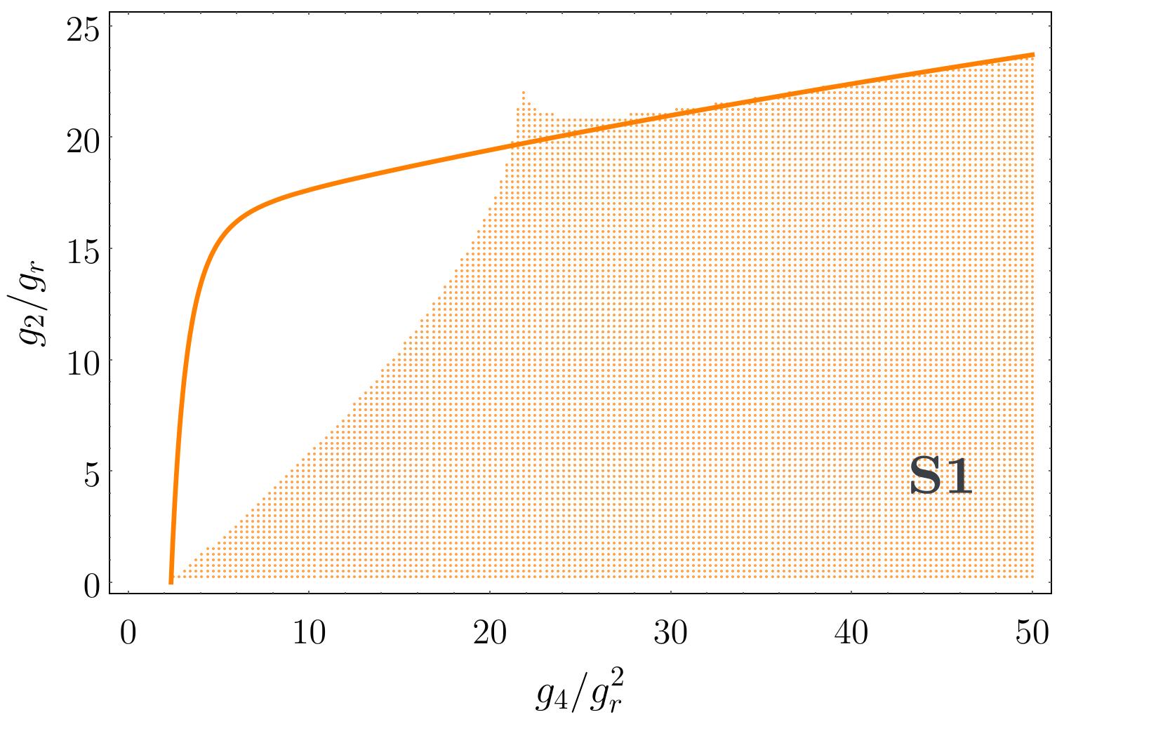
Figure 6: Densely distributed dots indicate the numerically confirmed S1-phase solutions of the $O(g_{r}^{6})$ effective action (4) at ${g_{r}=0.02}$. The solid line represents the corresponding $O(g_{r}^{6})$ analytical S1/S2 transition line (4.35).

We can also determine the support parameters analytically by expanding them in powers of $g_{r}$ and then solving the $z^{0}$ and $z^{-1}$ equations order by order, up to the highest power of $g_{r}$ appearing in the effective action. Once the eigenvalue distribution parameters have been obtained in this way, we turn to the relevant transition condition and solve it in terms of the action couplings. For example, if we wish to express the transition line $g_{2}$ as a function of $g_{4}$, we again expand this function in powers of $g_{r}$ and solve the condition order by order in $g_{r}$. In the case of the S1 to S2 transition, the appropriate condition is the splitting of the eigenvalue distribution support into two parts across the center, i.e.,

$$\rho(g_{i};\,\lambda=0)=0\,,$$ (6.75)

while for S2 to A1 transition, the condition is that the distribution becomes negative at the inner edge of the support, meaning the polynomial part has a zero at that point,

$$H(D-\sqrt{\delta})=0\,.$$ (6.76)

This gives us the transition line equations (4.38) and (4.39). The comparison between the numerical and analytical results mentioned in this section is illustrated in Figure 6 where they display an excellent agreement for larger values of $g_{4}$. However, the analytical expression starts to break down for smaller $g_{4}$ (in this case, near ${g_{4}\approx 25g_{r}^{2}}$), which is a general feature for all the studied orders of approximation.

6.1 Phase Diagram for Second-Order Action

We now apply the methods outlined in the previous section to investigate the simplest multitrace submodel—specifically, the second-order effective action represented by the first line in equation (4), supplemented by the Vandermonde contribution. In this case, the self-consistent integral system simplifies sufficiently to permit an exact solution once the phase transition conditions are imposed.

Notably, in the spirit of (5.69), the eigenvalue distribution equation for the pure potential model with a $\tr^{2}\Phi^{2}$ term is identical in form to that of the standard single-trace quartic model, but with effective couplings shifted by the new term. In particular, one finds modified mass and quartic couplings:

$$g_{2,\text{eff}}=g_{2}-8g_{r}-\frac{64}{3}g_{r}^{2}c_{2}\,,\qquad\qquad g_{4,\text{eff}}=g_{4}-\frac{32}{3}g_{r}^{2}\,.$$ (6.77)

Given the known exact solutions for the S1/S2 and S2/A1 transition lines in the pure potential model, we can use them to derive the corresponding exact transition lines in the presence of the $\tr^{2}\Phi^{2}$ term.

Focusing first on the S1 solution, the exact transition line between the S1 and S2 phases for the second-order effective action was previously obtained in Prekrat:2022sir . It is given by:

$$g_{2}=2\sqrt{g_{4}-\frac{32}{3}g_{r}^{2}}+8g_{r}+\frac{\dfrac{64}{3}g_{r}^{2}}{\sqrt{g_{4}-\dfrac{32}{3}g_{r}^{2}}}\,.$$ (6.78)

We now repeat the used method for the would-be S2/A1 transition line. For the general A1 solution, the support parameters (the $D$ center and the $\sqrt{\delta}$ radius of the support) are obtained by solving the $z^{0}$ and $z^{-1}$ conditions for the resolvent. This yields analytical expressions (as given in Tekel:2015uza ):

$$D=\pm\frac{\sqrt{\displaystyle 3g_{2,\text{eff}}+2\sqrt{g_{2,\text{eff}}^{2}-15g_{4,\text{eff}}}}}{\sqrt{10g_{4,\text{eff}}}}\,,\qquad\quad\delta=2\cdot\frac{g_{2,\text{eff}}-\sqrt{g_{2,\text{eff}}^{2}-15g_{4,\text{eff}}}}{15g_{4,\text{eff}}}\,.$$ (6.79)

Requiring that the arguments of the square roots in (6.79) remain non-negative leads to the following transition line equation:

$$g_{2,\text{eff}}=\sqrt{15\,g_{4,\text{eff}}}\,.$$ (6.80)

Further on, the second moment $c_{2}$ of the A1 eigenvalue distribution satisfying (6.79) can be obtained directly from its definition:

$$c_{2}=\frac{\left(g_{2,\text{eff}}-\sqrt{g_{2,\text{eff}}^{2}-15g_{4,\text{eff}}}\right)\left(41g_{2,\text{eff}}\sqrt{g_{2,\text{eff}}^{2}-15g_{4,\text{eff}}}+49g_{2,\text{eff}}^{2}-120g_{4,\text{eff}}\right)}{1350\,g_{4,\text{eff}}^{2}}\,.$$ (6.81)

Solving the combined equations (6.77), (6.79), (6.80) and (6.81), we obtain the exact would-be transition line between the S2 and A1 phases:

$$g_{2}=\sqrt{15}\sqrt{g_{4}-\frac{32}{3}g_{r}^{2}}+8g_{r}+\frac{\dfrac{1312}{9}g_{r}^{2}}{\sqrt{15}\sqrt{g_{4}-\dfrac{32}{3}g_{r}^{2}}}\,.$$ (6.82)

An inspection of the phase diagram in Figure 7 reveals a region near the $g_{2}$ axis where our system of equations for the eigenvalue distribution lacks solutions. This “void” indicates a domain that is inaccessible within our multitrace model framework. It would be worthwhile to investigate whether HMC simulations applied to the multitrace action yield meaningful configurations in this region.

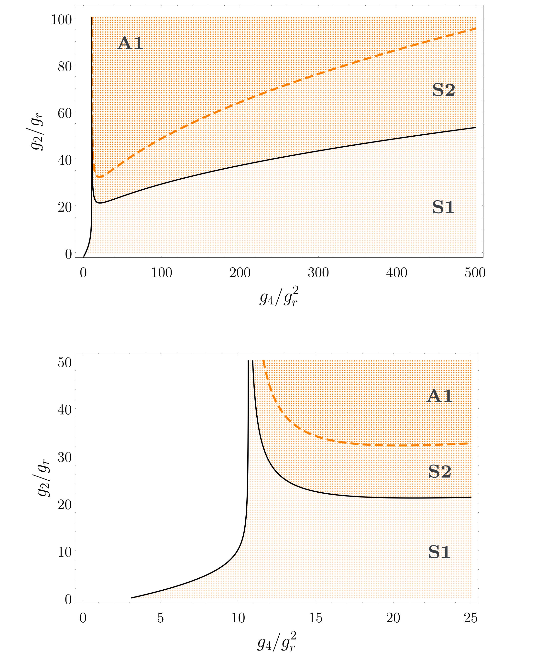
Figure 7: Phase diagram of the second-order action (4) for ${g_{r}=0.02}$, with a zoomed-in view shown in the lower panel. Densely distributed dots in varying shades of orange represent numerically confirmed S1, S2 and would-be A1-phase solutions. The solid black line shows the exact S1-phase boundary, as given by (6.78) and (6.84). The dashed orange line indicates the exact S2/A1 transition line (6.82), which is not realized in this model, as the A1 phase is energetically disfavored compared to the existing S2 phase.

As one moves along the positive $g_{4}$ axis, this void transitions into a region supporting stable S1 solutions for lower values of $g_{2}$. For higher values $g_{2}$ values, the void similarly gives way to an S1 region, which eventually evolves into the S2 phase along the positive $g_{4}$ direction.

The absence of solutions in the void region can be understood by examining the condition for the existence of the S1 solution, specifically, the one arising from the $z^{-1}$-coefficient. For the second-order effective action, this yields the following equation for the support radius $\sqrt{\delta}$:

$$\frac{\delta}{12\left(3-8g_{r}^{2}\delta^{2}\right)}\cdot\left(-18g_{2}+27g_{4}\delta+144g_{r}-288g_{r}^{2}\delta+24g_{4}g_{r}^{2}\delta^{3}-256g_{r}^{4}\delta^{3}\right)=1\,.$$ (6.83)

Solutions to this equation involve several nested square roots. Imposing that the arguments of these roots remain non-negative places constraints on the parameters $g_{r}$, $g_{4}$, and $g_{2}$. The locus where these square roots vanish defines the existence line—the boundary beyond which S1 solutions cease to exist in the phase diagram. For the second-order effective action, this boundary is given explicitly by:

$$g_{2}=-\sqrt{12}\sqrt{-g_{4}+\dfrac{32}{3}g_{r}^{2}}+8g_{r}+\frac{\dfrac{64}{9\sqrt{3}}g_{r}^{2}}{\sqrt{-g_{4}+\dfrac{32}{3}g_{r}^{2}}}\,,\qquad g_{4}<\dfrac{32}{3}g_{r}^{2}\,.$$ (6.84)

Finally, numerical solutions of the aforementioned self-consistent system yield a detailed phase diagram for the second-order effective action (Figure 7), in excellent agreement with the analytically derived exact transition lines and phase boundaries.

7 Monte Carlo Simulation of Full Model

An alternative approach to determining the eigenvalue distributions is to perform Monte Carlo simulations. In particular, we have applied HMC methods betancourt2018conceptual enhanced with an eigenvalue-flipping algorithm Kovacik:2022kfh during the thermalization stage. This combined approach provides nonperturbative insights and is especially valuable for exploring phase transitions in regimes where our analytical approximations break down, i.e. in the $g_{4}\to 0$ limit.

To identify phase transitions from the resulting eigenvalue distributions, we focus on the hallmark of the S1/S2 transition: the splitting of the eigenvalue distribution into two distinct cuts as the system approaches the critical point. In practice, we monitor the midpoint of the eigenvalue distribution moving toward zero as an indicator of this split. Finite-$N$ effects tend to smooth out the emergence of two cuts, so we analyze the distribution behavior over a range of system parameters to pinpoint the transition more reliably. The eigenvalue distributions themselves are obtained from eigenvalue histograms for the field configurations generated by the HMC simulation.

As observed in our previous work Prekrat:2022sir , the midpoint of the eigenvalue distribution decreases approximately linearly with the parameter

$$\gamma=\frac{g_{2}-g_{2}^{*}}{g_{2}^{*}}\,,$$ (7.85)

as the system approaches the transition point $g_{2}^{*}$. In the present study, we extend those findings by incorporating $O(g_{r}^{4})$ contributions to assess the convergence of our numerical results with the analytic prediction. The updated expression for the eigenvalue density at zero (the center of the distribution) is given by

$$\rho(0)=-\frac{\sqrt[4]{4g_{4}}}{\pi}\bigg{(}1+\epsilon-\frac{1}{6}\epsilon^{2} -\frac{1}{2}\epsilon^{3}+\frac{19}{120}\epsilon^{4}\bigg{)}\,\cdot\,$$

$$\,\cdot\,\Bigg{\{}\gamma +\frac{1}{8}\left(1+\epsilon-\frac{8}{3}\epsilon^{2}-3\epsilon^{3}+\frac{16}{5}\epsilon^{4}\right)\gamma^{2}-$$

$$-\frac{1}{6}\epsilon^{2}\left(1+2\epsilon-\frac{7}{3}\epsilon^{2}\right)\gamma^{3}-$$

$$-\frac{1}{512}\left(1+3\epsilon+\frac{49}{3}\epsilon^{2}+40\epsilon^{3}-\frac{722}{5}\epsilon^{4}\right)\gamma^{4}\Bigg{\}}\,.$$ (7.86)

Figure 8 (top panel) illustrates this behavior for ${N=24}$. The “tail” visible in the zoomed-in region of that plot is attributed to finite-$N$ effects. We carried out the procedure of fitting the quadratic function in $\gamma$ (since higher-order terms in (7) are strongly suppressed) to $\rho(0)$ data by incrementally including additional data points. The process was halted once the residuals of the newly added points became significantly larger than typical values and displayed a systematic positive trend—indicating the onset of the tail.

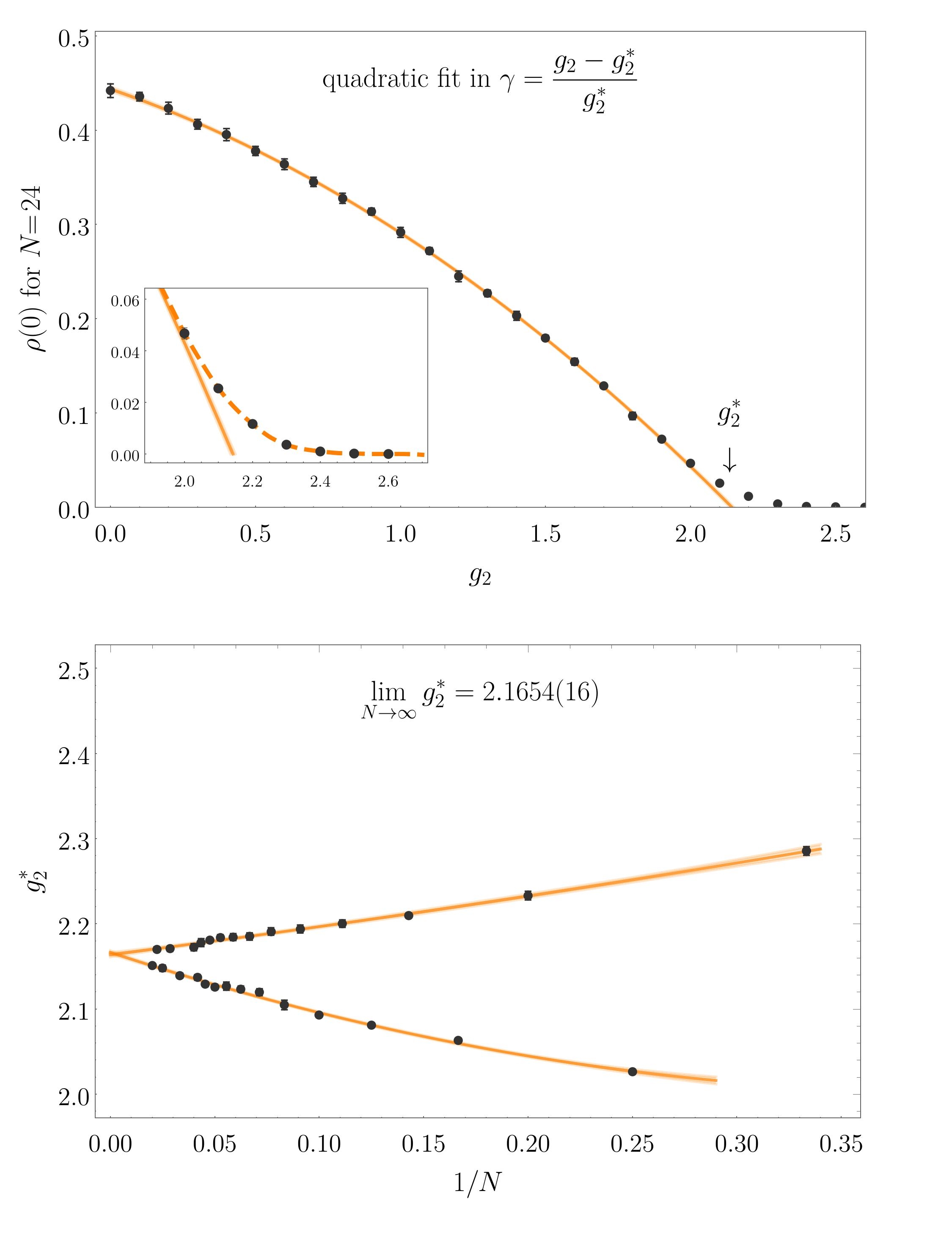
Figure 8: The top panel illustrates how the transition point $g_{2}^{*}$ is extracted from $\rho(0)$ data at fixed $N=24$ (for $(g_{4},\,g_{r})=(1,\,0.02)$) by varying $g_{2}$. The bottom panel shows the extrapolation of the resulting $g_{2}^{*}$ values to the large-$N$ limit. Note that data points for even and odd $N$ fall on separate branches of the curve.

We have then compiled estimates of the transition point $g_{2}^{*}$, the linear coefficient $\#\gamma$

$$\#\gamma\;\leftrightarrow\;\frac{\sqrt[4]{4g_{4}}}{\pi}\left(1+\epsilon-\frac{1}{6}\epsilon^{2}-\frac{1}{2}\epsilon^{3}+\frac{19}{120}\epsilon^{4}\right)\,,$$ (7.87)

and the ratio of the quadratic to linear coefficients $\#\gamma^{2}/\#\gamma$

$$\frac{\,\#\gamma^{2}}{\,\#\gamma^{\phantom{2}}}\;\leftrightarrow\;\frac{1}{8}\left(1+\epsilon-\frac{8}{3}\epsilon^{2}-3\epsilon^{3}+\frac{16}{5}\epsilon^{4}\right)\,,$$ (7.88)

for various values of $N$. To extrapolate these quantities to the ${N\to\infty}$ limit, we performed polynomial fits in $1/N$, using at most quadratic terms. Notably, data points corresponding to even and odd values of $N$ fall on distinct branches in the bottom plot of Figure 8. This bifurcation arises because odd $N$ values exhibit a small local maximum in the eigenvalue density $\rho$ at ${\lambda=0}$, necessitating separate treatment. Our dataset includes matrix sizes up to ${N=50}$. Remarkably, even the use of smaller matrix sizes give consistent albeit less precise $N\to\infty$ results.

To facilitate a comparison between analytical and numerical results, we require error estimates for our analytical predictions. Examining the coefficients in equations (4.39) and (7), we estimate the uncertainties by assuming that the series (7) converge and that the expansion coefficients are of order $O(10^{-1})$ for $g_{2}^{*}$ and $\#\gamma$, and $O(10^{0})$ for $\#\gamma^{2}/\#\gamma$. Truncating the series at order $O(g_{r}^{\tau})$ yields the following error estimates:

$$\Delta g_{2}^{*}\sim 2\sqrt{g_{4}}\sum_{n=\tau}^{\infty}10^{-1}\cdot\epsilon^{n}=\frac{2\sqrt{g_{4}}}{10}\cdot\frac{\epsilon^{\tau}}{1-\epsilon}\,,$$ (7.89)

$$\Delta\#\gamma\sim\frac{\sqrt[4]{4g_{4}}}{\pi}\sum_{n=\tau}^{\infty}10^{-1}\cdot\epsilon^{n}=\frac{\sqrt[4]{4g_{4}}}{10\pi}\cdot\frac{\epsilon^{\tau}}{1-\epsilon}\,,$$ (7.90)

$$\Delta\frac{\,\#\gamma^{2}}{\,\#\gamma^{\phantom{2}}}\sim\frac{1}{8}\sum_{n=\tau}^{\infty}10^{0}\cdot\epsilon^{n}=\frac{1}{8}\cdot\frac{\epsilon^{\tau}}{1-\epsilon}\,.$$ (7.91)

Numerical values corresponding to these error estimates are presented in Tables 1–3, alongside an order-by-order convergence analysis of the transition point. This analysis clarifies the previously observed discrepancy in the $\#\gamma^{2}/\#\gamma$ results reported in Prekrat:2022sir . Specifically, for the value ${g_{r}=0.1}$ used in that study, the convergence of the analytical series was insufficiently rapid, leading to a significant error at the truncation order employed.

$g_{2}^{*}$	$O(g_{r}^{0})$	$O(g_{r}^{2})$	$O(g_{r}^{4})$	$O(g_{r}^{6})$	$\Delta\approx$
$g_{4}=1$, $g_{r}=0.02$	2.000000	2.160000	2.164267	2.164269	$5\cdot 10^{-9}$
$g_{4}=1$, $g_{r}=0.1\phantom{0}$	2.000000	2.800000	2.906667	2.908373	$4\cdot 10^{-3}$

Table 1: Convergence analysis for $g_{2}^{*}$. Each error $\Delta$ corresponds to the estimated uncertainty at the underlined order of approximation, which denotes the highest order reached in the simulation for the specified coupling parameters.

$\#\gamma$	$O(g_{r}^{0})$	$O(g_{r}^{1})$	$O(g_{r}^{2})$	$O(g_{r}^{3})$	$O(g_{r}^{4})$	$\Delta\approx$
$g_{4}=1$, $g_{r}=0.02$	0.45016	0.48617	0.48569	0.48558	0.48558	$2\cdot 10^{-7}$
$g_{4}=1$, $g_{r}=0.1\phantom{0}$	0.45016	0.63022	0.61822	0.60381	0.60564	$5\cdot 10^{-3}$

Table 2: Convergence analysis for $\#\gamma$. Each error $\Delta$ corresponds to the estimated uncertainty at the underlined order of approximation, which denotes the highest order reached in the simulation for the specified coupling parameters.

$\#\gamma^{2}/\#\gamma$	$O(g_{r}^{0})$	$O(g_{r}^{1})$	$O(g_{r}^{2})$	$O(g_{r}^{3})$	$O(g_{r}^{4})$	$\Delta\approx$
$g_{4}=1$, $g_{r}=0.02$	0.12500	0.13500	0.13287	0.13267	0.13269	$5\cdot 10^{-7}$
$g_{4}=1$, $g_{r}=0.1\phantom{0}$	0.12500	0.17500	0.12167	0.09767	0.10791	$2\cdot 10^{-2}$

Table 3: Convergence analysis for $\#\gamma^{2}/\#\gamma$. Each error $\Delta$ corresponds to the estimated uncertainty at the underlined order of approximation, which denotes the highest order reached in the simulation for the specified coupling parameters.

contribution to	$g_{2}^{*}$	$\#\gamma$	$\#\gamma^{2}/\#\gamma$
analytical	0.164269385(5)	0.0354201(2)	0.0076911(5)
numerical	0.1654(16)	0.0348(8)	0.0062(16)

Table 4: Curvature contribution to $g_{2}^{*}$, the linear coefficient $\#\gamma$ and the ratio $\#\gamma^{2}/\#\gamma$ for ${g_{4}=1}$ and ${g_{r}=0.02}$.

We have here obtained high-precision numerical results in a regime where analytical expression (4.39) shows signs of convergence already at order $O(g_{r}^{6})$, specifically:

$$\epsilon\ll 1\quad\Rightarrow\quad g_{4}\gg 16g_{r}^{2}\,.$$ (7.92)

As we can see, the analytical prediction (4.35) aligns exceptionally well with numerical result for the model parameters ${(g_{r},\,g_{4})=(0.02,\,1)}$:

$$\text{analytical:}\qquad g_{2}^{*} \approx 2.164269385(5)\,,$$ (7.93a)

$$\text{numerical:}\qquad g_{2}^{*} \approx 2.1654(16)\,.$$ (7.93b)

Furthermore, the coefficients of $\gamma$ and $\gamma^{2}$ terms closely match the predictions of (7):

$$\text{analytical:}\qquad\rho(0) \approx-0.4855783(2)\cdot\left(\gamma+0.1326911(5)\cdot\gamma^{2}\right)\,,$$ (7.94a)

$$\text{numerical:}\qquad\rho(0) \approx-0.4849(8)\cdot\left(\gamma+0.1312(16)\cdot\gamma^{2}\right)\,.$$ (7.94b)

A more detailed analysis of curvature effects, presented in Table 4, reveals that its contributions to $g_{2}^{*}$ and $\#\gamma$ are confirmed within a 1–2 percent uncertainty. Even the subtler effect in $\#\gamma^{2}/\#\gamma$ is corroborated at approximately the $3.5\sigma$ level.

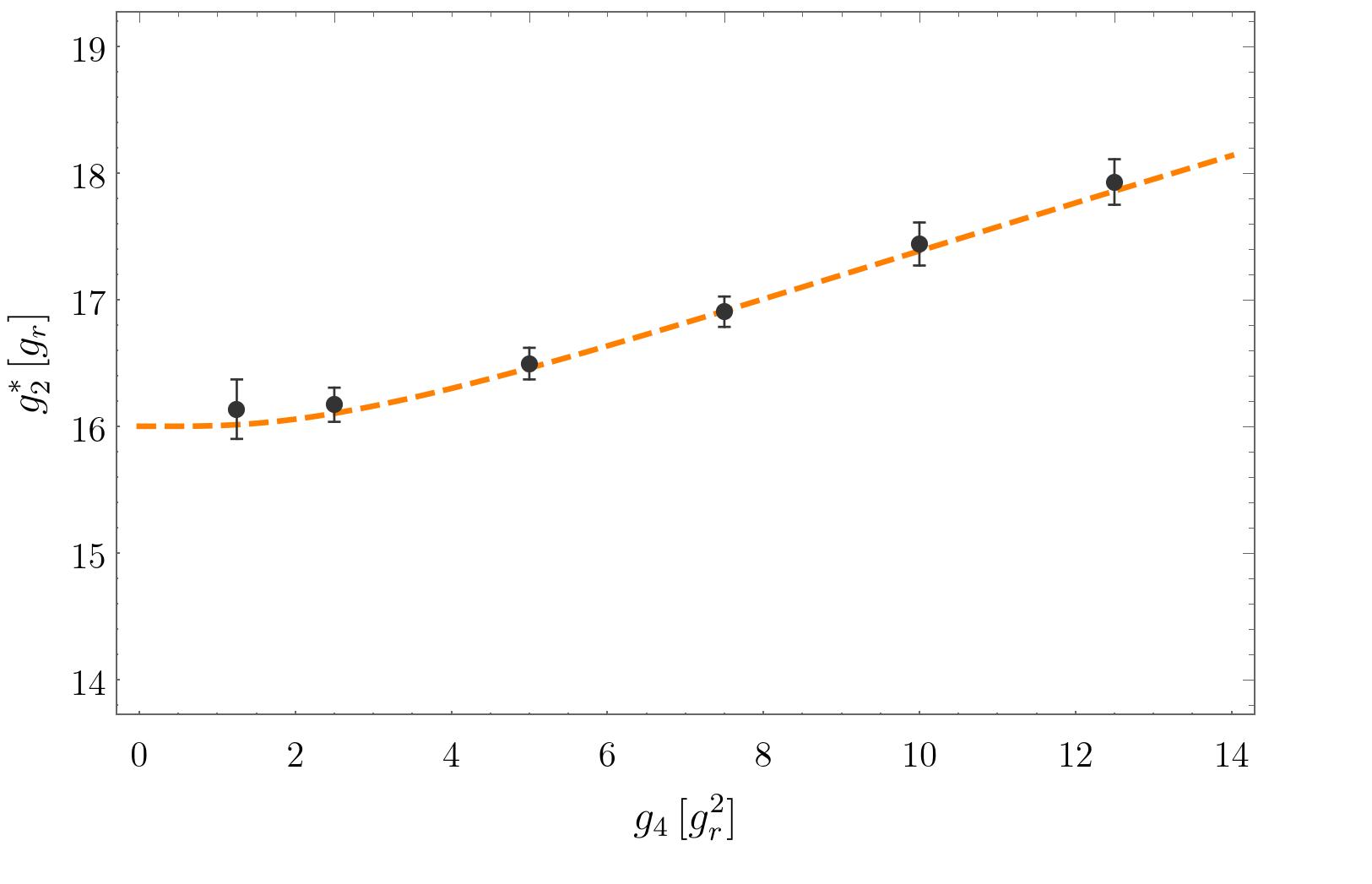
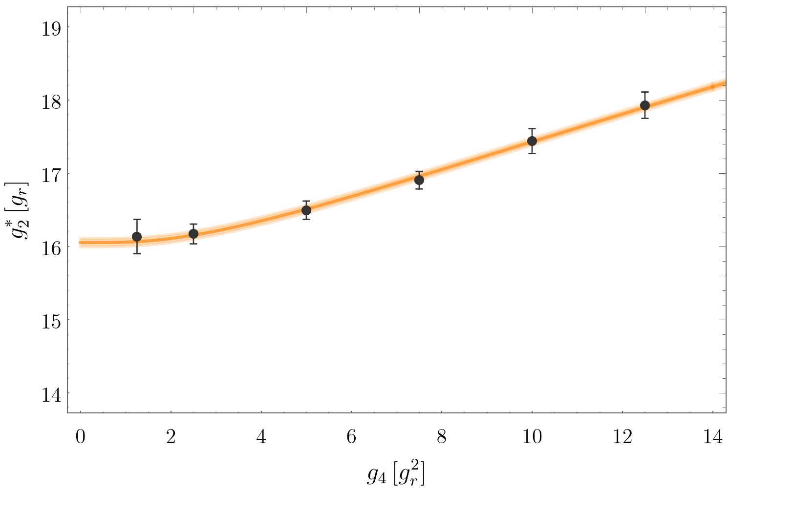
Figure 9: Onset of the S1/S2 transition line for ${g_{r}=0.02}$. The top panel shows the proposed functional form from (7.95). The bottom panel presents a fit of the same form with the coefficient $8g_{r}$ treated as a free parameter. The fit was performed using large-$N$ extrapolated data obtained via HMC simulation of (2.4) without the kinetic term (additional data points lie outside the zoomed-in region). The resulting numerical estimate, ${g_{2}^{*}(0)=16.05(6)g_{r}}$ is in excellent agreement with the expected shift of $16g_{r}$.

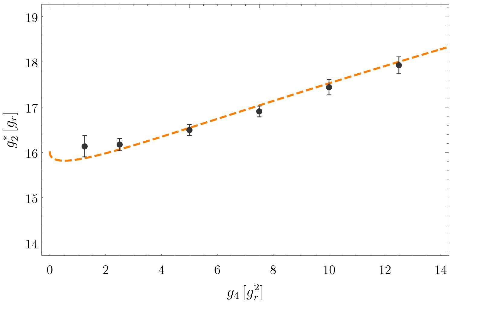
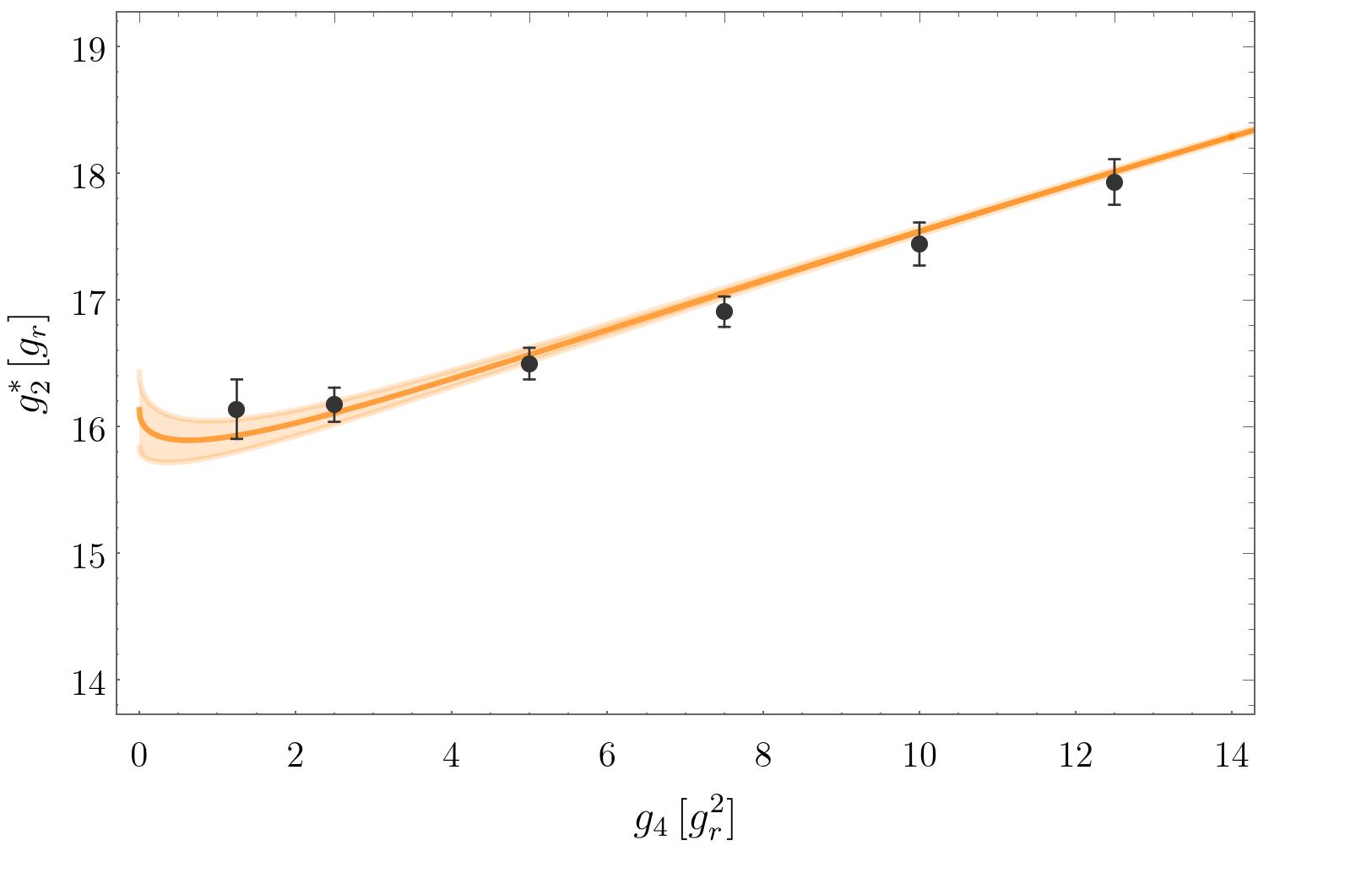
Figure 10: Onset of the S1/S2 transition line for ${g_{r}=0.02}$. The top panel shows the proposed functional form from (7.103). The bottom panel presents a fit of this form with the exponent 3 in (7.102) treated as a free parameter, yielding a fitted value of $3.03(8)$. The fit was performed using large-$N$extrapolated data obtained via HMC simulation of (2.4) without the kinetic term (additional data points lie outside the zoomed-in region). The resulting numerical estimate, ${g_{2}^{*}(0)=16.1(3)g_{r}}$, is consistent with the expected shift of $16g_{r}$.

We have also investigated the regime where ${g_{4}=O(g_{r}^{2})}$, domain in which our perturbative results are no longer reliable. This regime is particularly significant when considering the shift of the triple point. In our previous study Prekrat:2022sir , we proposed the ansatz:

$$g_{2}^{*}=\dfrac{16g_{r}}{1-\exp\left(-\dfrac{8g_{r}}{\sqrt{g_{4}}}\right)}=8g_{r}\left(1+\coth\dfrac{8g_{r}}{2\sqrt{g_{4}}}\right)$$ (7.95)

which shares the same $O(g_{r}^{2})$ expansion as our transition line and provides a good fit to the numerical data. Utilizing this functional form, we performed a non-perturbative fit to our large-$N$ limit data points, as depicted in Figure 9, yielding:

$$g_{2}^{*}=\alpha g_{r}\left(1+\coth\dfrac{\alpha g_{r}}{2\sqrt{g_{4}}}\right),\qquad\alpha=8.03(3)\,.$$ (7.96)

This result implies that the S1/S2 transition line in the $(g_{4},g_{2})$ plane begins at ${g_{4}=0}$ and ${g_{2}=16.05(6)g_{r}}$, consistent with the expected shift of $16g_{r}$ from the origin.

Interestingly, when we express the S1/S2 transition line (4.38) as:

$$\frac{g_{2}-8g_{r}-2\sqrt{g_{4}}}{8g_{r}}=\frac{1}{3}\cdot\epsilon\,+\,\frac{1}{30}\cdot\epsilon^{3}\,-\,\frac{1}{42}\cdot\epsilon^{5}\,,$$ (7.97)

we observe that the coefficients on the right-hand side correspond to differences of Bernoulli numbers:

$$B_{1}-B_{2}=\frac{1}{3}\,,\qquad\quad B_{3}-B_{4}=\frac{1}{30}\,,\qquad\quad B_{5}-B_{6}=-\frac{1}{42}\,.$$ (7.98)

Assuming this pattern continues, and considering the asymptotic expansion of the trigamma function:

$$\psi_{1}(z)\sim\sum_{n=0}^{\infty}\frac{B_{n}}{z^{n+1}}$$ (7.99)

where all odd-indexed Bernoulli numbers (except ${B_{1}=1/2}$) are zero, we propose a new expression for the exact transition line:

$$\frac{g_{2}-8g_{r}-2\sqrt{g_{4}}}{8g_{r}}=\frac{2+\epsilon+\epsilon^{2}}{2\epsilon}-\frac{\psi_{1}\!\left(\epsilon^{-1}\right)}{\epsilon^{2}}\,.$$ (7.100)

As ${g_{4}\to\infty}$ for fixed $g_{r}$, ${\epsilon\to 0}$ and the right-hand side approaches zero, as expected. However, as ${g_{4}\to 0}$, the expression diverges, in stark contrast to our Monte Carlo simulations. The point where the curve turns towards infinity occurs around:

$$g_{4}\approx 0.4\cdot 16g_{r}^{2}<7g_{r}^{2}\,.$$ (7.101)

In our simulations, however, we saw no sign of divergence between the origin and ${g_{4}=7g_{r}^{2}}$ (see Figure 10). This discrepancy suggests that even if the proposed asymptotic series is correct, we need an alternative expression that shares the same series expansion but rectifies the small-$g_{4}$ behavior. This can be achieved by incorporating an exponentially decaying term that lacks an asymptotic series expansion at infinity. For instance, we can implement the desired $16g_{r}$ shift with the following modification (one of many possible choices, but the simplest we found)

$$\frac{\epsilon}{2}\,\,\longrightarrow\,\,\frac{\epsilon}{2}\left(1-\exp\left(-\frac{3}{\epsilon}\right)\right),$$ (7.102)

leading to the revised expression

$$g_{2}=4\sqrt{g_{4}}+12g_{r}+\frac{16g_{r}^{2}}{\sqrt{g_{4}}}\left(1-\exp\left(-\dfrac{3\sqrt{g_{4}}}{4g_{r}}\right)\right)-\frac{g_{4}}{2g_{r}}\cdot\psi_{1}\!\left(\frac{\sqrt{g_{4}}}{4g_{r}}\right),$$ (7.103)

which is plotted in Figure 10.

As shown in Figures 9 and 10, our current data cannot distinguish between the original ansatz (7.95) and the modified expression (7.103) in the ${g_{4}\to 0}$ regime—both appear to describe the simulations equally well within statistical precision. The key difference is that the new expression (7.103) includes a nonperturbative exponential term in $g_{r}$, which was absent in the earlier proposal (7.95).

While examining the model’s behavior at very low $g_{4}$, we encountered a novel feature in the eigenvalue distributions. Instead of the well-known pattern as in Figure 2, the distributions began to exhibit central peaks, with eigenvalues gradually chipping away from the edges of the bulk (see the orange curves in Figure 11). We observed a corresponding signal of this phenomenon in the coefficient ratio $\#\gamma^{2}/\#\gamma$ at low $g_{4}$, where the ratio abruptly starts to decrease from its asymptotic value of $1/8$ toward $0$ (Figure 12). However, we did not observe any accompanying qualitative change in standard thermodynamic observables such as the energy, specific heat, magnetization, susceptibility, or Binder cumulant. Similar effects were noted earlier in Prekrat:2020ptq , and even in the full GW-model with the kinetic term included Prekrat:2023thesis , where a change in susceptibility was seen. However, the matter was not systematically studied and we found indications that the anomaly diminishes as $N$ increases, suggesting that it may be a finite-$N$ artifact rather than a bona fide phase transition.

Figure 11: Eigenvalue distributions in the low-$g_{4}$ regime for ${g_{r}=0.02}$, showing the emergence of central peaks (orange curves) and a gradual depletion of eigenvalues from the edges of the bulk. This deviation from the typical two-cut structure (see Figure 2) may indicate a finite-$N$ artifact or a possible new phase governed by modified vacuum solutions $\Phi_{\!R}$.

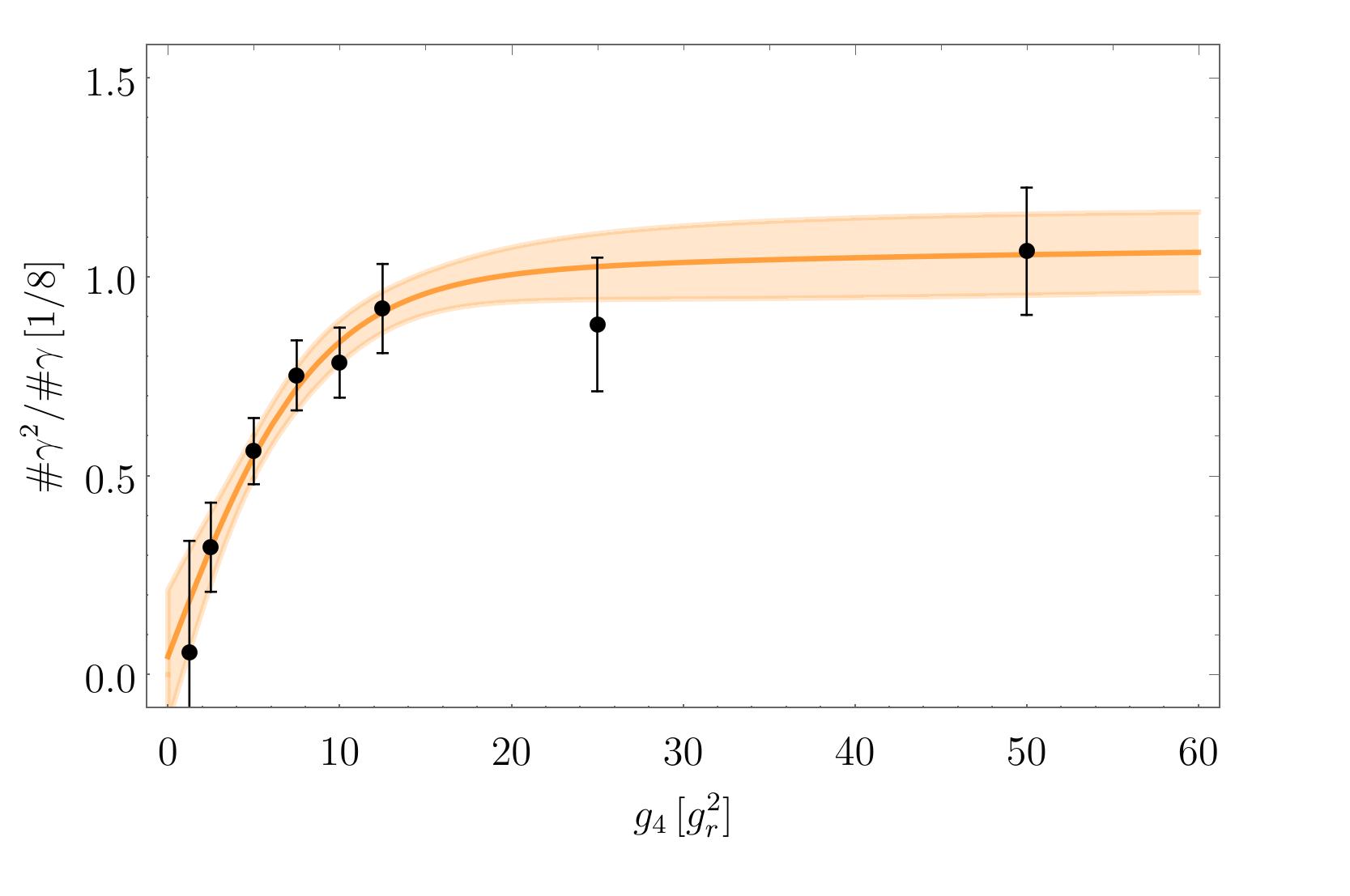
Figure 12: Behavior of the coefficient ratio $\#\gamma^{2}/\#\gamma$ at low $g_{4}$, exhibiting a sharp drop from its asymptotic value of $1/8$ toward zero. This signal correlates with the emergence of central peaks in the eigenvalue distribution (Figure 11), although no corresponding anomaly was observed in thermodynamic observables.

Let us now try to offer explanation for this effect. Consider the exact solution $\Phi_{\!R}$ given by (4.17) which solves the model’s equations of motion in the absence of the kinetic term. This solution is well-defined only for ${g_{2}\geq 16g_{r}}$ so it cannot directly explain what happens for smaller $g_{2}$. However, because the curvature term $R$ is diagonal, we can construct more general solutions by turning off a subset of the eigenvalues. In other words, one can replace some of the eigenvalues in $\Phi_{\!R}$ by zero and still satisfy the equations of motion. The simplest such partially-degenerate solution is

$$(\Psi_{\!R})_{nn}=\begin{cases}(\Phi_{\!R})_{nn}&\text{for }n\leq M\,,\\ 0&\text{for }n>M\,,\end{cases}$$ (7.104)

which is now valid for ${g_{2}\geq 16g_{r}M/N}$.

Let us now examine the Vandermonde (eigenvalue repulsion) contribution to the effective action for the original solution $\Phi_{\!R}$, instead of $\Psi_{\!R}$, for simplicity. This repulsive term is what prevents the eigenvalues from collapsing onto a single value: instead of sharply defined clusters of degenerate eigenvalues (as one might expect from the naive solutions (3.10) with identical eigenvalues), one obtains spread out peaks (as seen in Figure 2). Since there is no eigenvalue degeneracy in $\Phi_{\!R}$, the repulsion is much weaker in this case. Now, assuming $g_{r}$ is small, we can approximate $\Phi_{\!R}$ to first order in $g_{r}$ as

$$\Phi_{\!R}=\sqrt{\frac{g_{2}\operatorname{\mathbb{1}}+g_{r}R}{2g_{4}}}=\sqrt{\frac{g_{2}\mathrlap{\phantom{R}}}{2g_{4}}}\sqrt{\operatorname{\mathbb{1}}+\frac{g_{r}R}{g_{2}}}\approx\sqrt{\frac{g_{2}\mathrlap{\phantom{R}}}{2g_{4}}}\left(\operatorname{\mathbb{1}}+\frac{g_{r}R}{2g_{2}}\right).$$ (7.105)

With this approximation in hand, it is straightforward to show that

$$\Delta(\Phi_{\!R})=\left(-\frac{8g_{r}}{N\sqrt{2g_{2}g_{4}}}\right)^{\!\!\frac{N(N-1)}{2}}\prod_{n=1}^{N-1}n!\,,$$ (7.106)

i.e., the Vandermonde contribution $S_{\Delta}(\Phi_{\!R})\equiv-\ln\Delta^{2}(\Phi_{\!R})$ is

$$S_{\Delta}(\Phi_{\!R}) =-N(N-1)\ln\frac{8g_{r}}{N\sqrt{2g_{2}g_{4}}}-2\ln\prod_{n=1}^{N-1}n!$$ (7.107)

$$\sim N^{2}\ln N-N^{2}\ln\frac{8g_{r}}{\sqrt{2g_{2}g_{4}}}-\left(N^{2}\ln N-\frac{3}{2}N^{2}\right)$$ (7.108)

$$=\left(\frac{3}{2}-\ln\frac{8g_{r}}{\sqrt{2g_{2}g_{4}}}\right)N^{2}\,.$$ (7.109)

On the other hand, the original action (2.4) estimated at $\Phi_{\!R}$ gives

$$S(\Phi_{\!R})=-N\tr\frac{(g_{2}\operatorname{\mathbb{1}}+g_{r}R)^{2}}{4g_{4}}\,,$$ (7.110)

so

$$\frac{S_{\Delta}(\Phi_{\!R})}{S(\Phi_{\!R})}\propto-g_{4}\ln g_{4}\to 0\,,\qquad g_{4}\to 0\,.$$ (7.111)

The $g_{2}$-case is trickier to analyze since $\Psi_{\!R}$-solutions become relevant in the ${g_{2}\to 0}$ limit. Let us first notice that in the ${g_{r}\to 0}$ limit, the Vandermonde contribution to the effective action becomes negligible compared to the classical term. Consequently, we expect the classical solution $\Phi_{\!R}$ to dominate (up to corrections from higher-order terms in $g_{r}$), which is reflected in the sharp eigenvalue peaks seen in the orange curves of Figure 11. Conversely, for larger values of $g_{4}$ the eigenvalues of $\Phi_{\!R}$ move closer together, the Vandermonde repulsion becomes significant, and the resulting distribution more resembles the vacuum solutions in (3.10), as illustrated in the top row of the same figure. Between these two regimes, the sign of the Vandermonde contribution effectively changes, possibly turning eigenvalue repulsion into attraction. This shift could lead to the gradual condensation of eigenvalues near the center, potentially giving rise to the central bulge observed in the orange plots.

8 Conclusions & Outlook

Our results demonstrate that introducing a curvature term into the $\lambda\phi^{4}_{\star}$ model significantly alters its phase structure, most notably by shifting the phase transition lines.

Although we were unable to provide an analytical prediction for the triple point shift via extrapolation from the weak self-coupling regime, we obtained highly precise results in the strong self-coupling limit. These findings were further supported by HMC simulations, which confirmed the expected magnitude of the shift.

This shift plays a pivotal role in the renormalizability of the GW model, as it suppresses the NC stripe phase—known to obstruct renormalization through UV/IR mixing. However, the interplay between this suppression mechanism and the model’s kinetic term remains poorly understood. A complete picture will require disentangling and comparing the respective contributions of the curvature and kinetic terms—an issue currently under investigation.

When viewed in terms of unscaled parameters, the triple point shift effectively removes the stripe phase from the physically relevant region. This applies both to the renormalizable GW model and to the large-$N$ limit of the $\lambda\phi^{4}_{\text{\tiny GW}}$ model, where the curvature coupling vanishes. In contrast, the original, nonrenormalizable $\lambda\phi^{4}$ model lacks such a protective mechanism, with its triple point remaining fixed at the origin of the phase diagram.

Interestingly, we also identified a possible novel phase governed by vacuum solutions modified by the curvature term. Further investigation is required to understand its implications—particularly whether it survives in the large-$N$ limit.

We believe that the link between the absence of the stripe phase and the emergence of renormalizability has broader significance and may extend to other NC models. A natural next step in testing this hypothesis is the simulation of the related—but nonrenormalizable—NC $U(1)$ gauge model Buric:2016lly , which is currently under study. This model features two competing classical vacua: a trivial vacuum and a stripe-like vacuum proportional to the NC coordinates. By identifying which vacuum is energetically preferred, we hope to assess whether the persistence of the stripe phase indeed correlates with nonrenormalizability. Insights of this kind could inform the construction of consistent, renormalizable NC gauge models—an essential step toward generalizing the successes of the GW model beyond scalar field theory.

- (1) S. Hossenfelder, Minimal Length Scale Scenarios for Quantum Gravity, Living Rev. Rel. 16 (2013) 2 [1203.6191].
- (2) H.S. Snyder, Quantized space-time, Phys. Rev. 71 (1947) 38.
- (3) D. Karabali and V.P. Nair, Quantum Hall effect in higher dimensions, Nucl. Phys. B 641 (2002) 533 [hep-th/0203264].
- (4) D. Karabali and V.P. Nair, Quantum Hall effect in higher dimensions, matrix models and fuzzy geometry, J. Phys. A 39 (2006) 12735 [hep-th/0606161].
- (5) S. Donadi and S. Hossenfelder, Toy model for local and deterministic wave-function collapse, Phys. Rev. A 106 (2022) 022212 [2010.01327].
- (6) A.H. Chamseddine, A. Connes and W.D. van Suijlekom, Noncommutativity and physics: a non-technical review, Eur. Phys. J. ST 232 (2023) 3581 [2207.10901].
- (7) C. Blanco and R.K. Leane, Search for Dark Matter Ionization on the Night Side of Jupiter with Cassini, Phys. Rev. Lett. 132 (2024) 261002 [2312.06758].
- (8) M. Door, C.-H. Yeh, M. Heinz, F. Kirk, C. Lyu, T. Miyagi et al., Probing new bosons and nuclear structure with ytterbium isotope shifts, Phys. Rev. Lett. 134 (2025) 063002.
- (9) L. Berezhiani and J. Khoury, Theory of dark matter superfluidity, Phys. Rev. D 92 (2015) 103510 [1507.01019].
- (10) L. Shamir, The distribution of galaxy rotation in jwst advanced deep extragalactic survey, Monthly Notices of the Royal Astronomical Society 538 (2025) 76 [https://academic.oup.com/mnras/article-pdf/538/1/76/61934633/staf292.pdf].
- (11) B. Eynard, T. Kimura and S. Ribault, Random matrices, 10, 2015.
- (12) G. Akemann, J. Baik and P. Di Francesco, The Oxford Handbook of Random Matrix Theory, Oxford Handbooks in Mathematics, Oxford University Press (9, 2011).
- (13) G. Vernizzi, H. Orland and A. Zee, Enumeration of rna structures by matrix models, Phys. Rev. Lett. 94 (2005) 168103.
- (14) C.W.J. Beenakker, Random-matrix theory of Majorana fermions and topological superconductors, Rev. Mod. Phys. 87 (2015) 1037 [1407.2131].
- (15) H.A. Weidenmuller and G.E. Mitchell, Random Matrices and Chaos in Nuclear Physics. Part 1. Nuclear Structure, Rev. Mod. Phys. 81 (2009) 539 [0807.1070].
- (16) T. Guhr, A. Muller-Groeling and H.A. Weidenmuller, Random matrix theories in quantum physics: Common concepts, Phys. Rept. 299 (1998) 189 [cond-mat/9707301].
- (17) R. Loll, Quantum Gravity from Causal Dynamical Triangulations: A Review, Class. Quant. Grav. 37 (2020) 013002 [1905.08669].
- (18) W. Bietenholz, F. Hofheinz, H. Mejía-Díaz and M. Panero, Scalar fields in a non-commutative space, J. Phys. Conf. Ser. 651 (2015) 012003 [1402.4420].
- (19) H. Steinacker, Non-commutative geometry and matrix models, PoS QGQGS2011 (2011) 004 [1109.5521].
- (20) R.J. Szabo, Quantum field theory on noncommutative spaces, Physics Reports 378 (2003) 207.
- (21) J. Rosaler, Dogmas of Effective Field Theory: Scheme Dependence, Fundamental Parameters, and the Many Faces of the Higgs Naturalness Principle, Found. Phys. 52 (2022) 2.
- (22) H. Grosse and R. Wulkenhaar, Renormalization of theory on noncommutative in the matrix base, JHEP 12 (2003) 019 [hep-th/0307017].
- (23) H. Grosse and R. Wulkenhaar, Renormalization of theory on noncommutative R**4 in the matrix base, Commun. Math. Phys. 256 (2005) 305 [hep-th/0401128].
- (24) M. Burić and M. Wohlgenannt, Geometry of the Grosse-Wulkenhaar Model, JHEP 03 (2010) 053 [0902.3408].
- (25) D. Prekrat, Renormalization footprints in the phase diagram of the Grosse-Wulkenhaar model, Phys. Rev. D 104 (2021) 114505 [2104.00657].
- (26) D. Prekrat, D. Ranković, N.K. Todorović-Vasović, S. Kováčik and J. Tekel, Approximate treatment of noncommutative curvature in quartic matrix model, JHEP 01 (2023) 109 [2209.00592].
- (27) S.S. Gubser and S.L. Sondhi, Phase structure of noncommutative scalar field theories, Nucl. Phys. B 605 (2001) 395 [hep-th/0006119].
- (28) J. Tekel, Phase structure of fuzzy field theories and multitrace matrix models, Acta Phys. Slov. 65 (2015) 369 [1512.00689].
- (29) H.Z. Chen and J.L. Karczmarek, Entanglement entropy on a fuzzy sphere with a UV cutoff, JHEP 08 (2018) 154 [1712.09464].
- (30) S. Kováčik and D. O’Connor, Triple Point of a Scalar Field Theory on a Fuzzy Sphere, JHEP 10 (2018) 010 [1805.08111].
- (31) X. Han and S.A. Hartnoll, Deep Quantum Geometry of Matrices, Phys. Rev. X 10 (2020) 011069 [1906.08781].
- (32) S. Kováčik, D. O’Connor and Y. Asano, The nonperturbative phase diagram of the bosonic BMN matrix model, PoS CORFU2019 (2020) 221 [2004.05820].
- (33) B. Ydri and R. Ahmim, Wilsonian renormalization group for a multitrace matrix model, Int. J. Mod. Phys. A 37 (2022) 2250165 [2008.09564].
- (34) B. Ydri, R. Khaled and C. Soudani, Quantized noncommutative geometry from multitrace matrix models, Int. J. Mod. Phys. A 37 (2022) 2250052 [2110.06677].
- (35) D. Prekrat, Phase transitions in matrix models on the truncated Heisenberg space, Ph.D. thesis, University of Belgrade, Faculty of Physics, 03, 2023.
- (36) S. Kováčik and J. Tekel, Fuzzy onionlike space as a matrix model, Phys. Rev. D 109 (2024) 105004 [2309.00576].
- (37) B. Bukor and J. Tekel, Cubic asymmetric multitrace matrix model, 2407.20014.
- (38) M. Šubjaková and J. Tekel, Beyond second-moment approximation in fuzzy-field-theory-like matrix models, JHEP 22 (2020) 065 [2109.03363].
- (39) R. Wulkenhaar, Renormalisation of noncommutative -theory to all orders, Habilitation thesis, TU Wien, Faculty of Physics, 2004.
- (40) P. Castorina and D. Zappala, Spontaneous breaking of translational invariance in non-commutative lambda theory in two dimensions, Phys. Rev. D 77 (2008) 027703 [0711.2659].
- (41) H. Mejía-Díaz, W. Bietenholz and M. Panero, The continuum phase diagram of the 2d non-commutative model, JHEP 10 (2014) 056 [1403.3318].
- (42) J. Ambjorn and S. Catterall, Stripes from (noncommutative) stars, Phys. Lett. B 549 (2002) 253 [hep-lat/0209106].
- (43) B. Ydri, Computational Physics: An Introduction to Monte Carlo Simulations of Matrix Field Theory, World Scientific, Singapore (2017), 10.1142/10283, [1506.02567].
- (44) M. Betancourt, A conceptual introduction to hamiltonian monte carlo, 2018.
- (45) S.F. Viñas and P. Pisani, Worldline approach to the Grosse-Wulkenhaar model, JHEP 11 (2014) 087 [1406.7336].
- (46) D. Prekrat, D. Ranković, N.K. Todorović-Vasović, S. Kováčik and J. Tekel, Phase transitions in a 4 matrix model on a curved noncommutative space, Int. J. Mod. Phys. A 38 (2023) 2343002 [2310.10794].
- (47) M. Šubjaková and J. Tekel, Second moment fuzzy-field-theory-like matrix models, JHEP 06 (2020) 088 [2002.02317].
- (48) B.P. Dolan, D. O’Connor and P. Presnajder, Matrix models on the fuzzy sphere and their continuum limits, JHEP 03 (2002) 013 [hep-th/0109084].
- (49) D. Prekrat, K.N. Todorović-Vasović and D. Ranković, Detecting scaling in phase transitions on the truncated Heisenberg algebra, JHEP 03 (2021) 197 [2002.05704].
- (50) D. Prekrat, D. Rankovic, M. Minic, N.K. Todorovic-Vasovic, S. Kovácik and J. Tekel, (Non)renormalizable noncommutativity in (non)uniform phase, PoS CORFU2023 (2024) 269.
- (51) M. Fukuda, Symbolically integrating tensor networks over various random tensors by the second version of Python RTNI, 2309.01167.
- (52) M. Fukuda, R. König and I. Nechita, RTNI—A symbolic integrator for Haar-random tensor networks, J. Phys. A 52 (2019) 425303 [1902.08539].
- (53) M. Šubjaková and J. Tekel, Fuzzy field theories and related matrix models, PoS CORFU2019 (2020) 189 [2006.12605].
- (54) B. Bukor and J. Tekel, Second order kinetic term effective actions for matrix model description of fuzzy field theories, in Proceedings of the Student Science Conference 2023, FMFI UK, Bratislava, https://zona.fmph.uniba.sk/fileadmin/fmfi/studentska_vedecka_konferencia/zbierka2023/ svk2023_zbornik.pdf.
- (55) S. Kováčik and J. Tekel, Eigenvalue-flipping algorithm for matrix Monte Carlo, JHEP 04 (2022) 149 [2203.05422].
- (56) M. Burić, L. Nenadović and D. Prekrat, One-loop structure of the gauge model on the truncated Heisenberg space, Eur. Phys. J. C 76 (2016) 672 [1610.01429].