The JDISC Survey: Linking the physics and chemistry of inner & outer protoplanetary disk zones

Abstract

Mid-infrared spectroscopy of protoplanetary disks provides a chemical inventory of gas within a few au, where planets are readily detected around older stars. With the JWST Disk Infrared Spectral Chemistry Survey (JDISCS), we explore demographic trends among 31 disks observed with MIRI (MRS) and with previous ALMA millimeter continuum imaging at high angular resolution (5-10 au). With these S/N $\sim$200-450 spectra, we report emission from H₂O, OH, CO, C₂H₂, HCN, CO₂, [Ne II], [Ne III], and [Ar II]. Emission from H₂O, OH and CO is nearly ubiquitous for low-mass stars, and detection rates of all molecules are higher than for similar disks observed with Spitzer-IRS. Slab model fits to the molecular emission lines demonstrate that emission from C₂H₂, HCN, and possibly CO₂ is optically thin; thus since column densities and emitting radii are degenerate, observations are actually sensitive to the total molecular mass. C₂H₂ and HCN emission also typically originate in a hotter region ($920^{+70}_{-130}$, $820^{+70}_{-130}$ K, respectively) than CO₂ ($600^{+200}_{-160}$ K). The HCN to cold H₂O luminosity ratios are generally smaller in smooth disks, consistent with more efficient water delivery via icy pebbles in the absence of large dust substructures. The molecular emission line luminosities are also correlated with mass accretion rates and infrared spectral indices, similar to trends reported from Spitzer-IRS surveys. This work demonstrates the power of combining multi-wavelength observations to explore inner disk chemistry as a function of outer disk and stellar properties, which will continue to grow as the sample of observed Class II systems expands in the coming JWST observation cycles.

1 Introduction

In the classical solar nebula model (e.g., Grossman, 1972), a well-mixed solar-composition gas condenses into solid planetary building blocks, with the local temperature determining which materials condense into the solid phase versus remaining in the gas phase. This results in planets close to the Sun that are more refractory rich, and planets (or planetary cores) that are far from the Sun being more volatile rich. In addition, the condensation of water ice at the Solar System’s so-called “snow line” may have facilitated the formation of more massive planetary cores, seeding the runaway gas accretion needed to form gas giants (e.g., Hayashi, 1981; Pollack et al., 1996; Drażkowska & Alibert, 2017). This classical story is likely incomplete, however, for many reasons. For example, planet-forming regions may inherit minimally processed materials from their parent clouds (e.g. Visser et al., 2011), radial temperature zones are blurred by mixing (e.g. Brownlee et al., 2006), and disk heating may be highly stochastic (e.g. Zhu et al., 2009; Vorobyov & Basu, 2010). The classical story may also require modifications for non-sun-like stars.

Direct measurements of disk chemistry in planet-forming regions are the means to test theories regarding the origin of planetary compositions. This field of study blossomed with the launch of the Spitzer-InfraRed Spectrograph (Houck et al., 2004), from which mid-IR spectra probed disk atmospheres in the terrestrial planet-forming zone (see e.g., Henning & Semenov 2013; Pontoppidan et al. 2014 and references therein). Spitzer-IRS showed that emission from simple molecules, including H₂O, OH, HCN, C₂H₂ and CO₂ was nearly ubiquitous around low-mass stars (Pontoppidan et al., 2010; Carr & Najita, 2011), demonstrating that the study of inner disk chemistry was possible. It was discovered, in contrast, that higher mass Herbig Ae/Be stars only rarely show molecular emission lines, possibly from colder water vapor (Pontoppidan et al., 2010; Fedele et al., 2012). Disks with large inner dust cavities also had minimal molecular emission lines besides CO (Salyk et al., 2009; Pontoppidan et al., 2010; Banzatti et al., 2017), though weaker emission lines, including from photodissociation-produced OH, could be detected with sufficiently high dynamic range (Najita et al., 2010). For full disks around low-mass stars, chemical differences were more difficult to extract, likely due to Spitzer’s relatively low spectral resolution (Salyk et al., 2011b). Nevertheless, intriguing trends in HCN/H₂O line strengths were discovered (Najita et al., 2013, 2018), which later, with larger samples, expanded into trends between water luminosity and the outer disk radius and were potentially linked to inner disk water enrichment by pebble drift (Banzatti et al., 2020).

The James Webb Space Telescope (JWST) Mid InfraRed Instrument Medium Resolution Spectrometer (MIRI-MRS; Rieke et al., 2015; Wells et al., 2015) provides increased sensitivity and spectral resolution compared to Spitzer-IRS, and has already demonstrated a greatly improved ability to tease out chemical details and differences. In particular, MRS has revealed a variety of line strength ratios between H₂O and C-bearing species, including CO₂, HCN and C₂H₂ (e.g. Tabone et al., 2023; Banzatti et al., 2023a; Grant et al., 2023; Xie et al., 2023; Gasman et al., 2023, 2025; Long et al., 2025). It is also possible to “map” molecular emitting regions via modeling of level populations (e.g. Temmink et al., 2024; Romero-Mirza et al., 2024a) and from the observed line broadening (Banzatti et al., 2025; Grant et al., 2024). Evidence for pebble migration followed by water sublimation is now observed in drift-dominated disks (Banzatti et al., 2023a), and trace molecules and isotopologues are detected for the first time (Grant et al., 2023; Perotti et al., 2023; Salyk et al., 2025).

These observations have resulted in the emergence of several new theoretical frameworks. One, which we term “peeling back the onion,” suggests that all disks have an onion-like chemical structure with temperature as the determining factor, but the presence of gaps and rings, known to be nearly ubiquitous from ALMA imaging (Andrews et al., 2018; Long et al., 2018), preferentially reveals different parts of the “onion”. For example, Grant et al. (2023) and Vlasblom et al. (2024) suggest that the stronger CO₂ emission observed in GW Lup relative to water may be caused by an inner disk cavity that is preferentially revealing gas between the H₂O and CO₂ snow lines. A second emerging theoretical idea is that radial pebble drift, or its inhibition, leads to changes in inner disk chemistry. In the inner disk, evidence for pebble drift is arguably strongest in water vapor (Kalyaan et al., 2021; Banzatti et al., 2023a, 2025; Romero-Mirza et al., 2024a; Gasman et al., 2025), but pebble drift is also expected to change the inner disk carbon-to-oxygen elemental ratios and, thus, the ratios of C-bearing to O-bearing molecular abundances (e.g. Najita et al., 2011; Booth et al., 2017; Booth & Ilee, 2019; Mah et al., 2023). A third framework involves the influence of stellar mass on inner disk chemistry (e.g. Pascucci et al., 2009, 2013; Tabone et al., 2023; Xie et al., 2023; Colmenares et al., 2024), with inner disks around lower-mass stars typically, though not always, displaying higher abundances of C-bearing species at ages as old as 30 Myr (Kanwar et al., 2024b; Long et al., 2025). The cause of these differences is still being debated, with leading candidate theories including variations in radial drift rates (Pinilla et al., 2012; Mah et al., 2023), radiation field differences (Walsh et al., 2015), and carbon-grain destruction inside of the so-called soot line (Kress et al., 2010; Tabone et al., 2023; Colmenares et al., 2024). Note that some of these theoretical frameworks predict links between disk dust structure and inner disk chemistry that are potentially observable by combining mid-infrared spectroscopy with dust imaging, especially from the Atacama Large Millimeter/submillimeter Array (ALMA).

To date, many MRS studies of disk chemistry have focused on individual disks, but such studies may not be conducive to revealing global trends related to planet formation chemistry. To more comprehensively characterize the large variety of inner disk molecular spectra observed to date, and to relate this variety to other disk or stellar properties within unified theoretical frameworks, we must begin to analyze larger samples of disk spectra, ideally samples with ancillary disk imaging (see e.g., Banzatti et al. 2023a, 2025; Henning et al. 2024; Gasman et al. 2025). The JWST Disk Infrared Spectral Chemistry Survey (JDISCS; Pontoppidan et al., 2024, and this work) was designed to accelerate this process by building a large sample of MRS observations of protoplanetary disks with high-quality ancillary ALMA imaging. This paper presents a first JDISCS program analysis of all of the disks from our Cycle 1 programs, representing primarily K and M stars of a few Myr age. Section 2 provides an overview of the first sample of JDISCS data from JWST Cycle 1. In Section 3, we describe the basic observables of the sample spectra, including detection statistics of molecular and atomic lines, and retrievals of physical parameters using slab models. Finally, in Sections 4 and 5, we begin to make connections between MRS spectra and dust substructures observed in ALMA data. We conclude with discussions of the next steps needed in this field, notably an expansion towards wider ranges and more complete sampling of the parameter space of star and disk properties.

2 The JWST Disk Infrared Spectral Chemistry Survey (JDISCS)

2.1 Description of the Sample

JDISCS comprises MIRI-MRS data from several GO programs, collectively designed to provide a legacy dataset from which to explore outstanding questions about inner disk chemistry and its link to planet formation. Targets whose outer disks have been well-studied at sub-mm wavelengths are critical to this effort, particularly those that were systematically observed as part of large programs with ALMA. One sample of fundamental importance comes from the ALMA “Disk Substructures at High Angular Resolution Project” (DSHARP; Andrews et al. 2018), which was optimized to search for regions of enhanced sub-mm continuum emission in protoplanetary disks at angular resolutions of $\sim 0.035\arcsec$ (5 au at $d=150$ pc). Such substructures, including rings, gaps, spirals, and azimuthal asymmetries, reveal reservoirs of dust grains that may be trapped in local pressure maxima where they can eventually grow into larger planetesimals (although Dullemond et al. 2018 show that not all substructures are necessarily dust traps). Meanwhile, the chemical conditions of the outer disk have been mapped at the highest sensitivity and spatial resolution to date within a sample of five sources in the “Molecules with ALMA at Planet-Forming Scales” (MAPS; Öberg et al. 2021) survey. The observations provided by these two ALMA programs enable synergic studies between outer disk dust substructures and chemical evolution.

JDISCS adds observations of the chemistry of the terrestrial planet-forming regions to such ALMA data sets. Specifically, the Cycle 1 GO program PID 1584 (PI: C. Salyk; co-PI: K. Pontoppidan) acquired JWST MIRI MRS spectra of 17/20 disks that were included in DSHARP (Andrews et al., 2018). Another three disks are included in the MAPS survey as part of PID 2025 (PI: K. Öberg; Romero-Mirza et al. 2024b). Additional disks are included from PID 1549 (3 disks, PI: K. Pontoppidan; Pontoppidan et al. 2024) and PID 1640 (8 disks, PI: A. Banzatti; Banzatti et al. (2023a); Romero-Mirza et al. (2024a)). These additional disks have moderate-resolution ALMA data ($0.12"$, or 16 au at $d=140$ pc) available from Long et al. (2019a); Hendler et al. (2020) and new unpublished data (Long et al. 2025, in prep). In total, the JDISCS Cycle 1 sample analyzed in this work includes 30 systems (31 disks, since two spectra can be extracted from the binary system AS 205 N + S). Figure 1 presents an overview of the MIRI spectra for different categories of sources observed by JDISCS: the K- and M-type T Tauri stars, the intermediate mass systems, and “transition” disks with large mm cavities. While this first paper includes only Cycle 1 targets, the JDISC Survey now includes targets from Cycles 2 and 3 for a total sample of $\sim$100 disks, including PIDs 3034 (PI: K. Zhang), 3153 (PI: F. Long), and 3228 (PI: I. Cleeves); these additional targets will be analyzed in future works. The JWST data presented in this article were obtained from the Mikulski Archive for Space Telescopes (MAST) at the Space Telescope Science Institute. The specific observations analyzed can be accessed via https://doi.org/10.17909/hx6h-qw97 (catalog doi: 10.17909/hx6h-qw97).

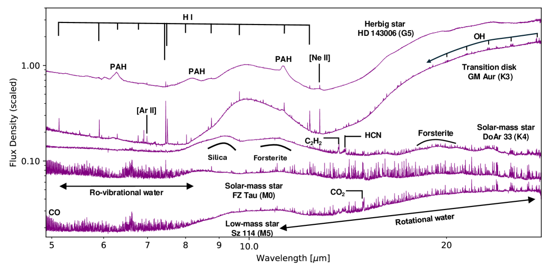
Figure 1: MIRI spectra of select targets from the JDISCS sample, representing broad categories of sources, namely: intermediate mass, transition disk (with a large dust cavity), solar-mass with weak water emission, solar-mass with strong water emission, and a low-mass star. Emission lines from prominent atomic and molecular gas, and solid state features, are highlighted with labels.

Table 2.3 and Table 2.3 list the stellar and outer disk properties for all 31 sources included in this study. Representative spectra for broad categories of sources are highlighted in Figure 1. Figure 2 shows a graphical representation of our coverage of stellar mass, disk radius, and accretion rate. Distances for all targets were obtained by inverting the parallaxes reported in Gaia Data Release 3 (Gaia Collaboration et al., 2016, 2021). Where possible, stellar masses, spectral types, luminosities, mass accretion rates, and sub-mm dust disk masses were taken from the table constructed by Manara et al. (2023), which provides such properties derived from a self-consistent analysis of data from large surveys of star-forming regions (see e.g., Manara et al. 2014, 2016, 2017, 2021; Herczeg & Hillenbrand 2014; Pascucci et al. 2016; Ansdell et al. 2016; Alcalá et al. 2017; Long et al. 2018, 2019a; Testi et al. 2022). This includes stellar masses ($0.16\,M_{\odot}<M_{\ast}<3.58\,M_{\odot}$) and spectral types for all 31 sources (27 K- and M-type T Tauri stars, one G-type star, and three Herbig Ae/Be systems), mass accretion rates for 30/31 $\left(10^{-9.1}\,M_{\odot}\,\rm{yr}^{-1}<\dot{M}_{\rm{acc}}<10^{-6.225}\,M_{\odot}\,\rm{yr}^{-1}\right)$, and sub-mm dust disk masses for 23/31 $\left(2.43\,M_{\oplus}<M_{\rm{dust}}<210.52\,M_{\oplus}\right)$. Stellar properties for the remaining targets were taken from other near- and mid-infrared surveys that are referenced in Table 2.3 (see e.g., Eisner et al. 2005; Salyk et al. 2013; Fairlamb et al. 2015; McClure 2019; Donati et al. 2024). With the sample spanning only a small range in stellar and dust disk masses, the survey is effectively optimized to characterize how the broad diversity of mid-infrared spectra depends on outer disk substructures and mass accretion rates (which span $\sim$4 orders of magnitude; see Figure 2).

We also report the disk inclinations and position angles derived from the sub-mm dust distributions in Table 2.3 (Banzatti et al. 2017; Wu et al. 2017; Huang et al. 2018a, 2020; Kurtovic et al. 2018; Liu et al. 2019; Long et al. 2019b, 2020; Francis & van der Marel 2020; Andrews et al. 2021; Long et al. 2025, in prep). The sample includes inclination angles from $18^{\circ}-67.4^{\circ}$, in addition to one highly inclined target (MY Lup; $i_{\mathrm{disk}}=73.2^{\circ}$). Dust rings are resolved in most disks, while four show spiral arms (AS 205 N, HT Lup A, Elias 27, HD 143006; Kurtovic et al. 2018; Huang et al. 2018b; Andrews et al. 2021) and two have smooth distributions down to $\sim$0.12$\arcsec$, or 16 au (GK Tau, HP Tau; Long et al. 2019b). We note that inner disk substructures at radii that would overlap with the mid-infrared emitting regions are not spatially resolved with ALMA; instead, our dataset can be used to assess the impact of outer disk evolution on inner disk chemistry (see e.g., Najita et al. 2013).

2.2 MIRI-MRS Observations and Data Reduction

The JDISCS data reduction follows that initially described in Pontoppidan et al. (2024). Minor updates since then include reprocessing using the JWST Calibration Pipeline version 1.15.0 and reference file context 1253 (corresponding to the internal JDISCS version 8.0). JDISCS sources observed before 1 January 2024 use the observation of asteroid 526 Jena obtained on 21 September 2023 as part of PID 1549 for MRS channels 2-4, and the observation of early-type star HD 163466 obtained as part of calibration program PID 4499 on 5 July 2023 for channel 1. Extraction aperture radii scale with wavelength as 1.4, 1.3, 1.2, and 1.1 times $1.22\lambda/D$ for MRS channels 1 through 4, respectively. Apertures are kept the same for the source and calibrator, such that any PSF complexities should cancel out during division by the calibrator, improving spectro-photometric precision. Independent observations of HD 163466 suggest that the absolute spectrophotometric precision is a few percent in MRS channels 1-3 and up to 10% at the long wavelength end of channel 4. Future versions of the JDISCS pipeline may achieve higher precision by a combination of multiple calibrators and improved models of the asteroid spectra. The signal-to-noise ratio (S/N) achieved near 17 $\mu$m is 200–450 in all spectra except for HD 163296, which is affected by saturation and fringe residuals.

2.3 Continuum Subtraction

For continuum estimation, we use the automatic iterative algorithm described in Pontoppidan et al. (2024). This method works well in estimating the continuum across all four MIRI channels in conditions of narrow gas emission on top of broad dust emission; however, the continuum level can be uncertain in regions where dense clustering of molecular gas emission lines produce a pseudo-continuum (Carr & Najita, 2011; Pascucci et al., 2013; Tabone et al., 2023; Kanwar et al., 2024b; Arabhavi et al., 2024; Kaeufer et al., 2024a, b). For this reason, we exclude the organic region at 13.4–14.1 $\mu$m from the continuum fit to avoid subtracting part of the emission from HCN and C2H2. In case of strong emission from CO2 (as in MY Lup, HT Lup, Sz 114), we also exclude the 14.9–15 $\mu$m region for the same reason. In case of gas absorption in a wind or a stellar photosphere, an additional adjustment of the continuum is necessary using line-free regions, as described in Banzatti et al. (2025). We discuss the impact of this continuum subtraction method on our analysis and interpretation of the molecular gas emission lines in Section 5.2.

Table 1: JDISCS Stellar Properties

Target	Distance	SpT	$L_{\ast}$	$M_{\ast}$	$\log\dot{M}_{\rm{acc}}$	Radial Velocity
	(pc)		($L_{\odot}$)	($M_{\odot}$)	($M_{\odot}$ yr-1)	(km s-1)
AS 205 N	142	K5	1.3	0.87	-7.4	-5.4
AS 205 S	142	K7+M0	0.7	1.28	$\cdots$	-5.4
AS 209	121	K5	1.4	0.83	-7.3	-9.1
CI Tau	160	K7	0.8	0.65	-7.5	19.9
DoAr 25	138	K5	0.9	0.62	-8.9	-12.6
DoAr 33	142	K4	1.5	0.69	-9.6	-6.6
Elias 20	138	M0	2.6	0.88	-6.7	-3.3
Elias 24	139	K5	6.8	1.10	-6.3	-7.3
Elias 27	110	M0	1.5	0.63	-7.1	-7.7
FZ Tau	129	M0	1.0	0.51	-6.5	15.8
GK Tau	129	K7	0.9	0.58	-8.3	17.0
GM Aur	158	K7	1.0	0.69	-8.0	16.5
GO Tau	140	K5	0.2	0.36	-9.5	17.1
GQ Lup	154	K7	1.4	0.61	-7.4	-2.1
HD 142666	146	A8	9.1	1.23	-8.4	-13.1
HD 143006	167	G7	3.9	1.48	-7.7	-0.2
HD 163296	101	A1	17.0	2.04	-7.4	-4.0
HP Tau	171	K0	1.1	0.84	-10.3	17.7
HT Lup A+B	153	K2	5.1	1.32	-8.1	-1.4
IQ Tau	132	M0.5	1.0	0.42	-7.9	15.3
IRAS 04385+2550	160	M0.5	0.5	0.56	-8.1	17.0
MWC 480	156	A2	22.0	3.58	-7.0	27.7
MY Lup	157	K0	0.9	1.20	-8.0	4.4
RU Lup	158	K7	1.5	0.55	-7.0	-0.8
RY Lup	153	K2	1.9	1.27	-8.1	-0.4
SR 4	135	K7	1.2	0.61	-6.9	-4.5
Sz 114	157	M5	0.2	0.16	-9.1	4.0
Sz 129	160	K7	0.4	0.73	-8.3	3.2
TW Cha	183	K7	0.4	0.70	-8.6	17.8
VZ Cha	191	K7	0.5	0.50	-7.1	16.3
WSB 52	135	M1	1.7	0.55	-7.9	-5.5

Note. — All distances are calculated from Gaia DR3 parallaxes Gaia Collaboration et al. 2023. Stellar properties are taken from the compiled table in Manara et al. 2023, and heliocentric radial velocities are from Banzatti et al. 2019, Fang et al. 2018 and references therein (see below). Significant digits across the sample are rounded to match the targets with the least precise published measurements.

References. — Eisner et al. 2005 (AS 205N, AS 205S); Salyk et al. 2013 (AS 205S, AS 209, CI Tau); Donati et al. 2024 (CI Tau); Gaia Collaboration et al. 2018 (DoAr 25); Cieza et al. 2010 (DoAr 33); Hourihane et al. 2023a (DoAr 33); Testi et al. 2022 (Elias 20, Elias 24, Elias 27, HD 143006, IRAS 04385); Sullivan et al. 2019 (Elias 20, WSB 52); Jönsson et al. 2020 (Elias 24, Elias 27, IRAS 04385, SR 4); McClure 2019 (FZ Tau); Manara et al. 2014 (GM Aur); Alcalá et al. 2017 (GQ Lup, HT Lup A+B, RU Lup, RY Lup); Fairlamb et al. 2015 (HD 142666); Miret-Roig et al. 2022 (HD 142666); Gontcharov 2006 (HD 163296); Kounkel et al. 2019 (IQ Tau); White & Hillenbrand 2004 (IRAS 04385); Najita et al. 2009; Mendigut´ıa et al. 2013 (MWC 480); Alcalá et al. 2019 (MY Lup); Frasca et al. 2017 (MY Lup, Sz 114, Sz 129); Hourihane et al. 2023b (TW Cha); Banzatti et al. 2017 (FZ Tau, TW Cha, VZ Cha); Nguyen et al. 2012 (VZ Cha)

Table 2: Inner and Outer Dust Disk Properties

Target	$n_{13-26}$	$M_{\rm{dust}}$	$r_{\rm{dust}}$	$i_{\rm{disk}}$	PA	Sub-mm	Marker
		($M_{\oplus}$)	(au)	(∘)	(∘)	Substructures
AS 205 N	-0.20	192.9	60	$20$	$114$	spirals	$\mathcal{S}$
AS 205 S	0.50	$\cdots$	34	$66$	$1102$	cavity, ring (34 au)	$\odot$
AS 209	-0.24	$\cdots$	$139$	$35$	$86$	rings (14-141 au)	$\odot$
CI Tau	-0.38	103.4	$174$	$50$	$11$	rings (28-153 au)	$\odot$
DoAr 25	0.23	138.8	$165$	$67$	$111$	rings (86-137 au)	$\odot$
DoAr 33	-1.08	20.3	$27$	$67$	$111$	ring (17 au)	$\odot$
Elias 20	-0.90	54.9	$64$	$49$	$153$	rings (29, 36 au)	$\odot$
Elias 24	-0.83	210.5	$136$	$29$	$46$	rings (77, 123 au)	$\odot$
Elias 27	-0.66	113.8	$254$	$56$	$119$	ring (86 au), spirals	$\mathcal{S}+\odot$
FZ Tau	-1.07	5.3	$\sim$15	$\sim$26	$30$	smooth	$\bullet$
GK Tau	-0.30	2.4	$13$	$40$	$120$	smooth	$\bullet$
GM Aur	2.08	95.9	220	53	57	cavity, rings (40, 84, 168 au)	$\odot$
GO Tau	-0.03	$\cdots$	$144$	$54$	$21$	rings (73, 109 au)	$\odot$
GQ Lup	-0.39	25.6	22	$61$	$346$	gap (10 au)	$\bigcirc$
HD 142666	-0.54	$\cdots$	$59$	$62$	$162$	rings (6-58 au)	$\odot$
HD 143006	1.33	49.7	$82$	$19$	$169$	cavity, rings (6-65 au), spirals	$\mathcal{S}+\odot$
HD 163296	-0.99	$\cdots$	$169$	$47$	$133$	rings (14-155 au)	$\odot$
HP Tau	0.14	27.3	21	$18$	$57$	smooth	$\bullet$
HT Lup A+B	-0.38	49.8	33, 5	$48$	$166$	spirals (A); smooth (B)	$\mathcal{S}$
IQ Tau	-0.63	35.5	$96$	$62$	$42$	rings (48-83 au)	$\odot$
IRAS 04385+2550	0.53	$\cdots$	$\sim 32$	$\sim 60$	$\sim 162$	smooth	$\bullet$
MWC 480	$\cdots$	184.7	$105$	$36$	$148$	ring (98 au)	$\odot$
MY Lup	0.19	50.4	$87$	$73$	$59$	rings (20, 40 au)	$\odot$
RU Lup	-0.14	125.2	$63$	$19$	$121$	rings (17-50 au)	$\odot$
RY Lup	0.45	64.6	80	67	109	cavity (69 au)	$\bigcirc$
SR 4	0.56	38.5	$31$	$22$	$18$	ring (18 au)	$\odot$
Sz 114	-0.16	30.6	$58$	$21$	$165$	ring (45 au)	$\odot$
Sz 129	0.47	58.5	$76$	$34$	$151$	cavity, rings (10-69 au)	$\odot$
TW Cha	-0.03	$\cdots$	$\sim 97$	$\sim 27$	$121$	cavity ($\sim 30$ au)	$\bigcirc$
VZ Cha	-1.22	$\cdots$	$\sim 47$	$\sim 19$	$30$	gap ($<0.1^{\prime\prime}$)	$\odot$
WSB 52	-0.43	36.6	$32$	$54$	$138$	ring (25 au)	$\odot$

References. — Kurtovic et al. 2018 (A205N, AS 205S, HT Lup A+B); Huang et al. 2018a (AS 209, DoAr 25, DoAr 33, Elias 20, Elias 24, Elias 27, HD 142666, HD 163296, MY Lup, RU Lup, SR 4, Sz 114, Sz 129, WSB 52); Long et al. 2019a (CI Tau, GK Tau, HP Tau, IQ Tau); Huang et al. 2020 (GM Aur); Francis & van der Marel 2020 (RY Lup); Long et al. 2020 (GQ Lup; see also Wu et al. 2017); Andrews et al. 2021 (HD 143006); Long et al., private communication (FZ Tau, IRAS 04385+2550, TW Cha, VZ Cha)

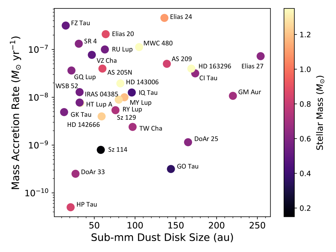
Figure 2: Summary of stellar and disk properties for 30/31 JDISCS targets included in this work, including mass accretion rates (y-axis), sub-mm dust disk radii enclosing 90-95% of the flux at $\sim$1.3 mm (x-axis), and stellar masses (marker colors). The sample spans $\sim$4 orders of magnitude in mass accretion rate, $\sim$2 orders of magnitude in dust disk sizes, and a narrow range in stellar masses (27 K- and M-type T Tauri stars, one G-type star, and three Herbig Ae/Be systems). AS 205 S is excluded from the figure, as it does not yet have a measured accretion rate.

Table 3: Description of JWST MIRI-MRS Observations

Target	Start Date	End Date	Visit ID	Exposure Time
AS 205 N	2023-04-04T16:37:46.419	2023-04-04T17:21:20.598	01584010001	388.504
AS 205 S	2023-04-04T16:37:46.419	2023-04-04T17:21:20.598	01584010001	388.504
AS 209	2022-08-02T02:37:53.904	2022-08-02T04:51:31.158	2025001001	2242.232
CI Tau	2023-02-27T14:03:00.277	2023-02-27T15:56:38.677	1640005001	1776.024
DoAr 25	2023-08-16T04:19:04.241	2023-08-16T05:19:50.954	1584013001	677.108
DoAr 33	2023-03-31T01:26:39.326	2023-03-31T03:15:56.870	1584016001	1687.224
Elias 20	2023-03-31T03:46:55.594	2023-03-31T04:48:07.616	1584012001	721.512
Elias 24	2023-08-16T05:41:51.706	2023-08-16T06:41:15.174	1584014001	654.908
Elias 27	2024-03-16T16:34:36.646	2024-03-16T17:35:15.936	1584021001	677.108
FZ Tau	2023-02-28T03:01:11.403	2023-02-28T04:14:35.498	1549001001	987.916
GK Tau	2023-02-28T04:42:09.445	2023-02-28T05:58:14.500	1640003001	987.916
GM Aur	2023-10-14T11:18:58.286	2023-10-14T14:19:51.433	2025007001	3057.908
GO Tau	2023-10-09T18:51:59.611	2023-10-09T21:14:13.058	1640002001	2319.932
GQ Lup	2023-08-13T14:46:28.511	2023-08-13T16:40:12.236	1640009001	1776.024
HD 142666	2023-04-04T23:57:26.617	2023-04-05T00:40:58.557	1584008001	388.504
HD 143006	2023-04-04T19:35:31.188	2023-04-04T20:35:39.403	1584009001	721.512
HD 163296	2022-08-10T00:42:14.512	2022-08-10T02:56:31.662	2025004001	2253.332
HP Tau	2023-02-27T16:23:53.232	2023-02-27T17:37:00.687	1640001001	987.916
HT Lup A+B	2023-04-04T12:35:49.858	2023-04-04T13:29:51.204	1584001001	588.308
IQ Tau	2023-02-27T11:42:46.236	2023-02-27T13:35:12.413	1640004001	1764.924
IRAS 04385+2550	2023-10-15T22:09:24.933	2023-10-15T23:25:13.620	1640011001	987.916
MWC 480	2023-10-13T07:30:50.504	2023-10-13T09:58:45.508	02025006001	2253.332
MY Lup	2023-08-13T18:58:02.052	2023-08-13T19:50:07.041	1584007001	555.008
RU Lup	2023-08-13T20:11:26.148	2023-08-13T21:02:19.004	1584004001	521.708
RY Lup	2023-08-13T17:10:16.071	2023-08-13T18:24:32.902	1640010001	987.916
SR 4	2023-08-16T02:48:38.943	2023-08-16T03:50:32.240	1584011001	688.208
Sz 114	2023-03-31T12:15:41.650	2023-03-31T13:22:01.166	1584005001	832.512
Sz 129	2023-03-31T07:49:47.701	2023-03-31T09:25:18.832	1584006001	1110.016
TW Cha	2023-07-24T11:32:55.271	2023-07-24T13:57:17.689	1549003001	2386.536
VZ Cha	2023-07-24T14:29:51.363	2023-07-24T16:23:03.536	1549004001	1764.924
WSB 52	2023-08-28T04:47:16.633	2023-08-28T05:30:46.089	1584017001	333.004

3 Results

3.1 Establishing the Inner and Outer Dust Disk Contexts

All JDISCS targets included in this work were observed with ALMA at high angular resolution through DSHARP ($\sim$0.035” or 5 au; Andrews et al. 2018), surveys of the Taurus star-forming region (0.12” or 16 au; Long et al. 2018, 2019a), and a program targeting the remaining disks observed in JWST Cycle 1 that lacked high-resolution mm images (0.05” or 7 au; Long et al., in prep; ALMA Project Code #2021.1.00854.S); we refer the reader to these works for further details about the ALMA observations. While the four programs differ in spatial resolution by a factor of $\sim$4, the closest resolved structures at $\sim$5 au are still outside the expected emitting radii for the mid-infrared molecular gas emission (see e.g., Walsh et al. 2015; Woitke et al. 2018; Anderson et al. 2021; Kanwar et al. 2024a). We use the published sub-mm datasets to provide some outer disk context for the interpretation of inner disk emission lines, with the caveat that we are not able to discern the presence of inner disk dust substructure from the ALMA observations themselves.

As a complementary tracer of inner disk dust evolution, we measure the infrared spectral index $n_{13-26}$ as in Banzatti et al. (2023a) by taking the MIRI continuum flux measured at 13 and 26 $\mu$m. A similar index was previously introduced with Spitzer-IRS spectra at 13 and 30 $\mu$m and was used to infer the presence of an inner dust cavity from positive values of the infrared index $n_{13-30}>0$ (Brown et al., 2007; Furlan et al., 2009; Banzatti et al., 2020). Negative values of $n_{13-30}$ instead indicate emission from abundant small grains in the inner disk region, although inclination effects also play a role (see Appendix D in Banzatti et al., 2020). The specific 13 and 26 $\mu$m wavelength regions used in this work were selected using the analysis in Banzatti et al. (2025) from those that are most free from detectable line emission: at 13.095–13.113 $\mu$m and 26.3–26.4 $\mu$m. At these wavelengths, molecular emission is as weak as the noise on the continuum even in a strong-emission case as CI Tau, which is used for reference in Banzatti et al. (2025). We use 26 $\mu$m instead of 30 $\mu$m due to the different wavelength coverage of the MRS and the S/N that decreases at longer wavelengths. The measured $n_{13-26}$ values for the whole sample are provided in Table 2.3.

Figures 3 and 4 zooms in on the $Q$ branches of C₂H₂, HCN, and CO₂, along with overlapping H₂O transitions, from all JDISCS sources included in this work, ordered by mm dust disk radius from largest (Elias 27; $r\sim 250$ au; Huang et al. 2018a) to smallest (GK Tau; $r\sim 13$ au; Long et al. 2019a). As also observed with Spitzer, the MIRI spectra of the organics are diverse, with clear visual variations in both the shapes and strengths of emission lines across the sample. With the increased spectral resolution of MRS relative to IRS, it is readily apparent where $P$ and $R$ branch transitions of all three molecules overlap, particularly in the case of C₂H₂ and HCN. This makes it challenging to model molecules individually, as the line fluxes at wavelengths corresponding to overlapping transitions can not easily be separated.

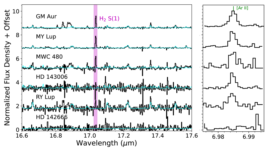
Figure 20: Water emission lines between 16.6-17.6 $\mu$m and [Ar II] emission lines for JDISCS spectra that are dominated by atomic features, with the best-fit H₂O slab models overlaid (cyan). We place upper limits of $\log L_{\rm{emit}}<-5.3,-4.3\,L_{\odot}$ for HD 142666 and HD 143006, respectively. The OH-rich spectrum of GM Aur will be presented in a forthcoming paper (Muñoz-Romero et al., in prep).

The sample presented in Figures 3 and 4 includes five disks with brighter atomic emission lines from H I, [Ne II], [Ne III], and sometimes [Ar II] relative to the molecules: GM Aur, MY Lup, HD 143006, RY Lup, and HD 142666. A set of rotational H₂O emission lines from these systems, where detected, is shown in Figure 20. The group includes one Herbig Ae/Be star (HD 142666), one G-type star (HD 143006), and three T Tauri stars (RY Lup, GM Aur, MY Lup); however, the S/N across the brighter disks (HD 142666, HD 143006, RY Lup) is so high that residual fringing becomes more apparent in the spectra. Since all three targets are brighter than the asteroid calibrators at these wavelengths (along with HD 163296, which is excluded from both Figures 3 and 20 for poor data quality), the JDISCS reduction pipeline cannot yet fully correct for the residual non-linearity in the MIRI detectors. Since this subset of disks is not molecule-rich, the effect does not impact the results presented here.

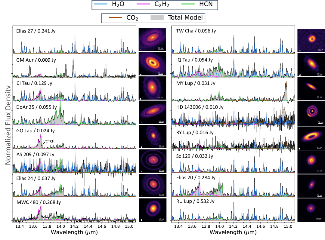
Figure 3: MRS continuum-subtracted spectra of C₂H₂ (magenta), HCN (green), H₂O (blue), and CO₂ (brown) emission lines between 13.6-15.3 $\mu$m from JDISCS sources with sub-mm dust sizes $r>63$ au. ALMA images are shown to the right of the spectra (Andrews et al. 2018; Long et al. 2018, 2019a, Long et al. 2025, in prep), in order of sub-mm dust disk size from largest (top left; Elias 27, $r\sim 250$ au) to smallest (bottom right; RU Lup, $r\sim 63$ au). Slab model fits to the molecular emission lines are overplotted on the spectra, corresponding to the best-fit parameters and upper limits reported in Tables 5, 6, 7, and 10. ¹³C¹²CH₂ emission is also detected in the spectrum of GO Tau, along with multiple CO₂ isotopologues in MY Lup (Salyk et al., 2025), and an OH-rich spectrum with no CO₂ emission from GM Aur (Romero-Mirza et al., submitted).

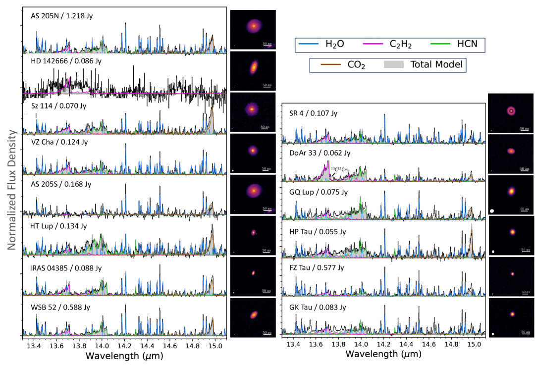
Figure 4: MRS continuum-subtracted spectra of C₂H₂ (magenta), HCN (green), H₂O (blue), and CO₂ (brown) emission lines between 13.6-15.3 $\mu$m from JDISCS sources with sub-mm dust sizes $r<60$ au. ALMA images are shown at right (Andrews et al. 2018; Long et al. 2018, 2019a, Long et al. 2025, in prep), in order of sub-mm dust disk size from largest (top left; AS 205N, $r\sim 60$ au) to smallest (bottom right; GK Tau, $r\sim 13$ au). Slab model fits to the molecular emission lines are overplotted on the spectra, corresponding to the best-fit parameters and upper limits reported in Tables 5, 6, 7, and 10. ¹³C¹²CH₂ emission is also detected in the spectrum of DoAr 33 (Colmenares et al., 2024).

3.2 Detection Rates of H₂O, OH, and CO

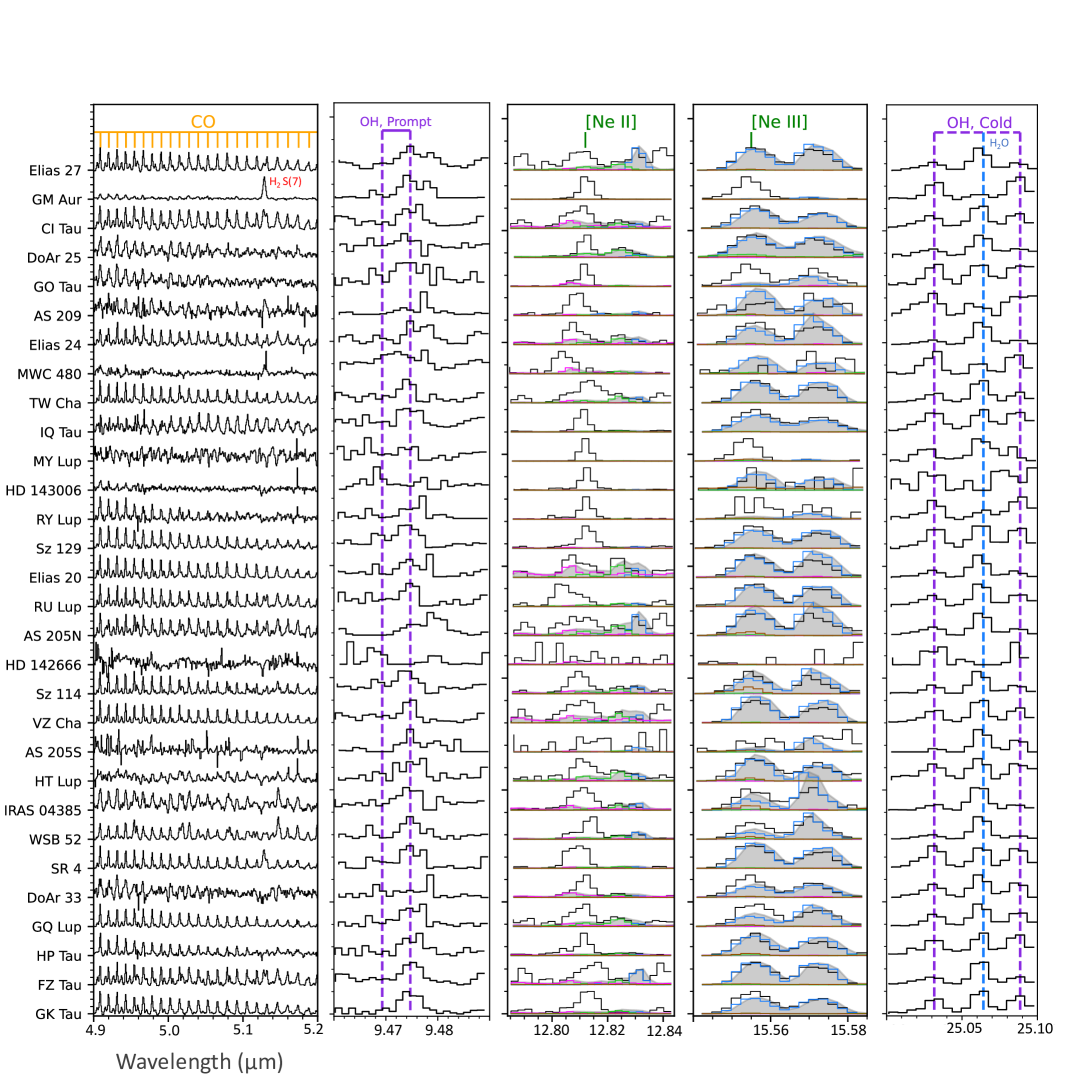
Figure 5: Gallery of ro-vibrational CO, OH, [Ne II], and [Ne III] emission lines from 30/31 JDISCS sources (HD 163296 is excluded due to poor data quality). The spectra are in order from largest to smallest sub-mm disk size, with representative slab models of H₂O overplotted on the data surrounding the [Ne II] and [Ne III] emission lines (following Banzatti et al., 2025). C₂H₂ and HCN slab models are shown as well, with the same color scheme as in Figure 3.

We find that emission lines from H₂O, OH, and CO are nearly ubiquitous at the 2-$\sigma$ threshold across the JDISC sample (see Figures 5 and 11), consistent with previous findings from Spitzer and ground-based spectroscopy surveys (Najita et al., 2003; Pontoppidan et al., 2010; Salyk et al., 2011b; Brown et al., 2013; Banzatti et al., 2022, 2023b). Detailed modeling of these species is required to confirm the fainter lines, but our initial detection rates are reported in Table 4, for the full sample, classical K- and M-type T Tauri stars, transitional disks with infrared spectral indices $>0$, and an “intermediate mass” category that includes all three Herbigs and the G-type star HD 143006. The detection rate for rotational transitions of H₂O is 94%, with HD 142666 and HD 143006 being the only disks where water emission is not detected (Banzatti et al., 2025). Notably, mid-infrared water emission is detected for the first time towards the transition disks RY Lup (Banzatti et al., 2025) and GM Aur (see Figure 20; Romero-Mirza et al. 2025, submitted). While less ubiquitous than the rotational H₂O transitions, ro-vibrational water emission lines are detected in 77% of sources. Non-detections include all three Herbig sources (HD 142666, HD 143006, HD 163296) and the transition disk GM Aur, along with AS 205S, GO Tau, and MY Lup. Ro-vibrational $v=1-0$ CO emission from is observed in 87% of disks with MRS, with the exception of AS 205S, HD 142666, HD 163296 and MY Lup. HD 163296 does have detectable rovibrational CO in ground-based high resolution spectra (Salyk et al., 2011a) as well as water and OH previously detected with Spitzer and Herschel (Fedele et al., 2012).

In the case of OH, we check for detections both in very high energy levels at the short wavelengths and in low energy levels at long wavelengths. We focus on five lines with $E_{u}\sim 27,000-36,000$ K emitting between 9.4 and 10.3 $\mu$m, and six lines with $E_{u}\sim 3000-4000$ K emitting between 23 and 28 $\mu$m. The lines we consider in these ranges are free from water contamination, as determined from the analysis presented in Banzatti et al. (2025). Figure 5 shows examples of these lines near 9.5 $\mu$m and 25 $\mu$m. We detect the high-energy OH lines in 19/30 disks (63% detection rate) and the low-energy lines in 25/30 disks (83% detection rate).

For all of the high-energy OH detections, the lines show the typical asymmetry produced by prompt emission following water photodissociation by UV radiation (e.g. Carr & Najita, 2014; Tabone et al., 2024), suggesting that this may be common in T Tauri disks of a few Myr old. Recent models by Tabone et al. (2024) propose the prompt emission would produce prominent OH lines with a strong asymmetry at $<12$ $\mu$m, but both prominence and asymmetry would become weaker at longer wavelengths due to the increasing separation of transitions and possibly chemical pumping affecting the excitation of OH lines. We note that, contrary to their models, all the OH spectra in our sample show a strong increase in line flux with wavelength, suggesting that either an additional OH reservoir or other excitation processes dominate the observed populations of low-energy lines. We leave a more detailed modeling of water and OH to future work, which will likely require multiple temperature components or a temperature gradient to fully reproduce the emission lines (see e.g., Romero-Mirza et al. 2024a) along with a dedicated treatment of OH emission from disks around intermediate T Tauri stars and Herbig systems.

Table 4: Molecular Detection Rates

Disk Type	N	H2O	OH	CO	CO2	HCN	C2H2
Classical	18	100	94	100	72	94	89
Transitional	9	100	89	78	56	56	56
Intermediate Mass	4	50	50	50	0	0	25
Full Sample	31	94	87	87	58	71	71

3.3 A MIRI-MRS Inventory of Molecular Gas Emission Lines

Figures 3 and 4 highlights the $Q$ branch emission lines from C₂H₂, HCN, and CO₂ from JDISCS targets included in this work. At the exquisite sensitivity and spectral resolution of MIRI across the Channel 3 detector ($R\sim 2190-3160$ between 11.55-17.98 $\mu$m; Pontoppidan et al. 2024), the $P$ and $R$ branch transitions are also now readily detected. These emission lines can remain optically thin even when the lower energy $Q$ branch lines are optically thick, critically breaking the degeneracy between gas temperatures and column densities within the inner disk molecular layer. However, as identified in Spitzer spectra, the emission lines from organic molecules overlap with each other, with rotational H₂O emission lines, and with strong atomic features from H I, [Ne II], and [Ne III]. Even with the increased spectral resolution of MRS, it is challenging to isolate each individual species and characterize temperature and density stratifications within the warm molecular disk surface layers. In fact, previous analyses of MRS spectra have often taken the approach of sequential fits where one molecule is fitted and subtracted before the next molecule is fitted (Grant et al., 2023; Vlasblom et al., 2024), although more recently molecules are fit together (Temmink et al., 2024; Grant et al., 2024).

Instead of measuring line fluxes and reporting detection rates directly from the data, we use local-thermodynamic-equilibrium (LTE) slab models made with spectools-ir (Salyk, 2022) to reproduce the observed spectrum from each disk, measure the total emission line luminosity for each modeled species, and retrieve the underlying physical parameters that describe the molecular gas.

3.3.1 Description of LTE Slab Models

In brief, spectools-ir produces synthetic emission spectra from a slab of gas with three properties: temperature ($T$), column density ($N_{\rm{col}}$), and projected emitting area ($A_{\mathrm{proj}}$), which we convert to an emitting radius ($r_{\rm{slab}}$) assuming A${}_{\mathrm{proj}}=\pi r_{\rm{slab}}^{2}\cos{i_{\mathrm{disk}}}$.

spectools-ir accounts for two fundamental features that are essential for successfully reproducing the observed organic emission lines: line broadening (which is a combination of thermal, instrumental, and Keplerian) and line opacity overlap, which can be particularly significant in the densely clustered spectral regions around the $Q$-branches (Tabone et al., 2023) and for water ortho-para line pairs that overlap in wavelength (Banzatti et al., 2025). In previous work with spectrally unresolved IRS data, the thermal broadening of emission lines was treated as a fixed parameter assumed from the sound speed of H₂ at 1000 K (Salyk et al., 2009). With MRS, emission lines originating from gas populations with different temperatures are now spectrally separated; for example, a warm water emission component ($T\sim 400$ K) has been readily detected against hotter water emission ($T\sim 850$ K) (Banzatti et al., 2023a; Pontoppidan et al., 2024; Romero-Mirza et al., 2024a; Grant et al., 2024; Temmink et al., 2024; Banzatti et al., 2025). These two temperatures correspond to thermal widths (standard deviation) of 0.4 km s^-1 and 0.6 km s^-1, respectively, which differ by a factor of 1.5. This can lead to a significant under- or over-prediction of the model optical depth and a corresponding over- or under-prediction of the column density in order to reproduce the data. Rather than fixing the thermal broadening to a single value across all molecules as assumed in previous IRS analyses and recently in some analyses of MRS spectra (Grant et al., 2023; Tabone et al., 2023; Xie et al., 2023; Banzatti et al., 2023a), we compute it from the temperature used to generate each individual slab model as in Pontoppidan et al. (2024) and Romero-Mirza et al. (2024a). This approach accounts for differences in local line broadening between emission from radially or vertically separated layers of the disk, allowing for better constraints on the column densities retrieved from optically thin features.

At the temperatures and rotation velocities found in inner disks, Keplerian broadening dominates the observed emission line widths as observed at high resolution from the ground (e.g. Najita et al., 2003; Salyk et al., 2011b; Brown et al., 2013; Banzatti et al., 2022). This effect has now been detected also in molecular emission lines observed with MRS, which are broader than the instrument resolution and show, in some disks observed at high inclination, an increase in FWHM as a function of upper level energy (Banzatti et al., 2025). Although the broadening is more challenging to detect in the spectrally unresolved $Q$ branch emission lines from the organic molecules, convolving the water slab models with the instrumental widths alone leads to an under-prediction of emission in the wings of the water line profiles. To account for this, we convolve the slab models to a FWHM measured from the rotational water lines within the same wavelength range as the organics, which represents the contribution from both Keplerian and instrumental broadening (Banzatti et al., 2025).

Further saturation and blending of individual emission lines may be seen when the emitting layer is optically thick (Carr & Najita, 2011; Salyk et al., 2011b; Tabone et al., 2023; Banzatti et al., 2025). spectools-ir accounts for this line opacity overlap by calculating the optical depth as a function of wavelength and summing optical depth over all overlapping transitions before computing flux (see also, Tabone et al. 2023). If this effect is not included, the slab models will consistently over-predict the observed line fluxes and force an under-prediction of the column densities (for the case of water, see Figure 5 in Banzatti et al., 2025). This is particularly important for identifying optically thick populations of gas in the absence of spectrally resolved, optically thin $Q$ branch emission lines (Tabone et al., 2023).

We use slab models generated with spectools-ir to provide fits first to H₂O and subsequently C₂H₂, HCN, and CO₂ emission lines between 12-16 $\mu$m for each disk in our sample. We first use a Markov chain Monte Carlo (MCMC) ensemble sampler (Foreman-Mackey et al., 2013) to fit the water lines, by exploring the temperature, column density, and slab emitting area as variable parameters. The sampler minimizes the L2 loss function, such that

$$\mathcal{L}(\theta)=\sum_{i=1}^{N}\parallel y_{i}-f(x_{i},\theta)\parallel$$ (1)

approaches 0. Here $y_{i}$ represent the observed flux at each wavelength $x_{i}$, and $f(x_{i},\theta)$ is the slab model generated for each $T$, $N_{\rm{col}}$, and $r_{\rm{slab}}$. A statistical analysis that includes the error measurements on the observed fluxes will be included in future works, particularly those searching for emission from isotopologues and rare species, but this simple method sufficiently retrieves best-fit parameters for the more abundant molecules presented here. We also note that the uncertainties produced by degeneracies across the model parameter space far exceed the uncertainties on the flux measurements.

We subtract the best-fit water model from the data to more clearly identify the remaining molecular emission lines and then use a second MCMC ensemble sampler to simultaneously fit all C₂H₂, HCN, and CO₂ emission lines within the same wavelength range. The second sampler also minimizes the L2 loss function; we do not include RMS noise in the loss function, as it is minimal in comparison to the intrinsic model degeneracies. We discuss the impacts of using a single temperature to describe the water emission, excluding fits to low S/N isotopologue emission, and the challenges associated with identifying the true dust continuum in Appendix A and Section 4.

The slab models can also be used to place upper limits on the emitting mass and emission line luminosity from molecules that are not detected in the spectra (see e.g., Salyk et al. 2011b). In other analyses, this has been done molecule-by-molecule (see e.g., Grant et al. 2023; Xie et al. 2023). After subtracting a slab model fit to a single species, the residuals are examined in the wavelength region around the expected $Q$ branch transitions. Marginal and non-detections are identified when an additional molecule does not lead to a significant reduction in the Akaike Information Criterion (Romero-Mirza et al., 2024b), when the RMS noise is equal in strength to the slab model fit (Xie et al., 2023; Schwarz et al., 2024), or when the excess emission is not significant relative to a MRS spectrum in which the molecule is detected (Gasman et al., 2025). While quantitatively robust, iterative fits such as those described in Romero-Mirza et al. (2024b) require significant computational time, making them best suited for carefully characterizing all detected species in a single spectrum and thus prohibitive for this study of 31 sources. For the overview of C₂H₂, HCN, and CO₂ presented here, we set the detection thresholds across the sample by comparing the integrated emission line luminosities from the best-fit slab models and peak-to-continuum ratios calculated as the maximum flux from the same slab models divided by the continuum flux at the corresponding wavelength. We outline this method and discuss its limitations in Section 3.3.3.

3.3.2 Characterizing Rotational H₂O Emission Lines

By fitting transitions between 12–16 $\mu$m only, the slab model fits to water emission lines from 24/31 disks in the JDISCS sample all return similar column densities, with a median value of $\log N_{\mathrm{col}}=18.4$ cm^-2 and standard deviation across the sample of 0.3 dex. This similarity was also identified in the IRS data by Carr & Najita (2011) when the fit was limited to the same spectral range as is done in this work and when all transitions between 10–35 $\mu$m were considered (Salyk et al., 2011b). The median temperature of 710 K derived from the JDISCS sample, with a standard deviation of 100 K, is consistent with those reported in Carr & Najita 2011 for disks around T Tauri stars, which fit over a similar wavelength region. This result is also generally consistent with the hot ($T\sim 800$–900 K) temperature component found in a sub-set of the JDISCS sample in Romero-Mirza et al. (2024a) and Banzatti et al. (2023a), consistent with the fact that higher-energy lines dominate the emission at wavelengths $<$17$\mu$m (Banzatti et al., 2025). Finally, the retrieved emitting areas across the sample correspond to a median slab radius of 0.4 au, with a standard deviation of 0.6 au.

The best-fit H₂O model for each disk was subtracted from the spectrum, leaving water-free residuals which are used to fit the organics and measure atomic emission lines. In Appendix A, we discuss the impact of weak residual water vapor emission on the retrieval of best-fit parameters for the organic molecules. The residual water vapor emission includes signatures of non-LTE excitation in the rovibrational versus rotational states, making them more difficult to reproduce (Meijerink et al., 2009; Bosman et al., 2022; Banzatti et al., 2023a, 2025).

The seven remaining disks (GM Aur, MWC 480, AS 209, HD 142666, HD 143006, MY Lup, and RY Lup) show much stronger residual fringing that overlaps with the water emission lines between 12–16 $\mu$m, making it challenging to identify the best-fit slab model parameters. Instead of fitting this region directly, we fit the slab models to water emission lines between 16.6–17.6 $\mu$m where detected (all these disks except for HD143006, HD142666, MWC 480, and HD 163296) and use those column densities and temperatures to predict a water model at wavelengths that overlap with the organics between 12–16 $\mu$m (see Appendix A, Figure 20). As previously discussed, the disk of HD 163296 is excluded from this analysis due to saturation effects that led to poor data quality.

Appendix A highlights the spectra of two disks around Herbig stars with resolved dust rings (HD 142666 and HD 143006), one disk with a large dust cavity (RY Lup; van der Marel et al. 2018; Francis & van der Marel 2020; Ribas et al. 2024), and one disk with an inner dust gap near $r\sim 8$ au (MY Lup; Huang et al. 2018a) in Figure 20. At the sensitivity of Spitzer-IRS, water emission lines were generally found to be absent in transition disks and were only tentatively detected in some Herbig disks (Pontoppidan et al., 2010), with a firm detection only in HD 163296 (Fedele et al., 2012). A few transition disks (DoAr 44, TW Hya, SR 9), however, did show water emission preferably at longer IR wavelengths (but in the case of DoAr 44 at short IR wavelengths too), indicative of colder water in comparison to what is typically found in T Tauri disks (Salyk et al., 2015; Banzatti et al., 2017). However, we identify water emission lines in the spectrum of RY Lup, with $\log N_{\mathrm{col}}\sim 17.6$ cm^-2 and $T\sim 520$ K. The water emission in MY Lup, instead, can be reproduced with best-fit model indicating $\log N_{\mathrm{col}}\sim 18$ cm^-2 and $T\sim 330$ K (Salyk et al., 2025). The analysis of the sub-sample of disks with dust cavities will be presented in a forthcoming paper (Mallaney et al. 2025 in prep).

3.3.3 A carbon carrier: C₂H₂

We use the IRS and published MRS results to inform the parameter space for slab model retrievals, using uniform priors of C₂H₂ column densities between $10^{13}$ cm${}^{-2}<N_{\mathrm{col}}<10^{24}$ cm^-2, temperatures between 400 K $<T<1500$ K, and slab radii between 0.1 au $<r_{\mathrm{slab}}<3$ au (see e.g., Salyk et al. 2011b; Anderson et al. 2021; Tabone et al. 2023). While cooler, optically thick C₂H₂ emission has been observed in disks around very low mass stars (Tabone et al., 2023), we keep the lower limit on the temperature consistent with what was observed from K- and M-type stars with Spitzer. However, the slab model fits across the 12–16 $\mu$m wavelength range show a strong degeneracy between the column densities and the slab emitting radii. At the same time, the temperatures remain roughly constant with respect to variations in the column densities — see Figure 6. This effect indicates that the emitting gas is optically thin (see e.g., Carr & Najita 2011; Grant et al. 2024), making it challenging to quantitatively converge on a set of best-fit parameters for all disks in the sample without additional prior information.

Within the parameter space identified with IRS observations, we detect clusters of “best-fit” slab model parameters that can reproduce the C₂H₂ emission from each disk, with $<5\%$ changes in the minimum $L2$-norm test statistics. As an example, three possible solutions for AS 205N, shown in Figure 6, are: $\log N_{\mathrm{col}}\sim 15.2$ cm^-2 and $r_{\mathrm{slab}}\sim 2.5$ au, $\log N_{\mathrm{col}}\sim 16.7$ cm^-2 and $r_{\mathrm{slab}}\sim 1.5$ au, and $\log N_{\mathrm{col}}\sim 18.2$ and $r_{\mathrm{slab}}\sim 0.6$ au. This effect was accounted for in analyses of IRS spectra by scaling the slab models to match the observed flux, leaving only the temperatures and column densities as variable parameters in the retrievals (see e.g., Carr & Najita 2008, 2011; Salyk et al. 2011b).

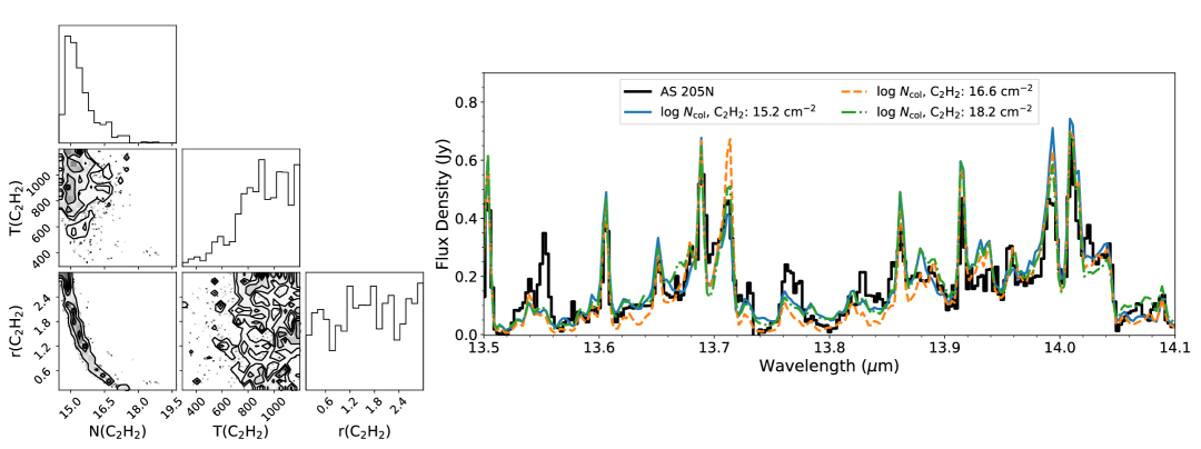
Figure 6: Left: Example corner plot, showing the strong degeneracy between column density and slab radius in LTE slab model fits to the C₂H₂ emission from AS 205N. The effect is still apparent when HCN and CO₂ emission lines are included in the fit. Right: Degenerate slab model solutions overlaid on JDISCS spectrum of AS 205N.

Additional solutions appear when the parameter space is extended to include smaller or larger slab radii (see also, Carr & Najita 2011). Anderson et al. (2021) find that CO₂ and C₂H₂ emission can come from radii as large as 3–5 au, making all degenerate slab model fits consistent with the physical-chemical models presented in that work. However, the low $\log N_{\mathrm{col}}$ solutions are close to the column densities used to place upper limits on the C₂H₂ emission from IRS ($N_{\mathrm{col}}\sim 10^{13}-10^{14}$ cm^-2; Carr & Najita 2011; Salyk et al. 2011b). The slab emitting areas were treated as scale factors in that work, requiring smaller values to reproduce the non-detections than the large slab radii that are consistent with the detected emission lines in the JDISCS spectra. Meanwhile, the optically thick $N_{\mathrm{col}}>10^{18}$ cm^-2 solutions should have resulted in ubiquitous detections of the ¹³C¹²CH₂ isotopologue assuming ¹²C/¹³C $\approx 70$ (Tabone et al., 2023; Kanwar et al., 2024b; Arabhavi et al., 2024), which is only unambiguously detected in two JDISCS sources (DoAr 33 and GO Tau; Colmenares et al. 2024).

For all other disks where the molecules are detected but the isotopologues are not, we plot the slab models generated from the intermediate solutions. An example retrieved model is shown for AS 205N in Figure 7, which has bright emission lines from H₂O, C₂H₂, HCN, and CO₂. Rather than interpreting the slab model parameters themselves, we carry out our analysis using the total number of molecules (measured from the column density and emitting area to eliminate the degeneracy, and converted to units of $M_{\oplus}$), gas temperatures, and integrated model luminosities, as all three quantities are generally better preserved across the degenerate solutions. This means that model fits with identical $L2$-norm test statistics have temperatures, emitting masses, and luminosities that are similar to each other, even when the retrieved column densities and slab radii are not.

The computation time to achieve true convergence of the MCMC chains for the full sample is prohibitively expensive at this time (see e.g., Romero-Mirza et al. 2024b; Grant et al. 2024); instead, we measure (or retrieve) each metric from the set of all unique slab models with $L2$-norm test statistic values within 5% of the best-fit solution (consistent to within roughly 2$\sigma$; see Equation 1). We report the median values and standard deviations in Table 5.

We set a rough detection threshold for each of the three organic molecules considered in this work based on the integrated emission line luminosities measured from the best-fit slab models (see Figure 8). For C₂H₂, the $Q$ branch is readily identified when the integrated emission line luminosity between 12-16 $\mu$m exceeds $\log(L/L_{\odot})\sim-5.1$. With this metric, C₂H₂ is detected in 22/31 sources, for a detection rate of 71%. This is a significant increase over the 43-44% detection rate reported for K and M type T Tauri stars observed with IRS (Pontoppidan et al., 2010; Carr & Najita, 2011); we note that our sample includes five of the disks with previous IRS detections (AS 205, DoAr 25, IQ Tau, TW Cha, VZ Cha). The disks with C₂H₂ detections in JDISCS have a median slab temperature of $920^{+70}_{-130}$ K — see all retrieved temperatures in Figure 9. The coolest temperatures are reported for SR 4 and DoAr 33 ($T\sim 700$ K; see also, Colmenares et al. 2024), and five disks have temperatures $>1000$ K. The group of sources with the highest C₂H₂ temperatures includes the four disks with the smallest sub-mm dust radii in our sample: GK Tau ($r_{\mathrm{dust}}=13$ au), FZ Tau ($r_{\mathrm{dust}}=15$ au), HP Tau ($r_{\mathrm{dust}}=21$ au), and GQ Lup ($r_{\mathrm{dust}}=22$ au). The final disk, Sz 129, has a larger sub-mm dust disk ($r_{\mathrm{dust}}=76$ au) and the smallest inner disk C₂H₂ mass of the sample ($M=5.8\times 10^{-10}\,M_{\oplus}$). We compare these results to the HCN and CO₂ slab model parameters in the following sections.

3.3.4 A nitrogen carrier: HCN

HCN is one of three expected nitrogen carriers within inner disk gas (including NH₃ and N₂; Pontoppidan et al. 2019), and it is as yet the only one that is readily detected in both IRS and ground-based mid-infrared spectroscopy (see Najita et al. 2021 for a TEXES detection of NH₃ in absorption, Kaeufer et al. 2024b for a tentative detection of NH₃ with MRS). HCN emission is detected at a similar rate to C₂H₂ in our sample, with integrated emission line luminosities from the best-fit slab models exceeding $\log(L)\sim-5.1\,L_{\odot}$ in 22/31 sources (71%). Of the nine sources from which HCN was not observed, four are disks around Herbigs or intermediate mass T Tauri stars and four are transitional disks with $n_{13-26}>0$. The exception is AS 209 (see Romero-Mirza et al. 2024b for discussion of a marginal detection). This result is roughly consistent with the 60–70% detection rate of HCN emission lines reported in analyses of solar-mass IRS spectra (Pascucci et al., 2009; Pontoppidan et al., 2010; Carr & Najita, 2011).

Figure 9 shows that the HCN slab temperatures are generally consistent with the C₂H₂ temperatures across the sample, with a median temperature of $820^{+70}_{-130}$ K. The integrated emission line luminosities and emitting masses of the two molecules are also generally similar (see Figure 10). The hottest temperature in the sample is retrieved from DoAr 25 ($T=950\pm 70$ K); however, the total HCN mass from this target falls near the median total HCN mass of the JDISCS sample ($1.4\times 10^{-8}\,M_{\oplus}$, compared to the sample median of $1.2\times 10^{-8}\,M_{\oplus}$), so it does not appear to be unusually HCN-rich. Although HCN is readily detected, we do not detect the HC₃N $Q$ branch that is identified in other sources with MIRI (Kanwar et al., 2024b; Kaeufer et al., 2024b; Arabhavi et al., 2024; Long et al., 2025), prominent emission from NH₃ (Kaeufer et al., 2024b), or H¹³CN (Salyk et al., 2025).

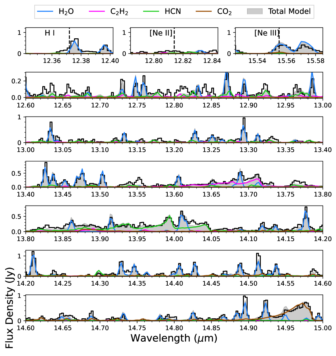
Figure 7: MIRI-MRS spectrum of the brightest disk between 12-16 $\mu$m in our sample, AS 205N (black), with slab model fits to emission lines from H₂O (blue), C₂H₂ (magenta), HCN (green), and CO₂ (brown), as an example of a JDISCS target with prominent emission lines from all four molecules. The total model is shaded in gray. The complete set of similar figures for all targets in our sample is available in the online journal and https://github.com/narulanantham/JDISCS_Cyc1_slabmodelfits.git.

3.3.5 An oxygen carrier: CO₂

Like H₂O, CO₂ is a primary carrier of oxygen in the inner disk. MRS observations have revealed reservoirs of warm CO₂ that are abundant enough for robust detection of the ¹³CO₂ isotopologue $Q$ branch near 15.4 $\mu$m (Grant et al., 2023). MY Lup is the only JDISCS source in which the CO₂ isotopologues are unambiguously detected (Salyk et al., 2025), although Sz 114 has a marginal detection of ¹³CO₂ (Xie et al., 2023). The detection threshold of ¹²CO₂ from our slab model fits to the JDISCS sample is more ambiguous than the minimum peak-to-continuum ratios at which C₂H₂ and HCN are observed see Figure 8), due to overlap with H I (16-10) emission at 14.962 $\mu$m that appears similar in shape to the CO₂ $Q$ branch (see e.g., GM Aur; Romero-Mirza et al., submitted). We identify 14/31 disks with integrated CO₂ emission line luminosities larger than $\log(L)\sim-5.1\,L_{\odot}$. An additional four disks show CO₂ $Q$ branches upon visual inspection of the data, for a total detection rate of 18/31 (58%). Since these targets have emission line luminosities and peak-to-continuum ratios that are similar to those disks in which CO₂ emission is not detected, any criterion that includes them will capture the non-detections as well.

The ¹²CO₂ spectra in the JDISCS sample display the largest diversity in slab model parameters of all four molecules considered in this work, with best-fit temperatures ranging from 330–1050 K. AS 205N and MY Lup have the largest CO₂ masses in our sample ($3.7\times 10^{-7}\,M_{\oplus}$), while IQ Tau has the smallest ($2.3\times 10^{-10}\,M_{\oplus}$). The median temperature of $600^{+200}_{-160}$ K is significantly cooler than the median C₂H₂ and HCN temperatures of $920^{+70}_{-130}$ K and $820^{+70}_{-130}$ K, respectively. We note that this is likely an upper limit on the median CO₂ temperature, as the CO₂ slab models are slightly over-predicted in the $P$ and $R$ branch emission lines. Since the peak-to-continuum ratios in the $Q$ branches are similar to the overlapping H₂O emission lines, in addition to the aforementioned H I transition, CO₂ may be particularly dependent on the number of temperature components used to model the H₂O. We also find that the CO₂ emission line luminosities are slightly weaker than those from C₂H₂ and HCN and the emitting masses slightly higher (see Figure 10). These effects are discussed further in Section 4.1.

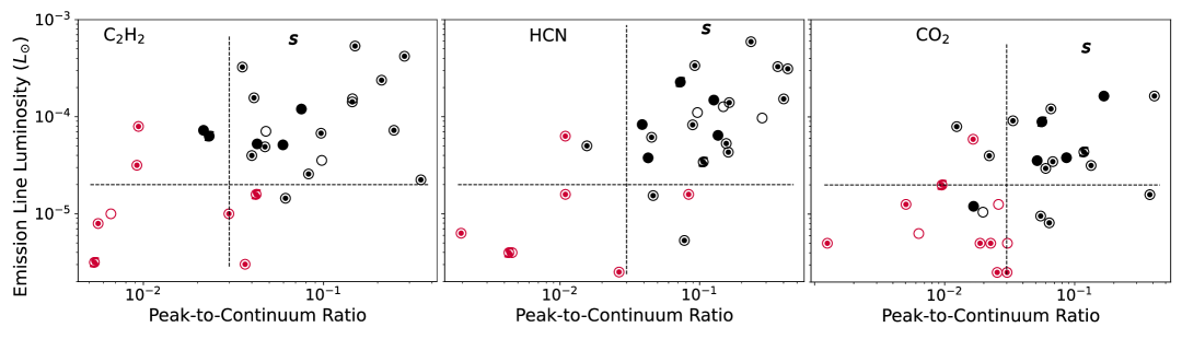
Figure 8: Emission line luminosities from best-fit slab models (integrated between 12-16 $\mu$m) versus peak-to-continuum values from the slab models and fit to the continuum, with marker styles indicating the spatially resolved sub-mm structures in Table 2.3. Targets in the upper right quadrant show the clearest molecular gas detections, and we report non-detections (red markers) when peak-to-continuum ratios are $<0.03$ or emission line luminosities are smaller than $\log L<-5.1\,L_{\odot}$ (black, dashed lines). While disks with resolved sub-mm dust cavities show C₂H₂ and HCN emission lines, none of these sources have CO₂ emission.

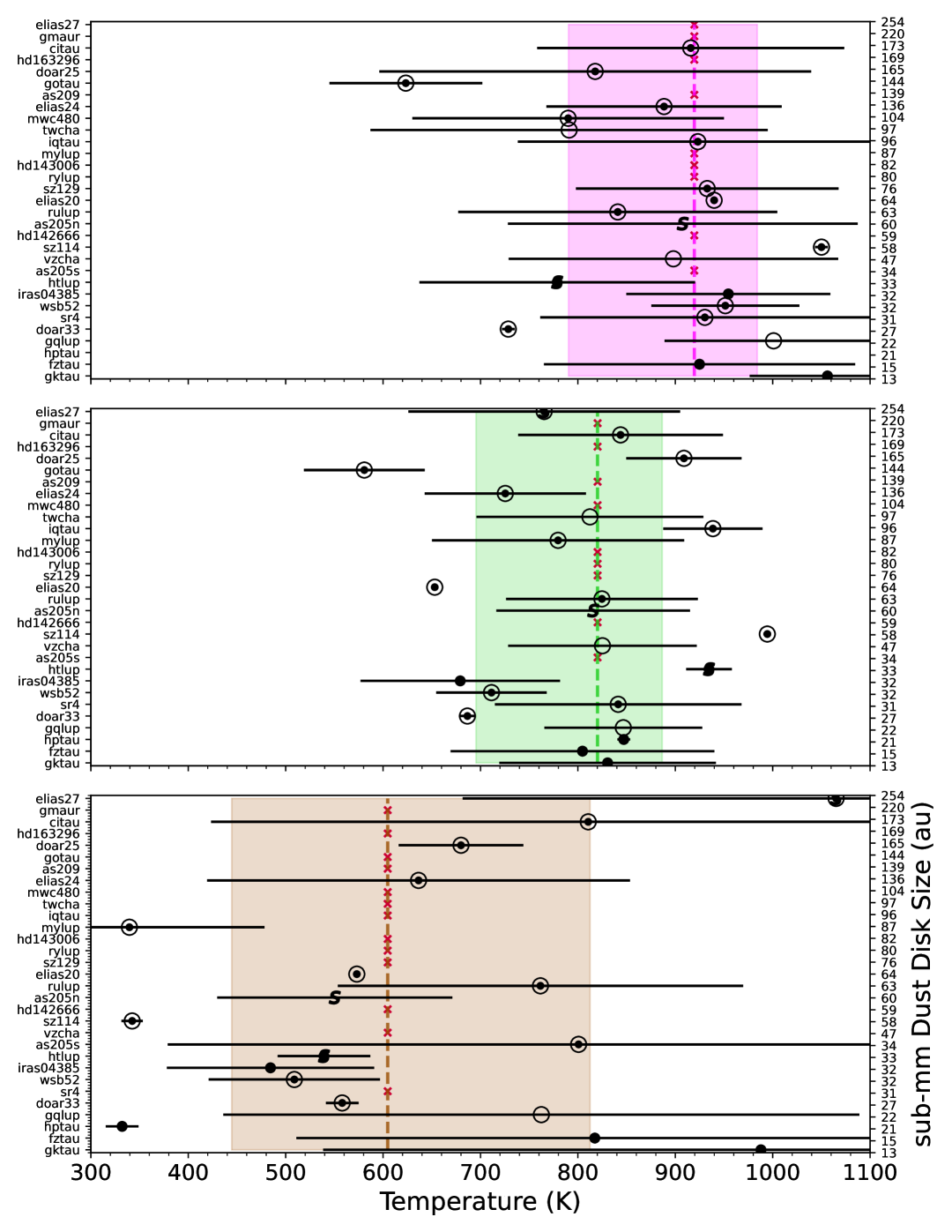
Figure 9: Retrieved temperatures from slab model fits to C₂H₂ (top, magenta), HCN (middle, green), and CO₂ (bottom, brown) emission lines from JDISCS sources in order of decreasing sub-mm disk size from top to bottom of each panel. Vertical dashed lines and shaded regions represent the sample median $\pm 1\sigma$, with red x’s along the median lines denoting non-detections for each molecule. Black markers identify the sub-mm substructures, as listed in Table 2.3. The C₂H₂ and HCN temperatures are generally consistent, while the CO₂ is cooler.

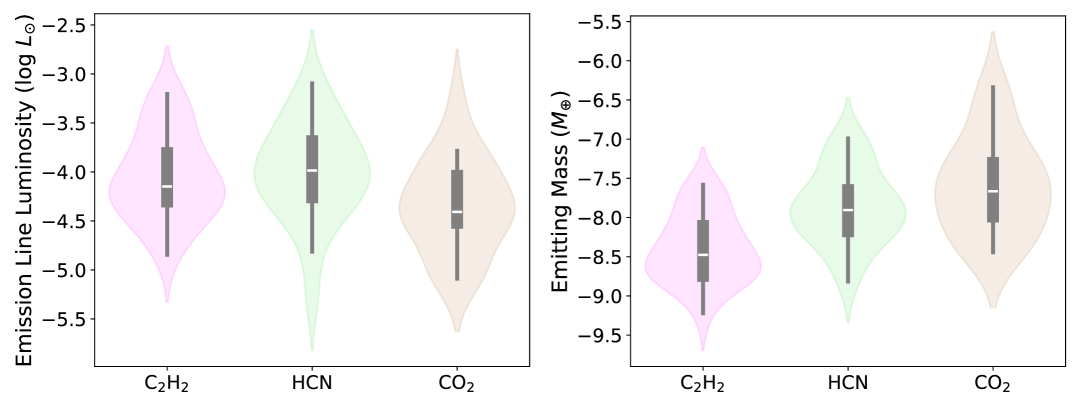
Figure 10: Emission line luminosities (left) and emitting masses (right) integrated from slab model fits to C₂H₂, HCN, and CO₂ between 12-16 $\mu$m in JDISCS sources. Despite spanning a limited range in stellar masses, the targets display at least an order of magnitude variation in mid-infrared luminosity and mass of each molecule. Violin widths represent the number of disks with detections of each molecule, such that narrower violins correspond to lower detection rates.

Table 5: Slab Model Fit Parameters: C₂H₂

Target	$\log N$	$r_{\text{slab}}$	$M_{\text{emit}}$	$T$	$L_{\text{emit}}$	P/C
	(cm-2)	(au)	$\log M$ ($M_{\oplus}$)	(K)	$\log L$ ($L_{\odot}$)
AS 205 N	16.5	0.4	-7.6	$910\pm 180$	-3.2	0.068
AS 205 S	$\cdots$	$\cdots$	$<-9.3$	$\cdots$	$<-5.1$	$<0.006$
AS 209	$\cdots$	$\cdots$	$<-8.7$	$\cdots$	$<-4.5$	$<0.009$
CI Tau	15.6	0.6	-8.2	$920\pm 160$	-3.8	0.144
DoAr 25	14.6	0.8	$-8.9$	$820\pm 220$	$-4.59$	$0.083$
DoAr 33	15.0	0.9	-8.4	$730\pm 10$	-4.1	0.246
Elias 20	15.4	1.1	-7.8	$940\pm 100$	-3.4	0.282
Elias 24	15.8	0.9	-7.6	$890\pm 120$	-3.3	0.150
Elias 27	$\cdots$	$\cdots$	$<-9.2$	$\cdots$	$<-4.8$	$<0.042$
FZ Tau	15.2	0.9	-8.3	$920\pm 160$	-3.9	0.075
GK Tau	15.0	0.6	-8.7	$1060\pm 80$	-4.3	0.043
GM Aur	$\cdots$	$\cdots$	$<-9.6$	$\cdots$	$<-5.52$	$<0.037$
GO Tau	15.2	0.5	-8.8	$620\pm 80$	-4.65	0.347
GQ Lup	14.9	0.7	-8.6	$1000\pm 100$	-4.2	0.048
HD 142666	$\cdots$	$\cdots$	$<-8.4$	$\cdots$	$<-4.1$	$<0.009$
HD 143006	$\cdots$	$\cdots$	$<-9.2$	$\cdots$	$<-5.5$	$<0.005$
HD 163296	$\cdots$	$\cdots$	$\cdots$	$\cdots$	$\cdots$	$\cdots$
HP Tau	14.2	1.8	-8.6	$1130\pm 100$	-4.1	0.022
HT Lup	15.7	0.3	-8.4	$780\pm 140$	-4.2	0.023
IQ Tau	14.8	0.7	-8.8	$920\pm 180$	-4.4	0.060
IRAS 04385	14.5	1.4	-8.7	$950\pm 100$	-4.3	0.040
MWC 480	16.0	0.7	-7.8	$790\pm 160$	-3.5	0.04
MY Lup	$\cdots$	$\cdots$	$<-9.3$	$\cdots$	$<-5.0$	$<0.030$
RU Lup	15.3	0.7	$-8.1$	$840\pm 160$	-3.8	0.041
RY Lup	$\cdots$	$\cdots$	$<-9.4$	$\cdots$	$<-5.0$	$<0.007$
SR 4	15.1	0.6	-8.5	$930\pm 170$	-4.2	0.047
Sz 114	14.5	1.1	-8.8	$1050\pm 100$	-4.3	0.097
Sz 129	14.4	0.7	$-9.2$	$930\pm 130$	$<-4.8$	$<0.062$
TW Cha	14.9	0.7	-8.8	$790\pm 200$	-4.5	0.098
VZ Cha	15.8	0.4	-8.2	$900\pm 170$	-3.8	0.145
WSB 52	15.1	1.1	-8.0	$950\pm 100$	-3.6	0.210

Note. — Since $\log N$ and $r_{\rm{slab}}$ are degenerate, we do not include them in the analysis (see Section 3.3.3). The values reported here are those used to generate the slab models shown in Figures 3 and 4. We use the set of slab model solutions within $<5\%$ of the minimum $L2$-norm test statistic for each disk to derive the median total number of molecules ($M_{\rm{emit}}$) and integrated emission line luminosities between 12-16 $\mu$m ($L_{\rm{emit}}$).

Table 6: Slab Model Fit Parameters: HCN

Target	$\log N$	$r_{\text{slab}}$	$M_{\text{emit}}$	$T$	$L_{\text{emit}}$	P/C
	(cm-2)	(au)	$\log M$ ($M_{\oplus}$)	(K)	$\log L$ ($L_{\odot}$)
AS 205 N	16.9	0.6	-7.0	$820\pm 100$	-3.1	0.112
AS 205 S	$\cdots$	$\cdots$	$<-8.6$	$\cdots$	$<-4.8$	$<0.03$
AS 209	$\cdots$	$\cdots$	$<-8.1$	$\cdots$	$<-4.3$	$<0.01$
CI Tau	15.7	0.7	-7.8	$840\pm 110$	-3.9	0.163
DoAr 25	17.0	0.2	-7.8	$910\pm 100$	-3.8	0.401
DoAr 33	14.8	1.4	-8.1	$690\pm 100$	-4.4	0.161
Elias 20	15.3	2.3	-7.2	$650\pm 100$	-3.5	0.363
Elias 24	15.3	2.6	-7.1	$730\pm 100$	-3.2	0.233
Elias 27	15.3	0.6	-8.3	$770\pm 140$	-4.5	0.106
FZ Tau	15.0	2.3	-7.7	$800\pm 140$	-3.8	0.127
GK Tau	14.3	2.6	-8.3	$830\pm 110$	-4.4	0.043
GM Aur	$\cdots$	$\cdots$	$<-9.4$	$\cdots$	$<-5.6$	$<0.03$
GO Tau	15.0	0.6	-8.8	$580\pm 100$	-5.3	0.078
GQ Lup	15.1	1.3	-7.9	$850\pm 100$	-4.0	0.097
HD 142666	$\cdots$	$\cdots$	$<-9.0$	$\cdots$	$<-5.2$	$<0.002$
HD 143006	$\cdots$	$\cdots$	$<-9.2$	$\cdots$	$<-5.4$	$<0.004$
HD 163296	$\cdots$	$\cdots$	$\cdots$	$\cdots$	$\cdots$	$\cdots$
HP Tau	14.7	1.9	-8.0	$850\pm 100$	-4.1	0.039
HT Lup	16.6	0.4	-7.7	$930\pm 100$	-3.6	0.073
IQ Tau	15.1	1.1	-8.1	$940\pm 100$	-4.1	0.136
IRAS 04385	14.6	2.7	-7.9	$680\pm 100$	-4.2	0.089
MWC 480	$\cdots$	$\cdots$	$<-8.0$	$\cdots$	$<-4.2$	$<0.01$
MY Lup	14.9	0.9	-8.7	$780\pm 130$	-4.8	0.046
RU Lup	15.1	2.5	-7.4	$820\pm 100$	-3.5	0.092
RY Lup	$\cdots$	$\cdots$	$<-9.2$	$\cdots$	$<-5.4$	$<0.005$
SR 4	15.0	1.1	-8.2	$840\pm 130$	-4.3	0.045
Sz 114	14.1	2.9	-8.3	$990\pm 100$	-4.2	0.155
Sz 129	$\cdots$	$\cdots$	$<-8.7$	$\cdots$	$<-4.8$	$<0.08$
TW Cha	15.1	1.5	-7.9	$810\pm 120$	-4.0	0.281
VZ Cha	17.5	0.2	-7.8	$830\pm 100$	-3.9	0.148
WSB 52	16.1	0.8	-7.3	$710\pm 100$	-3.5	0.429

Note. — Since $\log N$ and $r_{\rm{slab}}$ are degenerate, we do not include them in the analysis (see Section 3.3.3). The values reported here are those used to generate the slab models shown in Figures 3 and 4. We use the set of slab model solutions within $<5\%$ of the minimum $L2$-norm test statistic for each disk to derive the median total number of molecules ($M_{\rm{emit}}$) and integrated emission line luminosities between 12-16 $\mu$m ($L_{\rm{emit}}$).

Table 7: Slab Model Fit Parameters: CO₂

Target	$\log N$	$r_{\text{slab}}$	$M_{\text{emit}}$	$T$	$L_{\text{emit}}$	P/C
	(cm-2)	(au)	$\log M$ ($M_{\oplus}$)	(K)	$\log L$ ($L_{\odot}$)
AS 205 N	16.5	1.1	-6.5	$550\pm 120$	-3.3	0.122
AS 205 S	14.9	1.8	-7.8	$800\pm 420$	-4.4	0.022
AS 209	$\cdots$	$\cdots$	$<-7.9$	$\cdots$	$<-4.1$	$<0.01$
CI Tau	15.1	1.1	-8.0	$810\pm 390$	-4.5	0.060
DoAr 25	14.2	1.7	-8.4	$680\pm 100$	-5.0	0.055
DoAr 33	14.8	0.9	-8.3	$560\pm 100$	-5.1	0.064
Elias 20	14.9	1.6	-7.7	$570\pm 100$	-4.5	0.068
Elias 24	16.0	0.6	-7.3	$640\pm 220$	-3.9	0.066
Elias 27	15.7	0.6	-8.0	$1070\pm 380$	-4.4	0.118
FZ Tau	14.7	2.8	-7.3	$820\pm 310$	-3.8	0.168
GK Tau	14.3	2.5	-8.4	$990\pm 450$	-4.9	0.017
GM Aur	$\cdots$	$\cdots$	$<-9.0$	$\cdots$	$<-5.6$	$<0.03$
GO Tau	$\cdots$	$\cdots$	$<-9.1$	$\cdots$	$<-5.6$	$<0.03$
GQ Lup	15.6	0.6	-8.3	$760\pm 330$	-5.0	0.020
HD 142666	$\cdots$	$\cdots$	$<-8.8$	$\cdots$	$<-5.3$	$<0.001$
HD 143006	$\cdots$	$\cdots$	$<-8.4$	$\cdots$	$<-4.7$	$<0.01$
HD 163296	$\cdots$	$\cdots$	$\cdots$	$\cdots$	$\cdots$	$\cdots$
HP Tau	15.7	1.3	-7.1	$330\pm 100$	-4.5	0.051
HT Lup	16.6	0.5	-7.4	$540\pm 100$	-4.1	0.056
IQ Tau	$\cdots$	$\cdots$	$<-8.7$	$\cdots$	$<-5.3$	$<0.02$
IRAS 04385	16.1	0.5	-7.6	$480\pm 110$	-4.4	0.086
MWC 480	$\cdots$	$\cdots$	$<-8.3$	$\cdots$	$<-4.9$	$<0.005$
MY Lup	19.9	0.2	-7.8	$340\pm 140$	-4.5	0.134
RU Lup	16.5	0.3	-7.5	$760\pm 210$	-4.0	0.034
RY Lup	$\cdots$	$\cdots$	$<-8.8$	$\cdots$	$<-5.2$	$<0.006$
SR 4	$\cdots$	$\cdots$	$<-8.3$	$\cdots$	$<-4.8$	$<0.02$
Sz 114	17.3	0.5	-6.3	$340\pm 100$	-4.2	0.378
Sz 129	$\cdots$	$\cdots$	$<-9.0$	$\cdots$	$<-5.3$	$<0.02$
TW Cha	$\cdots$	$\cdots$	$<-8.7$	$\cdots$	$<-5.3$	$<0.03$
VZ Cha	$\cdots$	$\cdots$	$<-8.4$	$\cdots$	$<-4.9$	$<0.03$
WSB 52	15.5	2.4	-6.8	$510\pm 100$	-3.8	0.410

Note. — Since $\log N$ and $r_{\rm{slab}}$ are degenerate, we do not include them in the analysis (see Section 3.3.3). The values reported here are those used to generate the slab models shown in Figures 3 and and 4. We use the set of slab model solutions within $<5\%$ of the minimum $L2$-norm test statistic for each disk to derive the median total number of molecules ($M_{\rm{emit}}$) and integrated emission line luminosities between 12-16 $\mu$m ($L_{\rm{emit}}$).

3.4 A Comparison of Molecule Detection Rates from Spitzer and JWST

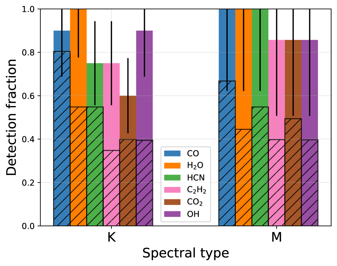
Figure 11: Detection rates of CO, H₂O, HCN, C₂H₂, CO₂ and OH for K and M stars in this sample of MRS spectra. Hatches show IRS or ground-based (for CO) detection rates from Pontoppidan et al. (2010). Earlier spectral types are excluded from this plot due to low number statistics in the JDISCS sample.

Figure 11 compares the detection rates of H₂O, OH, C₂H₂, HCN, and CO₂ in K and M stars from this work to the Spitzer-IRS sample from Pontoppidan et al. (2010). The detection rates with MIRI-MRS are significantly higher for all five molecules; however, we note that there are only eight targets in this paper that were also included in Pontoppidan et al. (2010) and Salyk et al. (2011b). The disks with new detections that we report here, which were non-detections with Spitzer, are HT Lup (H₂O, HCN, C₂H₂), DoAr 25 (H₂O, CO₂), RY Lup (H₂O), and RU Lup (C₂H₂).

DoAr 25 and RY Lup both have positive infrared spectral indices ($n_{13-31}>0$), which classified them as transition disks in the Spitzer era. While transition disks were expected to be molecule-poor, the detections in both sources indicate that MIRI-MRS is sensitive to smaller line-to-continuum ratios than the IRS (see also, Perotti et al. 2023). The remaining disks have detections and non-detections that are consistent between JWST and Spitzer; notably, CO₂ emission is still not detected in RY Lup, TW Cha, or VZ Cha. The overall factor of two increase in CO₂ detection rates may be attributed to the improvement in spectral resolution and signal-to-noise ratios provided by the MRS. Since fewer disks in Figure 8 have CO₂ peak-to-continuum ratios $>0.1$ than C₂H₂ or HCN peak-to-continuum ratios $>0.1$, the CO₂ $Q$ branch lines that are now readily detected were likely too weak to resolve with Spitzer.

3.5 An Inventory of Atomic Jet, Wind, and Accretion Tracers

Figure 5 shows a gallery of [Ne II] and [Ne III] atomic emission lines from JDISCS targets. The other forbidden emission lines all overlap with transitions from water and other organics in the molecule-rich JDISCS sources. In Channel 1, emission is detected near the [Fe II] transition at 5.340 $\mu$m in 22/31 JDISCS sources, but the feature is masked by CO $v=1-0$ P(57) emission (see Figure 1 in Banzatti et al., 2025). The [Fe II] emission line at 24.519 $\mu$m also overlaps with a H₂O transition (see Appendix D in Banzatti et al., 2025), and we find that 22/31 targets have a broad emission feature at this wavelength ($FWHM\sim 350$ km s^-1). The H I Pf$\alpha$ (7.456 $\mu$m), Humphreys $\beta$ (7.503 $\mu$m), and Humphreys $\alpha$ (12.372 $\mu$m) emission lines are all blended with ro-vibrational ($6_{3\,4}-7_{4\,3}$ at 7.460 $\mu$m; $7_{2\,5}-7_{5\,2}$ at 7.503 $\mu$m) and rotational H₂O features ($16_{4\,13}-15_{1\,14}$ at 12.375 $\mu$m; see Figure 7 and Figures 1–4 in Banzatti et al. (2025)). Some HI lines are extracted and used to estimate the accretion luminosity in another work (Tofflemire et al. 2025, in press). Since a full treatment of the ro-vibrational and rotational water emission lines is beyond the scope of this work (see e.g., Romero-Mirza et al., 2024a; Banzatti et al., 2025), our analysis is focused on the [Ne II] and [Ne III] emission lines, as they can be “cleaned” of contaminating emission lines using the slab model fits described above.

Figure 7 shows that the [Ne II] 12.814 $\mu$m feature overlaps with weak C₂H₂ and HCN $R$ branch emission lines, which are generally well subtracted from the data using the best-fit slab models described in Section 3.2.2. Clean [Ne II] emission lines are then detected in nearly all sources included in this work, with the exception of three of the four Herbig disks (HD 143006, HD 142666, HD 163296). We use the interactive fitting tool iSLAT (Jellison et al., 2024) to fit Gaussian emission line profiles to the atomic lines; the corresponding emission line fluxes, velocity centroids, and FWHMs are reported in Table 8. Across the sample, we find an average FWHM of $170\pm 50$ km s^-1 and velocity centroid of $\sim 10$ km s^-1. Although the [Ne II] emission line is a critical tracer of outflowing disk material (Pascucci et al., 2007, 2020; Najita et al., 2009), higher spectral resolution than provided by MIRI-MRS is required to extract kinematic information. We note that the aperture used to extract the 1-D spectra also may not include spatially extended emission from jets or winds (see Section 2.2), which is likely the reason the average velocity centroid is not blue-shifted (see e.g., Xie et al. 2023; Pontoppidan et al. 2024; Bajaj et al. 2024; Arulanantham et al. 2024; Schwarz et al. 2024). MWC 480 and RU Lup, which has a velocity-resolved MHD disk wind (Whelan et al., 2021) and variability in outflow- and accretion-tracing UV and optical emission lines (Herczeg et al., 2005; Stock et al., 2022), show the only significant blueshifted velocity centroids at $v_{c}=-175$ km s^-1 and $v_{c}=-140$ km s^-1, respectively, indicating that these two targets have significant outflowing emission originating close to the stars (within the aperture used to extract the 1-D spectra). Indeed, RU Lup only shows a [Ne II] high-velocity component (HVC) in high-resolution ground-based spectroscopy (Pascucci et al., 2020). The same effect is likely responsible for the difference of $\sim$50 km s^-1 between the velocity centroids measured for Sz 114 in this work and Xie et al. (2023); we note that the difference is well within the spectral resolution limit at 12.814 $\mu$m.

The [Ne III] 15.555 $\mu$m emission line overlaps with a strong rotational H₂O feature ($17_{10\,7}-16_{9\,8}$ at 15.554 $\mu$m). We subtract the best-fit single temperature component water model from each spectrum (see Section 3.2.1) and fit the residual spectra with Gaussian emission line profiles using iSLAT. Ten disks show clean [Ne III] detections: DoAr 33, GK Tau, GM Aur, GO Tau, GQ Lup, IQ Tau, MY Lup, RY Lup, Sz 129, and WSB 52. No significant blueshifts are detected, and we find an average Gaussian emission line width of 115 km s^-1. Notably, the only three disks in our sample with clear C₂H₂ (DoAr 33, GO Tau; Colmenares et al. 2024) and CO₂ (MY Lup; Salyk et al. 2025) isotopologue detections all have [Ne III] emission that dominates over the water transition. The integrated emission line fluxes, velocity centroids, and FWHMs are reported in Table 8.

Lastly, we report the detection of strong [Ar II] emission at 6.985 $\mu$m in HD 143006, MWC 480, and MY Lup and marginal detections in IQ Tau and RY Lup (see Figure 20), which is also expected to trace disk winds (Bajaj et al., 2024; Sellek et al., 2024) or jets (Arulanantham et al., 2024). In the rest of the sample, the H₂O $9_{1\,9}-9_{2\,8}$ ro-vibrational emission line dominates any weak emission from [Ar II]. As with the [Ne III], no significant blueshifts are detected, although again the aperture may not include spatially extended emission (see e.g., Worthen et al. 2024; Bajaj et al. 2024; Arulanantham et al. 2024). We do not detect [Ar III] emission in any of the targets included in this work (see e.g., Bajaj et al. 2024 for a detection in the transition disk T Cha).

Table 8: Atomic Emission Line Fluxes ($10^{-14}$ erg s^-1 cm^-2)

Target		[Ne II]			[Ne III]			[Ar II]
	$F$	$v_{c}$	FWHM	$F$	$v_{c}$	FWHM	$F$	$v_{c}$	FWHM
AS 205 N	1.77	3	225	$\cdots$	$\cdots$	$\cdots$	$\cdots$	$\cdots$	$\cdots$
AS 205 S	0.29	75	249	$<0.22$	103	75	$\cdots$	$\cdots$	$\cdots$
AS 209	2.38	-100	166	$\cdots$	$\cdots$	$\cdots$	$\cdots$	$\cdots$	$\cdots$
CI Tau	0.32	2	193	$<0.27$	99	104	$\cdots$	$\cdots$	$\cdots$
DoAr 25	0.24	19	101	$\cdots$	$\cdots$	$\cdots$	$\cdots$	$\cdots$	$\cdots$
DoAr 33	0.27	21	116	0.06	6	142	$\cdots$	$\cdots$	$\cdots$
Elias 20	0.44	-43	164	$<0.17$	85	83	$\cdots$	$\cdots$	$\cdots$
Elias 24	1.80	-76	143	$<0.72$	63	106	$\cdots$	$\cdots$	$\cdots$
Elias 27	0.25	-16	207	$<0.19$	77	96	$\cdots$	$\cdots$	$\cdots$
FZ Tau	1.04	107	214	$\cdots$	$\cdots$	$\cdots$	$\cdots$	$\cdots$	$\cdots$
GK Tau	0.49	67	184	0.21	74	119	$\cdots$	$\cdots$	$\cdots$
GM Aur	0.83	7.3	120	0.13	-32	149	0.26	29	118
GO Tau	0.10	43	95	0.02	13	146	$\cdots$	$\cdots$	$\cdots$
GQ Lup	0.26	-4	188	0.20	49	134	$\cdots$	$\cdots$	$\cdots$
HD 142666	0.41	65	127	$\cdots$	$\cdots$	$\cdots$	$\cdots$	$\cdots$	$\cdots$
HD 143006	0.48	-7	108	$\cdots$	$\cdots$	$\cdots$	0.43	5	93
HD 163296	$\cdots$	$\cdots$	$\cdots$	$\cdots$	$\cdots$	$\cdots$	$\cdots$	$\cdots$	$\cdots$
HP Tau	0.38	38	108	$<0.1$	66	29	$\cdots$	$\cdots$	$\cdots$
HT Lup	$0.62$	11	197	$<0.20$	114	77	$\cdots$	$\cdots$	$\cdots$
IQ Tau	1.06	22	105	0.17	88	131	$<0.28$	-6	114
IRAS 04385	0.45	-25	221	$<0.25$	-10	202	$\cdots$	$\cdots$	$\cdots$
MWC 480	2.03	-175	181	$\cdots$	$\cdots$	$\cdots$	3.35	46	126
MY Lup	1.84	32	99	0.21	-10	124	0.23	11	98
RU Lup	3.18	-142	230	$\cdots$	$\cdots$	$\cdots$	$\cdots$	$\cdots$	$\cdots$
RY Lup	0.42	37	109	0.08	18	196	$<0.43$	-6	161
SR 4	1.39	-45	196	$<0.12$	114	33	$\cdots$	$\cdots$	$\cdots$
Sz 114	0.23	-22	164	$\cdots$	$\cdots$	$\cdots$	$\cdots$	$\cdots$	$\cdots$
Sz 129	0.25	50	142	0.07	75	114	$\cdots$	$\cdots$	$\cdots$
TW Cha	0.32	76	244	$\cdots$	$\cdots$	$\cdots$	$\cdots$	$\cdots$	$\cdots$
VZ Cha	0.19	15	198	$\cdots$	$\cdots$	$\cdots$	$\cdots$	$\cdots$	$\cdots$
WSB 52	2.24	69	123	0.92	42	126	$\cdots$	$\cdots$	$\cdots$

4 Analysis

In this section, we explore the connection between the observed molecular gas emission lines and the underlying chemical conditions within the warm inner disks. Thermochemical modeling work suggests that the total emission line fluxes are sensitive to both the temperatures and sizes of the emitting areas, along with the C/O elemental abundance ratios (see e.g. Najita et al., 2011; Walsh et al., 2015; Woitke et al., 2018; Anderson et al., 2021) and the hydrocarbon chemical network (Kanwar et al., 2024a). As discussed extensively in Section 3, significant overlap between the $P$ and $R$ branch transitions of C₂H₂, HCN, and CO₂ makes it challenging to measure total emission line fluxes for the individual molecules directly from the data. Instead, we explore these trends using the emission line luminosities reported in Tables 5, 6, and 7, which are the median values across the set of slab models with $L2$-norm test statistics within $<5\%$ of the “best-fit” solution for each disk. This captures all degenerate parameter combinations, which contribute the largest source of uncertainty to the retrievals. The model emission line luminosities were derived by integrating the spectrum between $12-16$ $\mu$m, so we note that this is a wavelength-dependent luminosity for the mid-infrared component produced by each molecule.

4.1 Dependence of Emission Line Luminosities on Slab Model Parameters

Figure 12 compares the integrated emission line luminosities to the retrieved slab model temperatures for C₂H₂, HCN, and CO₂. We use the Spearman rank coefficient $\left(\rho\right)$ to identify monotonic relationships between pairs of parameters, where values closer to $\pm 1$ indicate that the values increase/decrease together (or inversely) and values closer to 0 are measured when no relationship is detected between the parameters. A threshold of $p<0.05$ is typically indicative of a statistically significant (i.e., real) relationship. We find that the emission line luminosities and slab model temperatures are tentatively correlated for C₂H₂ (Spearman $\rho=0.4$; $p=0.04$) but not correlated for HCN or CO₂ (Spearman $\rho=0.2,-0.3$; $p=0.3,0.1$). This indicates that physically warmer gas alone does not necessarily produce brighter mid-infrared emission lines.

Instead, we find strong statistically significant positive correlations between the model emission line luminosities and emitting masses for all three molecules (see Figure 13; Spearman $\rho=0.98,0.99,0.93$). A linear regression analysis of the two parameters in log-space for each molecule returns:

$$\log L\left(\rm{C_{2}H_{2}}\right)=1.0\times\log M\left(\rm{C_{2}H_{2}}\right)+4.3$$ (2)

$$\log L\left(\rm{HCN}\right)=1.0\times\log M\left(\rm{HCN}\right)+4.0$$

$$\log L\left(\rm{CO_{2}}\right)=0.6\times\log M\left(\rm{CO_{2}}\right)+0.5$$

The relationships suggest that the emitting regions are optically thin, as an increase in emitting mass leads directly to an increase in luminosity. This effect has been reported for previous studies of protoplanetary disks with both Spitzer and MIRI (Salyk et al., 2011b; Carr & Najita, 2011; Najita et al., 2013; Ram´ırez-Tannus et al., 2023; Xie et al., 2023; Grant et al., 2024). We note that the slope of the linear relationship is shallower for CO₂, as may be expected if the lines originate in cooler, more optically thick gas (see also, Lahuis et al. 2006). CO₂ is also the only molecule that shows an anti-correlation between the slab temperatures and emitting masses (see Figure 14; Spearman $\rho=-0.55$; $p=0.003$), which may indicate that the emission originates in a deeper, more optically thick layer than the C₂H₂ and HCN (see e.g., Salyk et al. 2025).

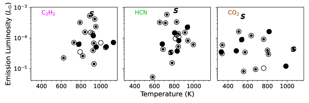
Figure 12: Median emission line luminosities from C₂H₂ (left), HCN (middle), and CO₂ (right) versus the median slab temperatures measured from the 100 best-fit slab models for each disk, with markers representing the sub-mm dust substructures listed in Table 2.3. The slab temperatures and emission line luminosities are not correlated for any of the three molecules (Spearman $\rho=0.006,0.07,-0.1$; $p=0.9,0.8,0.6$, respectively), implying that brighter emission lines do not necessarily originate in hotter gas.

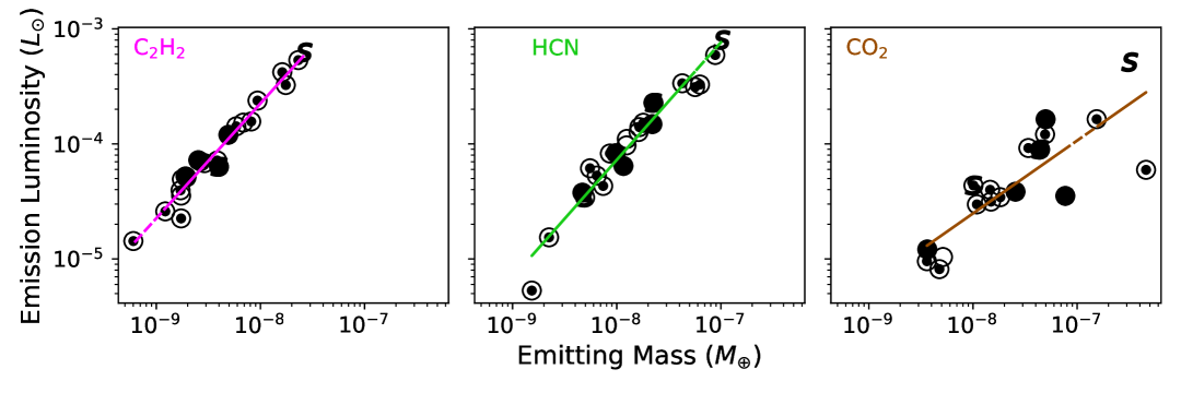
Figure 13: Median emission line luminosities from C₂H₂ (left), HCN (middle), and CO₂ (right) versus the median emitting masses measured from the best-fit slab models for each disk, with marker styles indicating the sub-mm dust substructures listed in Table 2.3. We report statistically significant, positive correlations and linear relationships between the two parameters for all three molecules (see Equation 1), implying that the emission is optically thin to moderately optically thick (Spearman $\rho=0.97,0.98,0.82$).

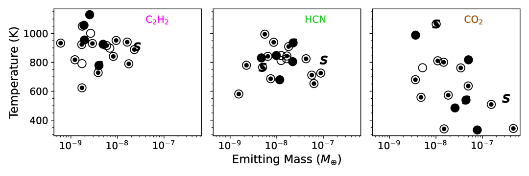
Figure 14: Retrieved temperatures from C₂H₂ (left), HCN (middle), and CO₂ (right) versus the median emitting masses measured from the best-fit slab models for each disk, with marker styles indicating the sub-mm dust substructures listed in Table 2.3. No significant correlations are observed for C₂H₂ or HCN (Spearman $\rho=-0.1,-0.04$; $p=0.6,0.8$), but we report a significant negative correlation between CO₂ temperature and emitting mass (Spearman $\rho=-0.55$; $p=0.02$).

Figure 15 shows the optical depth versus column density for all combinations of C₂H₂, HCN, and CO₂ slab model parameters that best reproduce the spectrum of AS 205N, confirming that the gas is optically thin and that the emission line strength is directly tracing the underlying warm molecular mass. The optical depths of C₂H₂ and HCN are always $\tau<1$, up to column densities of $\sim 10^{16}$ cm^-2. The CO₂ solutions exceed $\tau>1$ beyond $\sim 2\times 10^{16}$ cm^-2, tentatively indicating more optically thick emission. However, we note that the ¹³CO₂ $Q$ branch is not detected in AS 205N, indicating that the true column densities are likely more consistent with the smaller values (see e.g., Xie et al. 2023; Salyk et al. 2025). By contrast, $R>30000$ spectroscopy of H₂O in disks demonstrates that the gas is optically thick (see e.g., Banzatti et al. 2023b). In this work, we also report a weaker correlation between the H₂O emission line luminosities and emitting masses (Spearman $\rho=0.66$) than is observed for the C₂H₂, HCN, and CO₂ emission (Spearman $\rho=0.97,0.98,0.82$, respectively), which further supports this picture of optically thicker water and optically thinner organics.

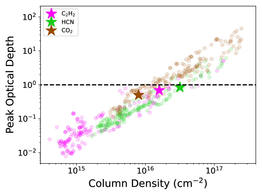
Figure 15: Optical depths versus column densities for the combinations of C₂H₂ (magenta), HCN (green), and CO₂ (brown) slab model parameters that best reproduce the spectrum of AS 205N; markers with stars correspond to the column densities used in Figure 7, and the black, dashed line shows $\tau=1$. In general, the C₂H₂ and HCN slab models are optically thin to larger column densities than the CO₂. We note that the ¹³CO₂ $Q$ branch near 15.4 $\mu$m is not detected in this target (see e.g., Grant et al. 2023; Xie et al. 2023; Salyk et al. 2025), or the ¹³C¹²CH₂ $Q$ branch seen in DoAr 33 and GO Tau (Tabone et al., 2023; Kanwar et al., 2024b; Arabhavi et al., 2024; Colmenares et al., 2024).

Table 9: Correlations Between Retrieval Parameters and Disk/Stellar Properties

Parameter	Molecule	$r_{\rm{dust}}$	$r_{\rm{inner}}$	$n_{13-26}$	$M_{\ast}$	$\dot{M}_{\rm{acc}}$	[Ne II] Flux	[Ne III]/[Ne II]
Line Luminosity	C2H2	-0.084	0.143	-0.538	0.367	0.642	0.583	0.250
	HCN	0.053	-0.015	-0.331	0.259	0.504	0.400	0.392
	CO2	0.034	0.221	-0.081	-0.106	0.503	0.569	-0.120
Temperature	C2H2	-0.540	-0.403	0.149	-0.207	0.064	0.005	0.821
	HCN	-0.107	0.009	0.136	-0.112	-0.240	-0.102	0.107
	CO2	0.109	0.200	-0.262	-0.156	0.479	-0.181	0.800
Emitting Mass	C2H2	-0.036	0.181	-0.531	0.381	0.675	0.590	0.321
	HCN	0.033	-0.033	-0.381	0.299	0.523	0.397	0.393
	CO2	-0.123	0.042	-0.076	-0.125	0.147	0.424	-0.300

4.2 Correlations Between Slab Model Parameters and Disk and Stellar Properties

Table 9 presents the Spearman rank coefficients between the emission line luminosities, slab temperatures, emitting masses, and the disk and stellar properties and atomic line fluxes included in Tables 2.3, 2.3, and 8. We do not identify any statistically significant correlations between the slab model temperatures and the radii of the innermost sub-mm dust rings, the infrared spectral indices, the mass accretion rates, or the [Ne II] emission line fluxes. There is a significant negative correlation between the C₂H₂ temperatures and the sub-mm disk radii (Spearman $\rho=-0.540$), indicating a cooler emitting layer in larger disks. However, the correlation is not present with the HCN or CO₂ emission line luminosities.

The most significant correlations are found between the emission line luminosities for all three molecules and the mass accretion rates, consistent with the Spitzer findings reported by Banzatti et al. (2020). We also report significant anti-correlations between the C₂H₂, HCN, and CO₂ luminosities and the infrared spectral indices, again consistent with Spitzer results reported in Banzatti et al. (2020), suggesting a depletion of warm molecular gas as the inner disk clears (see Figure 16). Although the [Ne II] fluxes reported here do not include all spatially extended emission contained within the MRS field-of-view, they are also significantly positively correlated with the mass accretion rates (Spearman $\rho=0.509$; $p=0.005$), as expected if the bulk of the outflowing emission originates in the high-velocity component identified from spectrally resolved line profiles (Pascucci et al., 2020). The emission line luminosities of C₂H₂ and CO₂ are also correlated with the integrated [Ne II] fluxes, and the C₂H₂ temperatures are correlated with the [Ne III]/[Ne II] flux ratios. These trends are discussed further in the following section.

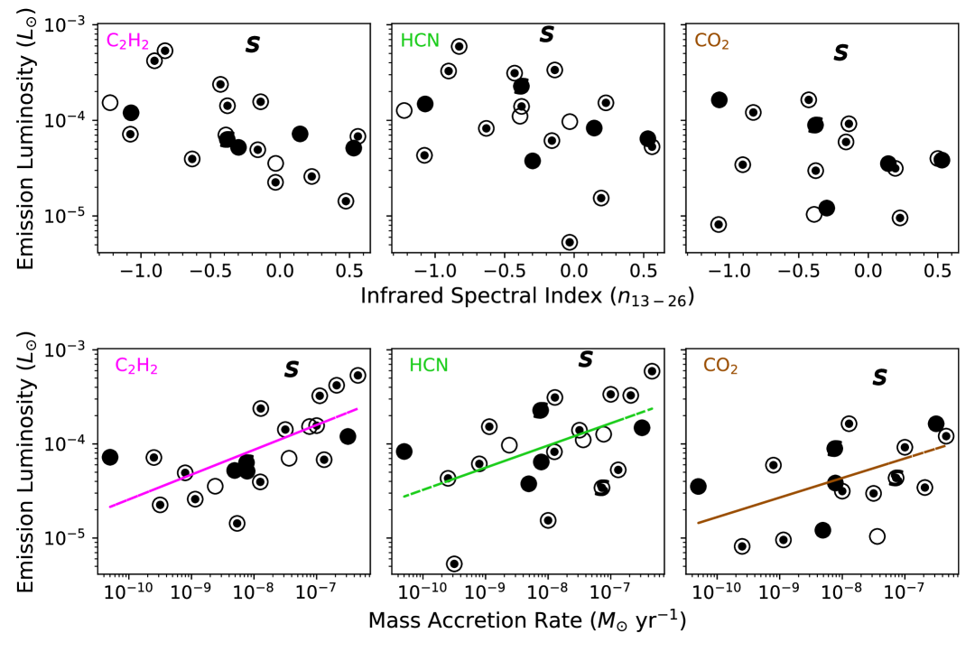
Figure 16: Emission line luminosities measured from the best-fit slab models versus the infrared spectral indices measured between 13 and 26 $\mu$m (top) and the literature mass accretion rates (bottom). Both trends are consistent with the Spitzer results reported in Banzatti et al. (2020).

5 Discussion

5.1 Can we observe the influence of outer disk substructures on inner disk chemistry?

As described in Section 3.1, sub-mm surveys at high angular resolution now provide a critical context for examining the impact of dust rings, gaps, cavities, and spiral arms on inner disk chemistry. Perhaps surprisingly, demographic studies with Spitzer found a connection between the MIR spectroscopic properties of disks (i.e., arising from the inner au) and their properties at millimeter wavelengths (i.e., arising from $>10$ au). In particular, the flux ratio of HCN to H₂O is found to generally increase with disk mass (Carr & Najita, 2011; Najita et al., 2013) and with the size of the dust disk at millimeter wavelengths (Banzatti et al., 2020).

Some of the diversity in the MIR spectra of T Tauri disks could be driven by planet formation processes through their impact on water transport in disks (Najita et al., 2013). While the formation of large, non-migrating, icy objects (planetesimals and larger objects) can sequester oxygen beyond the snow line, their associated substructures, created either as a consequence of planet formation (spiral arms, gaps, rings, cavities) or as precursors to it (dust traps; see e.g., Bae et al. 2023 and references therein), can also inhibit the inward drift of small icy solids to the inner disk (Kalyaan et al., 2021, 2023). In the case of multiple gaps within a single disk, the depth and radial location of the innermost gap remain the main factors that determine whether or not a disk is water-rich (Easterwood et al., 2024).

Because the general consequence of these planet formation processes is to inhibit inward water transport, disks in which these processes along with carbon grain destruction inside the soot line are active will tend to have higher C/O ratios in their inner disks (Kress et al., 2010; Carr & Najita, 2011; Najita et al., 2013; Booth et al., 2017; Booth & Ilee, 2019; Arabhavi et al., 2024; Colmenares et al., 2024). In contrast, disks that have not formed planets, contain leaky gaps, or otherwise have not trapped icy solids are likely to instead experience significant inward icy pebble drift, leading to an oxygen-rich inner disk (Banzatti et al., 2020; Kalyaan et al., 2021, 2023; Mah et al., 2024). At the same time, this evolutionary effect may not be apparent from the measured H₂O column densities alone if dust grains remain coupled to the gas inside the snowline; CO₂ is also required to trace the time evolution of the oxygen content (Sellek et al., 2025; Houge et al., 2025). In other words, disks that have engaged in planet formation processes to a greater or lesser extent may therefore manifest different inner disk chemical ratios.

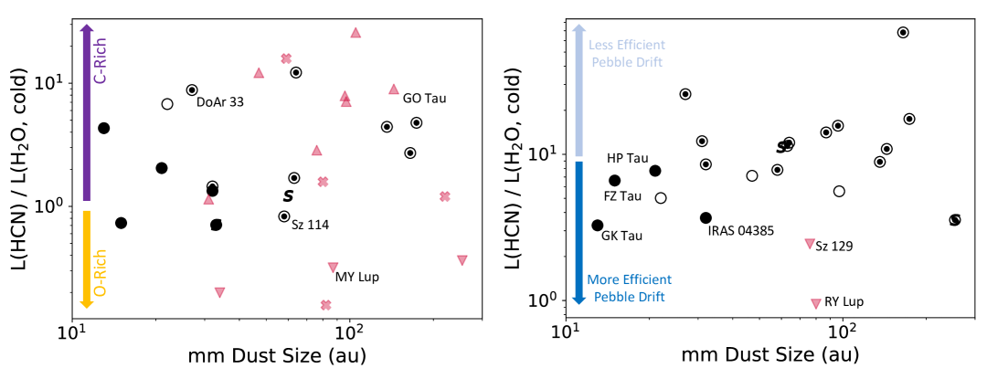
Figure 17: Left: Ratios of C₂H₂ to CO₂ integrated emission line luminosities versus sub-mm dust disk sizes from Table 2.3. Red markers denote lower limits for disks where CO₂ was not detected (VZ Cha, TW Cha, Sz 129, MWC 480), upper limits for disks where C₂H₂ was not detected (AS 205S, MY Lup, Elias 27), and Xs for disks where neither molecule was detected (RY Lup). Right: Ratios of HCN integrated emission line luminosities and cold 23.85 $\mu$m H₂O emission from (Banzatti et al., 2025) versus sub-mm dust disk size. Black markers are used to identify sub-mm substructures, as listed in Table 2.3.

In Figure 17, we compare the ratios of C₂H₂ and CO₂ integrated emission line luminosities to the sub-mm dust disk sizes reported in Table 2.3, using the markers listed in Table 2.3 to indicate the detected outer disk substructures. The two parameters are uncorrelated (Spearman $\rho=0.033$; $p=0.8$), indicating that the outer disk size alone does not determine whether the inner disk is more carbon-rich or oxygen-rich. No clear division is observed as a function of resolved substructures, and the line luminosities and radii of the innermost dust rings are also not correlated (see Table 9). We note that the closest resolved sub-mm dust rings in our sample are at $r\sim 6$ au (Huang et al., 2018a; Andrews et al., 2021), which is still well outside the expected zone of warm, mid-infrared molecular gas emission (see e.g., Anderson et al. 2021; Vlasblom et al. 2024). Further observations of smooth, compact disks, in addition to the four presented in this work, may help clarify this picture. Additional comparisons to 5 $\mu$m CO observations will also provide additional context for interpreting the carbon content within the inner regions of disks (Salyk et al., 2011a; Brown et al., 2013).

Figure 17 also compares the ratios of HCN and cold H₂O luminosities (the latter as adopted from Banzatti et al., 2025) to the sub-mm dust disk sizes reported in Table 2.3 (see also, Gasman et al. 2025). In multiple small disks in our sample, the observed H₂O emission from two transitions near $\sim 23.85$ $\mu$m is consistent with sublimation of icy pebbles ($T\sim 170$–220 K, see Banzatti et al., 2025), which may produce excess flux in transitions with low rotational excitation energies (Zhang et al., 2013; Banzatti et al., 2023a). While the small, smooth disks show similar C₂H₂-to-CO₂ emission line luminosity ratios to the larger disks with structures, they generally show less HCN emission relative to the cold H₂O luminosity (Spearman $\rho=0.36$; $p=0.11$). The trend weakens to Spearman $\rho=0.30$ and Spearman $\rho=0.18$ when the denominator is replaced with the warm and hot H₂O luminosities adopted from Banzatti et al. (2025), respectively. This again suggests that icy pebble drift is the mechanism driving the previously reported trend, producing an excess population of cold water vapor while leaving the warmer in situ water reservoirs unaffected.

We note that the strong correlation between $L_{\rm{HCN}}/L_{\rm{H_{2}O}}$ reported in Najita et al. (2011, 2013) focused on a sample with a narrower span of infrared spectral indices, age, and stellar metallicity than the stellar and disk properties of our sample. Now that the sensitivity of MIRI-MRS has enabled the detection of a thermal gradient in the observed water vapor (Banzatti et al., 2023a, 2025; Romero-Mirza et al., 2024a), it is possible to see the trend in a more diverse sample, although it is only marginally statistically significant. The prominent outliers in the $L_{\rm{HCN}}/L_{\rm{H_{2}O,\,cold}}$ correlation (Sz 129, Elias 27, RY Lup, two of which have an inner dust cavity) are disks that have relatively low HCN luminosities but still relatively high cold water fluxes (Banzatti et al., 2025). We also report that all disks smaller than $r<25$ au show $L_{\rm{HCN}}/L_{\rm{H_{2}O,\,cold}}<10$, again consistent with a picture where icy pebble drift proceeds more efficiently in compact systems and/or where ongoing planet formation has trapped oxygen in the outer disk. However, none of the four compact disks included in this work (HP Tau, FZ Tau, GK Tau, IRAS 04385) are particularly carbon-rich relative to the rest of the JDISCS sample, supporting the idea that the main driver of the correlation with disk radius is water itself (Banzatti et al., 2020, 2023a).

5.2 How common is optically thick emission from warm organics?

Optically thick molecular gas emission from deeper layers of the disk can produce a broad pseudo-continuum in the spectra, as the lines become wider than the instrument resolution and blend with adjacent transitions. This effect was recently confirmed in hydrocarbon emission for the first time, from a disk surrounding the very low mass star 2MASS J16053215-1933159 ($M_{\ast}=0.14\,M_{\odot}$; Tabone et al. 2023), as MIRI spectra were able to resolve the broadband feature first reported from Spitzer observations (Pascucci et al., 2013). The emission is consistent with the superposition of optically thick and thin C₂H₂ components, one with column density $N\rm{\left(C_{2}H_{2}\right)}=2.4\times 10^{20}$ cm^-2 and $T=525$ K and the other with column density $N\rm{\left(C_{2}H_{2}\right)}=2.5\times 10^{17}$ cm^-2 and $T=400$ K (Tabone et al., 2023; Arabhavi et al., 2024). Such prominent, optically thick emission was attributed to increased destruction of carbon-bearing grains at the “soot” line, which may proceed more efficiently as dust settling allows UV photons to travel deeper into the molecular gas layer (see also, Colmenares et al. 2024). However, in most C-rich disks around very low mass stars, the hydrocarbon excitation temperature is much lower than the temperature at the “soot” line, indicating that this effect alone cannot fully explain the excess carbon content (Long et al., 2025). In any case, such features can be removed by iterative continuum fitting processes such as those described in Section 2, shifting the retrieved column densities to smaller values as a result.

While none of our sources show a broad pseudo-continuum near 13.7 $\mu$m that is as prominent as the features detected in the spectra of 2MASS J16053215-1933159 (Pascucci et al., 2013; Tabone et al., 2023), Sz 28 (Kanwar et al., 2024b), ISO-ChaI 147 (Arabhavi et al., 2024), or the 30 Myr disk WISE J044634.16–262756.1B (Long et al., 2025), we identify a subset of disks in Figure 9 that require larger C₂H₂ slab temperatures to reproduce the spectra ($T\sim 1000$ K). Most are relatively compact, with sub-mm dust disk radii between $r=13-58$ au). Figure 18 highlights these targets, showing “pedestals” under the C₂H₂ and HCN $Q$-branch emission that are narrower than the broad pseudo-continuum observed in carbon-rich disks but still do not fall flat against the dust continuum (GK Tau, FZ Tau, HP Tau, GQ Lup, and Sz 114; see also Xie et al. 2023). Clear signatures of excess cold water emission at longer wavelengths that we do not model here are also detected (Banzatti et al., 2023a; Romero-Mirza et al., 2024a; Banzatti et al., 2025; Gasman et al., 2025). We compare the residuals from our slab model fits to scaled, optically thick slab models with $\log N_{\rm{col}}=22$ cm^-2 and $T=525$ K (Tabone et al., 2023; Arabhavi et al., 2024), to explore whether an additional C₂H₂ component can fill in the missing flux. However, the optically thick models clearly over-predict the fluxes in the $P$ and $R$ branch emission lines at wavelengths further from the bandhead.

Although some calibration issues complicated analysis between $\sim 13-15$ $\mu$m in early JWST observations (Chown et al., 2024), the JDISCS pipeline has improved this considerably (Pontoppidan et al., 2024). Since only a subset of disks in our sample show the “pedestals”, it is also unlikely that the features can be attributed to the continuum subtraction routine described in Section 2.3; instead, we consider other mechanisms that may be responsible for the excess emission. There are no expected PAH features in the 13.7 $\mu$m region (Sloan et al., 2014; Jones et al., 2023), although this broad feature has long been noted in absorption toward embedded sources such as IRc2 in Orion (e.g. Evans et al., 1991). Evans et al. (1991) attributed this to material in front of the hot protostellar core or the plateau feature in that region, in which emitting and absorbing material could have been co-located by line-of-sight. Alternatively, the excess emission also overlaps with double-peaked pyroxene features that were tentatively detected with Spitzer at 13.6, 14.5, and 15.5 $\mu$m toward Class II disks (Chihara et al., 2002; Carr & Najita, 2011), where the Fe concentration determined the peak wavelengths and shapes of the observed bands. However, a full treatment of the corresponding 10 $\mu$m silicate emission will be required to reproduce these features and is beyond the scope of this work. We conclude that the excess “pedestal” under the organic emission in the small disks is not consistent with an optically thick gas pseudo-continuum emerging from deeper in the disk and may instead be attributed to dust emission, implying that the prominent bumps presented in previous works are unique features even among compact disks (Tabone et al., 2023; Kanwar et al., 2024b; Arabhavi et al., 2024; Long et al., 2025). As current state-of-the-art techniques for simultaneous modeling of dust and molecular gas emission (see e.g., Kaeufer et al. 2024a) have not yet been demonstrated on faint signatures such as those reported here, updated models of the dust continuum will be required to obtain the best constraints on the temperature structure of the mid-infrared disk layers.

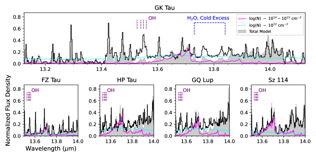
Figure 18: Subset of JDISCS Cycle 1 targets with retrieved C₂H₂ slab temperatures of $\sim$1000 K, required to reproduce broader “pedestal”-like emission than observed in the other disks from our sample (magenta; full models from Figure 4 are filled in gray). Optically thick C₂H₂ components with $\log N=22$ cm^-2 are over-plotted for comparison (cyan; Tabone et al. 2023; Arabhavi et al. 2024), and OH emission lines that were not included in our fits are marked with purple, dashed lines. While the optically thick gas models can reproduce the excess emission near the bandheads, they overpredict the emission from the $P$ and $R$ branch transitions and are therefore not consistent with the overall shapes of the pedestals.

5.3 How does inner disk chemistry evolve with accretion and disk dispersal?

[Ne II], [Ne III], and [Ar II] emission lines are expected to trace either high-velocity winds/microjets in disks that are strong accretors ($M_{\rm{acc}}>10^{-8}\,M_{\odot}$; Pascucci et al. 2020) or low-velocity winds otherwise (Hollenbach & Gorti, 2009; Espaillat et al., 2013; Sellek et al., 2024). Photoevaporative wind models predict that [Ne III]/[Ne II] flux ratios will be $<1$ when X-ray irradiation dominates the disk ionization and dispersal processes, while ratios $>1$ are consistent with EUV driven wind models (Hollenbach & Gorti, 2009; Espaillat et al., 2013; Bajaj et al., 2024). A [Ne II]/[Ar II] ratio $<2.5$ is expected under an EUV or soft X-ray radiation field, while [Ne II]/[Ar II] $>2.5$ points to a hard X-ray spectrum (Espaillat et al., 2023). Alternatively, a UV dominant spectrum would trigger gas-phase reactions in hotter layers; this effect may be particularly apparent in the OH-H₂O formation pathways (Agúndez et al., 2008; Ádámkovics et al., 2014, 2016; Walsh et al., 2015). Since the C₂H₂, HCN, and CO₂ emission is generally optically thin (see Figure 13) and therefore directly exposed to stellar and accretion-generated radiation, understanding the mechanisms driving the Ne and Ar ionization may also constrain the high-energy flux that catalyzes photochemistry in the warm molecular gas (see e.g., Agúndez et al. 2008; Pascucci et al. 2009; Najita et al. 2011; Szulágyi et al. 2012; Walsh et al. 2015; Gaidos et al. 2025).

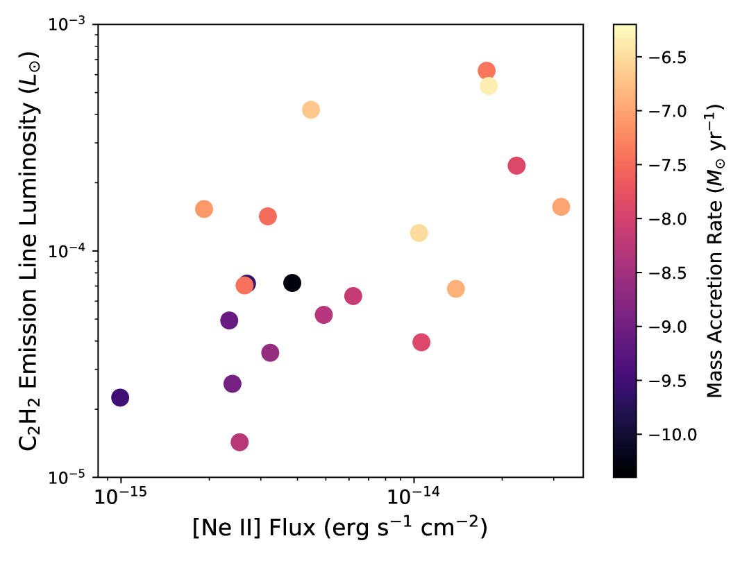
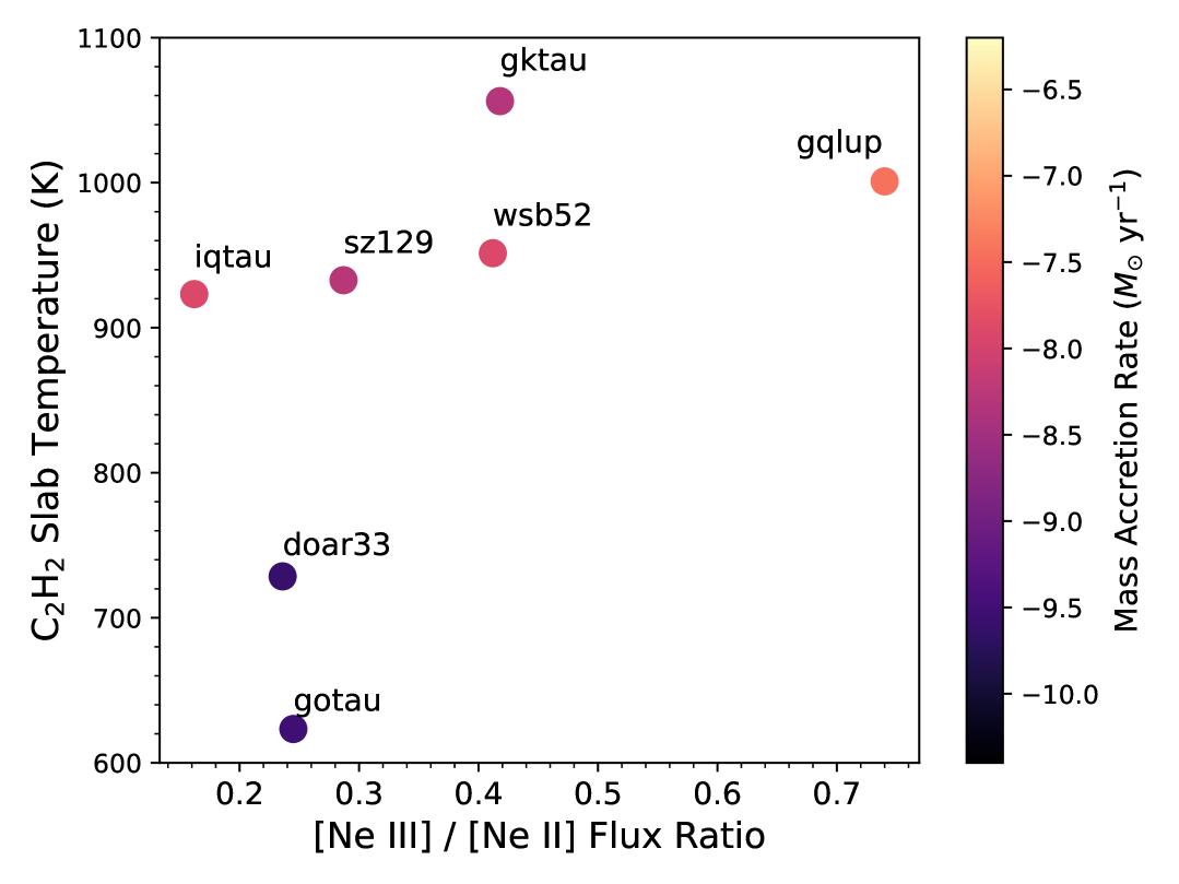
Figure 19: Left: C₂H₂ emission line luminosities versus [Ne II] emission line fluxes. Right: C₂H₂ slab temperatures versus [Ne III] to [Ne II] flux ratios. In both panels, marker colors represent mass accretion rates (see also, Colmenares et al. 2024). Upper limits are omitted from the plot and correlation coefficient calculation (see Table 9), due to the large uncertainty in the water removal at 15.555 $\mu$m.

All ten JDISCS targets with [Ne III] detections show [Ne III]/[Ne II] ratios $<1$, with a range from 0.1 (MY Lup) to 0.7 (GQ Lup), placing them all in the X-ray irradiation regime. This is consistent with results from Spitzer, where [Ne III]/[Ne II] $>1$ was never detected (Najita et al., 2010; Espaillat et al., 2013; Bajaj et al., 2024). For the [Ar II] detections, we find that MY Lup, GM Aur, and IQ Tau have [Ne II]/[Ar II] $>2.5$ and HD 143006, MWC 480, and RY Lup $<2.5$. In MY Lup, GM Aur, and IQ Tau, the combination of $\rm{[Ne\,III]/[Ne\,II]}=0.1-0.2$ and $\rm{[Ne\,II]/[Ar\,II]}>2.5$ is consistent with hard X-ray spectra reaching the disks (Szulágyi et al., 2012). These radiation fields may drive gas-phase chemistry via ion-neutral reactions in cooler, UV-shielded disk layers (see e.g., Agúndez et al. 2008; Najita et al. 2011; Walsh et al. 2015).

MY Lup and IQ Tau both have similar sub-mm dust disk sizes (see Figure 3; $r_{\rm{dust}}=87,96$ au for MY Lup, IQ Tau, respectively; Huang et al. 2018a; Long et al. 2019a), and GM Aur has a much larger disk ($r_{\rm{dust}}=220$ au; Huang et al. 2020) and a prominent dust cavity. Despite the similarity of their atomic features, the molecular emission spectra from all three targets do not show any clear grouping. MY Lup is one of the most distinctive targets in JDISCS, showing ¹²CO₂ with a peak/continuum ratio of $\sim 0.1$ and clear detections of C¹⁸O¹⁶O and H¹³CN (Salyk et al., 2025). However, CO₂ is not detected at all in IQ Tau (peak/continuum $<0.02$) or GM Aur (peak/continuum $<0.03$). Similarly, C₂H₂ is detected in IQ Tau with a peak/continuum ratio of $\sim 0.06$ but not detected in MY Lup or GM Aur (peak/continuum $<0.03$). It is possible that the line-of-sight toward IQ Tau probes a layer of gas with lower column densities than that toward MY Lup (Salyk et al., 2025). Identification of additional disks with organics-rich spectra and signatures of wind-driven inner disk clearing, i.e. pre-transitional disks, will be required to further explore this connection.

Of the three organic molecules presented here, C₂H₂ shows the strongest evidence for a potential link between inner disk molecular gas emission and the MHD or photoevaporative wind-driven ionization structure across our sample (see Figure 19). We find that the C₂H₂ emission line luminosities and emitting masses are significantly positively correlated with the [Ne II] fluxes ($\rho=0.583,0.590$, respectively; see Figure 19 for emission line luminosities and [Ne II] fluxes), which in turn are expected to scale with X-ray luminosity in static disk models with low EUV flux (Hollenbach & Gorti, 2009; Pascucci et al., 2014). Meanwhile, the C₂H₂ slab temperatures are also significantly positively correlated with the [Ne III]/[Ne II] flux ratios ($\rho=0.821$), indicating that the molecular layer becomes hotter as EUV heating becomes more significant. As reported by Banzatti et al. (2017, 2020) from analyses of Spitzer spectra, we also find positive correlations between the mass accretion rates and C₂H₂, HCN, and CO₂ emission line luminosities ($\rho=0.642,0.504,0.503$, respectively), as expected if UV photons generated at the accretion shocks are responsible for heating the gas. A new interesting aspect to explore in future work is emerging from studies of accretion variability and outbursts, which can increase/decrease the observed molecular fluxes in different phases of accretion due to disk heating and UV photo-dissociation (Banzatti et al. (2012), Smith et al. 2025, in press).

However, only a small subset of targets have C₂H₂, [Ne III], and [Ne II] detections. Further clarification of this trend will require a more complete inventory of water emission lines across the full MIRI wavelength range, to place well-constrained upper limits on the [Ne III] emission. Complementary observations at FUV through X-ray wavelengths will also reveal the radiation fields generated by the accreting host stars, constraining the flux received at the disk surfaces. We note again that the aperture used to extract the 1-D spectra presented in this work does not capture spatially extended emission from the atomic wind tracers, which may in turn alter the reported flux ratios. An exploration of spatially extended emission across the JDISCS sample is forthcoming (Pontoppidan et al., in prep).

6 Conclusions

As observations of protoplanetary disks with JWST MIRI are ongoing, JDISCS is providing a database of consistently reduced, high-quality mid-infrared spectra that enable inner disk population studies. From this database, we present an overview of H₂O, C₂H₂, HCN, CO₂, [Ne II], [Ne III], and [Ar II] emission lines from the 31 JDISCS systems observed in Cycle 1. Although this initial sample probes only a small range in stellar mass, spectra show approximately two orders of magnitude variation in molecular line luminosities. H₂O and OH emission is nearly ubiquitous, and detection rates are higher for MRS than they were for Spitzer-IRS.

We fit LTE slab models to the spectra to retrieve column densities, temperatures, and emitting areas for three organic molecules and water at 12–16 $\mu$m, finding that:

• Emission line luminosities are significantly correlated with the molecular emitting masses of C₂H₂, HCN, and CO₂, but they are not correlated with the slab temperatures.

• CO₂ emission generally comes from cooler, more optically thick gas $\left(T=600^{+200}_{-160}\,\rm{K}\right)$ than C₂H₂ and HCN emission ($T=920^{+70}_{-130},820^{+70}_{-130}$ K, respectively).

These results confirm that C₂H₂, HCN, and CO₂ emission lines are generally optically thin to moderately optically thick, originating in warm surface layers of the inner disk.

All targets included in this work were previously observed with ALMA at high angular resolution, and we consider the impact of outer disk substructures on the molecular gas emission. We identify the following trends from our analysis:

• Excess emission is visible as a “pedestal” under the C₂H₂ and HCN $Q$ branches in the smallest disks, but it is not consistent with optically thick emission from deeper disk layers (see e.g., Tabone et al. 2023; Arabhavi et al. 2024; Long et al. 2025). This “pedestal” emission drives the retrieved C₂H₂ temperatures higher than in other disks ($T>1000$ K) and is likely due to dust features.

• The ratios of C₂H₂ to CO₂ emitting masses are not correlated with sub-mm disk sizes, indicating that disk size alone does not necessarily determine the ratios of carbon- and oxygen-bearing molecules (Colmenares et al., 2024).

• Smaller disks generally have larger fluxes from cold H₂O relative to HCN, consistent with a picture where either pebble drift and its impediment by dust traps regulates water delivery to the inner disk (Banzatti et al., 2020, 2023a; Gasman et al., 2025) or where advanced planet formation has sequestered oxygen in more massive disks (Najita et al., 2013).

Finally, we examine the brightest atomic forbidden emission lines, finding that:

• $\left[\rm{Ne\,II}\right]$ is detected in all but three disks included in this work, [Ne III] in ten sources, and [Ar II] in four systems.

• The measured [Ne III]/[Ne II] emission line fluxes are all $<1$, consistent with X-ray irradiation as the primary ionization source (Espaillat et al., 2023; Bajaj et al., 2024).

• The [Ne II]/[Ar II] flux ratios indicate that the disks around MY Lup, IQ Tau, and GM Aur receive a hard X-ray spectrum, which may influence gas-phase chemistry in the optically thin emitting layers.

While this study provides a first step toward a global analysis of atomic and molecular spectra from a sample of disks observed with MRS, the targets analyzed in this work are limited to stellar masses around solar and ages of a few Myr. Additional JDISCS programs are underway to better probe trends with stellar mass and disk evolutionary state. A more comprehensive treatment of the molecular gas across the entire MRS spectrum must also include the addition of less abundant species and isotopologues (e.g., ¹³C¹²CH₂, C₄H₂, C¹⁸O¹⁶O, H¹³CN; Tabone et al. 2023; Kanwar et al. 2024b; Colmenares et al. 2024; Salyk et al. 2025), fit simultaneously to distinguish between overlapping transitions. Such efforts may require the adaptation of machine learning techniques that are not yet widely applied to spectra of protoplanetary disks, in order to capture the most relevant physics while minimizing computation time (see e.g., Diop et al. 2024; Kaeufer et al. 2024b). However, the initial findings presented here highlight the potential of MIRI MRS to reveal demographic trends and links between the physics and chemistry of inner and outer protoplanetary disk zones.

We thank the referee for a thorough review that greatly contributed to the clarity of the paper. A portion of this research was carried out at the Jet Propulsion Laboratory, California Institute of Technology, under a contract with the National Aeronautics and Space Administration (80NM0018D0004).

Appendix A Impact of Water Removal on Slab Model Fits to Organics in MIRI-MRS Spectra

The wavelength range in which HCN, C₂H₂, and CO₂ are detected in our MIRI-MRS spectra also includes a large number of rotational emission lines from the ground state and first excited state bending mode manifold of H₂O (see e.g., Banzatti et al. 2023a; Grant et al. 2023; Gasman et al. 2023; Xie et al. 2023; Pontoppidan et al. 2024; Romero-Mirza et al. 2024a). These water lines must be subtracted in order to model the organics, to ensure that emission across the full rotational ladder within each vibrational band can be used to constrain the temperature of the emitting region. Previous work has achieved this by using scale factors to predict the water flux near the HCN $Q$ branch emission (see e.g., Najita et al. 2013) or by fitting the water emission lines in other regions of the spectra with single temperature slab models (see e.g., Salyk et al. 2011b; Grant et al. 2023).

The single temperature slab model fits to Spitzer-IRS observations were generally consistent with a population of H₂O with $T\sim 450$ K and $N\sim 10^{18}$ cm^-2 (Carr & Najita, 2008; Salyk et al., 2011b). However, at the higher spectral resolving power of the MRS ($R\sim 2250-2725$ between 13-14.5 $\mu$m; Pontoppidan et al. 2024), two ground state populations of H₂O with $T\sim 800$ and $T=370-500$ K have been detected in several compact disks where efficient icy pebble drift produces excess emission from sublimated gas near the water snowline (Banzatti et al., 2023b). Notably, the cooler excess emission is not detected in larger disks where icy pebbles are likely trapped within dust rings (Kalyaan et al., 2021, 2023). It is now possible to include multiple temperature components to reproduce the spectra (see e.g., Romero-Mirza et al. 2024a; Grant et al. 2024).

These two component slab model fits, or radial gradient retrievals (Romero-Mirza et al., 2024a), typically assume LTE excitation of all ro-vibrational states. Building on this effort, Banzatti et al. (2025) reveals that the rovibrational band near 6 $\mu$m and the pure rotational hot band lines at longer wavelengths are suppressed compared to LTE. Here we do not consider the rovibrational emission, and note that the hot band $v=1-1$ rotational emission flux is weak compared to the ground state lines. Thus, we also do not consider these further in the present analysis. For more precise fits to individual sources, distinct but constant mutliplicative factors for the rovibrational and hot band rotational emission lines can be used as a first order characterization of the water vapor emission (Banzatti et al., 2025).

Since the water emission lines that show the strongest signatures of multiple temperature components are generally weaker in the 12-16 $\mu$m wavelength range where HCN, C₂H₂ and CO₂ emission is observed, we use single temperature slab models to reproduce and subtract the H₂O emission. All retrieved parameters are reported in Table 10.

Table 10: Slab Model Fit Parameters: H₂O, Rotational lines at 12–16 $\mu$m

Target	$\log N$	$r_{\text{slab}}$	$M_{\text{emit}}$	$T$	$L_{\text{emit}}$	P/C
	(cm-2)	(au)	$\log M$ ($M_{\oplus}$)	(K)	$\log L$ ($L_{\odot}$)
AS 205 N	18.7	1.6	-4.4	$610\pm 5$	-2.4	0.22
AS 205 S	17.6	1.3	-5.6	$530\pm 10$	-3.6	0.08
AS 209	19.5	0.2	-5.8	$890\pm 10$	-3.3	0.04
CI Tau	18.3	0.4	-6.1	$880\pm 10$	-3.2	0.27
DoAr 25	18.8	0.3	-5.9	$640\pm 10$	-3.8	0.14
DoAr 33	18.8	0.2	-6.0	$610^{+20}_{-10}$	-4.0	0.11
Elias 20	18.5	0.7	-5.3	$640\pm 10$	-3.1	0.34
Elias 24	18.4	1.2	-4.9	$600\pm 10$	-2.8	0.29
Elias 27	18.5	0.5	-5.6	$640\pm 10$	-3.4	0.54
FZ Tau	18.5	0.8	-5.1	$690\pm 10$	-2.8	0.53
GK Tau	18.1	0.3	-6.3	$760\pm 10$	-3.6	0.10
GM Aur	17.8	0.2	-6.6	$480\pm 50$	-5.0	0.03
GO Tau	17.8	0.2	-7.2	$570\pm 20$	-5.0	0.06
GQ Lup	17.8	0.7	-6.0	$620\pm 10$	-3.6	0.12
HD 142666	$\cdots$	$\cdots$	$<-5.7$	$\cdots$	$<-5.3$	$<10^{-3}$
HD 143006	$\cdots$	$\cdots$	$<-6.8$	$\cdots$	$<-4.3$	$<0.01$
HD 163296	$\cdots$	$\cdots$	$\cdots$	$\cdots$	$\cdots$	$\cdots$
HP Tau	18.2	0.3	-6.2	$760\pm 10$	-3.5	0.05
HT Lup	18.7	0.3	-5.6	$790\pm 10$	-3.2	0.06
IQ Tau	18.4	0.2	-6.5	$910^{+20}_{-10}$	-3.6	0.15
IRAS 04385	18.5	0.6	-5.4	$530\pm 10$	-3.6	0.15
MWC 480	18.8	0.2	-5.9	$870^{+60}_{-10}$	-3.4	0.01
MY Lup	18.5	0.3	-5.9	$390\pm 10$	-4.8	0.02
RU Lup	18.2	0.9	-5.3	$730\pm 10$	-2.7	0.19
RY Lup	17.6	0.4	-6.7	$530\pm 10$	-4.6	0.009
SR 4	18.1	0.3	-6.4	$840\pm 10$	-3.5	0.10
Sz 114	18.7	0.4	-5.5	$580\pm 10$	-3.7	0.26
Sz 129	18.0	0.3	-6.5	$750\pm 10$	-3.8	0.24
TW Cha	18.1	0.5	-6.0	$740\pm 10$	-3.4	0.47
VZ Cha	18.1	0.5	-6.1	$840\pm 10$	-3.2	0.38
WSB 52	18.8	1.4	-4.3	$500\pm 5$	-2.9	0.73

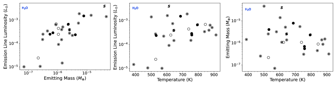
Figure 21: Correlations between best-fit parameters retrieved from single temperature slab model fits to H₂O emission lines between 12-17.5 $\mu$m. Although statistically significant, the correlation between emission line luminosities and emitting masses (left) is significantly weaker (Spearman $\rho=0.66$; $p=10^{-4}$) than what is observed for C₂H₂, HCN, and CO₂ (see Figure 8). The single slab temperatures are not correlated with either the emission line luminosities (middle; Spearman $\rho=0.35$; $p=0.064$) or emitting masses (right; Spearman $\rho=-0.24$; $p=0.21$).

References

- Ádámkovics et al. (2014) Ádámkovics, M., Glassgold, A. E., & Najita, J. R. 2014, ApJ, 786, 135, doi: 10.1088/0004-637X/786/2/135
- Ádámkovics et al. (2016) Ádámkovics, M., Najita, J. R., & Glassgold, A. E. 2016, ApJ, 817, 82, doi: 10.3847/0004-637X/817/1/82
- Agúndez et al. (2008) Agúndez, M., Cernicharo, J., & Goicoechea, J. R. 2008, A&A, 483, 831, doi: 10.1051/0004-6361:20077927
- Alcalá et al. (2019) Alcalá, J. M., Manara, C. F., France, K., et al. 2019, A&A, 629, A108, doi: 10.1051/0004-6361/201935657
- Alcalá et al. (2017) Alcalá, J. M., Manara, C. F., Natta, A., et al. 2017, A&A, 600, A20, doi: 10.1051/0004-6361/201629929
- Anderson et al. (2021) Anderson, D. E., Blake, G. A., Cleeves, L. I., et al. 2021, ApJ, 909, 55, doi: 10.3847/1538-4357/abd9c1
- Andrews et al. (2018) Andrews, S. M., Huang, J., Pérez, L. M., et al. 2018, ApJ, 869, L41, doi: 10.3847/2041-8213/aaf741
- Andrews et al. (2021) Andrews, S. M., Elder, W., Zhang, S., et al. 2021, ApJ, 916, 51, doi: 10.3847/1538-4357/ac00b9
- Ansdell et al. (2016) Ansdell, M., Williams, J. P., van der Marel, N., et al. 2016, ApJ, 828, 46, doi: 10.3847/0004-637X/828/1/46
- Arabhavi et al. (2024) Arabhavi, A. M., Kamp, I., Henning, T., et al. 2024, Science, 384, 1086, doi: 10.1126/science.adi8147
- Arulanantham et al. (2024) Arulanantham, N., McClure, M. K., Pontoppidan, K., et al. 2024, ApJ, 965, L13, doi: 10.3847/2041-8213/ad35c9
- Astropy Collaboration et al. (2013) Astropy Collaboration, Robitaille, T. P., Tollerud, E. J., et al. 2013, A&A, 558, A33, doi: 10.1051/0004-6361/201322068
- Astropy Collaboration et al. (2018) Astropy Collaboration, Price-Whelan, A. M., Sipőcz, B. M., et al. 2018, AJ, 156, 123, doi: 10.3847/1538-3881/aabc4f
- Astropy Collaboration et al. (2022) Astropy Collaboration, Price-Whelan, A. M., Lim, P. L., et al. 2022, ApJ, 935, 167, doi: 10.3847/1538-4357/ac7c74
- Bae et al. (2023) Bae, J., Isella, A., Zhu, Z., et al. 2023, in Astronomical Society of the Pacific Conference Series, Vol. 534, Protostars and Planets VII, ed. S. Inutsuka, Y. Aikawa, T. Muto, K. Tomida, & M. Tamura, 423, doi: 10.48550/arXiv.2210.13314
- Bajaj et al. (2024) Bajaj, N. S., Pascucci, I., Gorti, U., et al. 2024, AJ, 167, 127, doi: 10.3847/1538-3881/ad22e1
- Banzatti et al. (2019) Banzatti, A., Pascucci, I., Edwards, S., et al. 2019, ApJ, 870, 76, doi: 10.3847/1538-4357/aaf1aa
- Banzatti et al. (2017) Banzatti, A., Pontoppidan, K. M., Salyk, C., et al. 2017, ApJ, 834, 152, doi: 10.3847/1538-4357/834/2/152
- Banzatti et al. (2012) Banzatti, A., Meyer, M. R., Bruderer, S., et al. 2012, ApJ, 745, 90, doi: 10.1088/0004-637X/745/1/90
- Banzatti et al. (2020) Banzatti, A., Pascucci, I., Bosman, A. D., et al. 2020, ApJ, 903, 124, doi: 10.3847/1538-4357/abbc1a
- Banzatti et al. (2022) Banzatti, A., Abernathy, K. M., Brittain, S., et al. 2022, AJ, 163, 174, doi: 10.3847/1538-3881/ac52f0
- Banzatti et al. (2023a) Banzatti, A., Pontoppidan, K. M., Carr, J. S., et al. 2023a, ApJ, 957, L22, doi: 10.3847/2041-8213/acf5ec
- Banzatti et al. (2023b) Banzatti, A., Pontoppidan, K. M., Pére Chávez, J., et al. 2023b, AJ, 165, 72, doi: 10.3847/1538-3881/aca80b
- Banzatti et al. (2025) Banzatti, A., Salyk, C., Pontoppidan, K. M., et al. 2025, AJ, 169, 165, doi: 10.3847/1538-3881/ada962
- Booth et al. (2017) Booth, R. A., Clarke, C. J., Madhusudhan, N., & Ilee, J. D. 2017, MNRAS, 469, 3994, doi: 10.1093/mnras/stx1103
- Booth & Ilee (2019) Booth, R. A., & Ilee, J. D. 2019, MNRAS, 487, 3998, doi: 10.1093/mnras/stz1488
- Bosman et al. (2022) Bosman, A. D., Bergin, E. A., Calahan, J., & Duval, S. E. 2022, ApJ, 930, L26, doi: 10.3847/2041-8213/ac66ce
- Brown et al. (2013) Brown, J. M., Pontoppidan, K. M., van Dishoeck, E. F., et al. 2013, ApJ, 770, 94, doi: 10.1088/0004-637X/770/2/94
- Brown et al. (2007) Brown, J. M., Blake, G. A., Dullemond, C. P., et al. 2007, ApJ, 664, L107, doi: 10.1086/520808
- Brownlee et al. (2006) Brownlee, D., Tsou, P., Aléon, J., et al. 2006, Science, 314, 1711, doi: 10.1126/science.1135840
- Carr & Najita (2008) Carr, J. S., & Najita, J. R. 2008, Science, 319, 1504, doi: 10.1126/science.1153807
- Carr & Najita (2011) —. 2011, ApJ, 733, 102, doi: 10.1088/0004-637X/733/2/102
- Carr & Najita (2014) —. 2014, ApJ, 788, 66, doi: 10.1088/0004-637X/788/1/66
- Chihara et al. (2002) Chihara, H., Koike, C., Tsuchiyama, A., Tachibana, S., & Sakamoto, D. 2002, A&A, 391, 267, doi: 10.1051/0004-6361:20020791
- Chown et al. (2024) Chown, R., Sidhu, A., Peeters, E., et al. 2024, A&A, 685, A75, doi: 10.1051/0004-6361/202346662
- Cieza et al. (2010) Cieza, L. A., Schreiber, M. R., Romero, G. A., et al. 2010, ApJ, 712, 925, doi: 10.1088/0004-637X/712/2/925
- Colmenares et al. (2024) Colmenares, M. J., Bergin, E., Salyk, C., et al. 2024, arXiv e-prints, arXiv:2410.18187. https://arxiv.org/abs/2410.18187
- Diop et al. (2024) Diop, A., Cleeves, L. I., Anderson, D. E., Pegues, J., & Plunkett, A. 2024, ApJ, 962, 90, doi: 10.3847/1538-4357/ad11ed
- Donati et al. (2024) Donati, J. F., Finociety, B., Cristofari, P. I., et al. 2024, MNRAS, 530, 264, doi: 10.1093/mnras/stae675
- Drażkowska & Alibert (2017) Drażkowska, J., & Alibert, Y. 2017, A&A, 608, A92, doi: 10.1051/0004-6361/201731491
- Dullemond et al. (2018) Dullemond, C. P., Birnstiel, T., Huang, J., et al. 2018, ApJ, 869, L46, doi: 10.3847/2041-8213/aaf742
- Easterwood et al. (2024) Easterwood, W., Kalyaan, A., & Banzatti, A. 2024, ApJ, 977, 21, doi: 10.3847/1538-4357/ad891d
- Eisner et al. (2005) Eisner, J. A., Hillenbrand, L. A., White, R. J., Akeson, R. L., & Sargent, A. I. 2005, ApJ, 623, 952, doi: 10.1086/428828
- Espaillat et al. (2013) Espaillat, C., Ingleby, L., Furlan, E., et al. 2013, ApJ, 762, 62, doi: 10.1088/0004-637X/762/1/62
- Espaillat et al. (2023) Espaillat, C. C., Thanathibodee, T., Pittman, C. V., et al. 2023, ApJ, 958, L4, doi: 10.3847/2041-8213/ad023d
- Evans et al. (1991) Evans, Neal J., I., Lacy, J. H., & Carr, J. S. 1991, ApJ, 383, 674, doi: 10.1086/170824
- Fairlamb et al. (2015) Fairlamb, J. R., Oudmaijer, R. D., Mendigutía, I., Ilee, J. D., & van den Ancker, M. E. 2015, MNRAS, 453, 976, doi: 10.1093/mnras/stv1576
- Fang et al. (2018) Fang, M., Pascucci, I., Edwards, S., et al. 2018, ApJ, 868, 28, doi: 10.3847/1538-4357/aae780
- Fedele et al. (2012) Fedele, D., Bruderer, S., van Dishoeck, E. F., et al. 2012, A&A, 544, L9, doi: 10.1051/0004-6361/201219615
- Foreman-Mackey et al. (2013) Foreman-Mackey, D., Hogg, D. W., Lang, D., & Goodman, J. 2013, PASP, 125, 306, doi: 10.1086/670067
- Francis & van der Marel (2020) Francis, L., & van der Marel, N. 2020, ApJ, 892, 111, doi: 10.3847/1538-4357/ab7b63
- Frasca et al. (2017) Frasca, A., Biazzo, K., Alcalá, J. M., et al. 2017, A&A, 602, A33, doi: 10.1051/0004-6361/201630108
- Furlan et al. (2009) Furlan, E., Watson, D. M., McClure, M. K., et al. 2009, ApJ, 703, 1964, doi: 10.1088/0004-637X/703/2/1964
- Gaia Collaboration et al. (2016) Gaia Collaboration, Prusti, T., de Bruijne, J. H. J., et al. 2016, A&A, 595, A1, doi: 10.1051/0004-6361/201629272
- Gaia Collaboration et al. (2018) Gaia Collaboration, Brown, A. G. A., Vallenari, A., et al. 2018, A&A, 616, A1, doi: 10.1051/0004-6361/201833051
- Gaia Collaboration et al. (2021) —. 2021, A&A, 649, A1, doi: 10.1051/0004-6361/202039657
- Gaia Collaboration et al. (2023) Gaia Collaboration, Vallenari, A., Brown, A. G. A., et al. 2023, A&A, 674, A1, doi: 10.1051/0004-6361/202243940
- Gaidos et al. (2025) Gaidos, E., Gehrig, L., & Güdel, M. 2025, arXiv e-prints, arXiv:2502.16347, doi: 10.48550/arXiv.2502.16347
- Gasman et al. (2023) Gasman, D., van Dishoeck, E. F., Grant, S. L., et al. 2023, A&A, 679, A117, doi: 10.1051/0004-6361/202347005
- Gasman et al. (2025) Gasman, D., Temmink, M., van Dishoeck, E. F., et al. 2025, arXiv e-prints, arXiv:2501.04587. https://arxiv.org/abs/2501.04587
- Gontcharov (2006) Gontcharov, G. A. 2006, Astronomy Letters, 32, 759, doi: 10.1134/S1063773706110065
- Grant et al. (2023) Grant, S. L., van Dishoeck, E. F., Tabone, B., et al. 2023, ApJ, 947, L6, doi: 10.3847/2041-8213/acc44b
- Grant et al. (2024) Grant, S. L., Kurtovic, N. T., van Dishoeck, E. F., et al. 2024, arXiv e-prints, arXiv:2406.10217, doi: 10.48550/arXiv.2406.10217
- Grossman (1972) Grossman, L. 1972, Geochim. Cosmochim. Acta, 36, 597, doi: 10.1016/0016-7037(72)90078-6
- Hayashi (1981) Hayashi, C. 1981, Progress of Theoretical Physics Supplement, 70, 35, doi: 10.1143/PTPS.70.35
- Hendler et al. (2020) Hendler, N., Pascucci, I., Pinilla, P., et al. 2020, ApJ, 895, 126, doi: 10.3847/1538-4357/ab70ba
- Henning & Semenov (2013) Henning, T., & Semenov, D. 2013, Chemical Reviews, 113, 9016, doi: 10.1021/cr400128p
- Henning et al. (2024) Henning, T., Kamp, I., Samland, M., et al. 2024, PASP, 136, 054302, doi: 10.1088/1538-3873/ad3455
- Herczeg & Hillenbrand (2014) Herczeg, G. J., & Hillenbrand, L. A. 2014, ApJ, 786, 97, doi: 10.1088/0004-637X/786/2/97
- Herczeg et al. (2005) Herczeg, G. J., Walter, F. M., Linsky, J. L., et al. 2005, AJ, 129, 2777, doi: 10.1086/430075
- Hollenbach & Gorti (2009) Hollenbach, D., & Gorti, U. 2009, ApJ, 703, 1203, doi: 10.1088/0004-637X/703/2/1203
- Houck et al. (2004) Houck, J. R., Roellig, T. L., van Cleve, J., et al. 2004, ApJS, 154, 18, doi: 10.1086/423134
- Houge et al. (2025) Houge, A., Krijt, S., Banzatti, A., et al. 2025, MNRAS, 537, 691, doi: 10.1093/mnras/staf057
- Hourihane et al. (2023a) Hourihane, A., François, P., Worley, C. C., et al. 2023a, A&A, 676, A129, doi: 10.1051/0004-6361/202345910
- Hourihane et al. (2023b) —. 2023b, A&A, 676, A129, doi: 10.1051/0004-6361/202345910
- Huang et al. (2018a) Huang, J., Andrews, S. M., Dullemond, C. P., et al. 2018a, ApJ, 869, L42, doi: 10.3847/2041-8213/aaf740
- Huang et al. (2018b) Huang, J., Andrews, S. M., Pérez, L. M., et al. 2018b, ApJ, 869, L43, doi: 10.3847/2041-8213/aaf7a0
- Huang et al. (2020) Huang, J., Andrews, S. M., Dullemond, C. P., et al. 2020, ApJ, 891, 48, doi: 10.3847/1538-4357/ab711e
- Jellison et al. (2024) Jellison, E. G., Banzatti, A., Johnson, M. B., & Bruderer, S. 2024, AJ, 168, 99, doi: 10.3847/1538-3881/ad6142
- Johnson et al. (2024) Johnson, M., Banzatti, A., Fuller, J., & Jellison, E. 2024, spexod/iSLAT: Second release, v4.03, Zenodo, doi: 10.5281/zenodo.12167853
- Jones et al. (2023) Jones, O. C., Álvarez-Márquez, J., Sloan, G. C., et al. 2023, MNRAS, 523, 2519, doi: 10.1093/mnras/stad1609
- Jönsson et al. (2020) Jönsson, H., Holtzman, J. A., Allende Prieto, C., et al. 2020, AJ, 160, 120, doi: 10.3847/1538-3881/aba592
- Kaeufer et al. (2024a) Kaeufer, T., Min, M., Woitke, P., Kamp, I., & Arabhavi, A. M. 2024a, A&A, 687, A209, doi: 10.1051/0004-6361/202449936
- Kaeufer et al. (2024b) Kaeufer, T., Woitke, P., Kamp, I., Kanwar, J., & Min, M. 2024b, arXiv e-prints, arXiv:2408.06077. https://arxiv.org/abs/2408.06077
- Kalyaan et al. (2021) Kalyaan, A., Pinilla, P., Krijt, S., Mulders, G. D., & Banzatti, A. 2021, ApJ, 921, 84, doi: 10.3847/1538-4357/ac1e96
- Kalyaan et al. (2023) Kalyaan, A., Pinilla, P., Krijt, S., et al. 2023, ApJ, 954, 66, doi: 10.3847/1538-4357/ace535
- Kanwar et al. (2024a) Kanwar, J., Kamp, I., Woitke, P., et al. 2024a, A&A, 681, A22, doi: 10.1051/0004-6361/202346262
- Kanwar et al. (2024b) Kanwar, J., Kamp, I., Jang, H., et al. 2024b, arXiv e-prints, arXiv:2407.14362, doi: 10.48550/arXiv.2407.14362
- Kounkel et al. (2019) Kounkel, M., Covey, K., Moe, M., et al. 2019, AJ, 157, 196, doi: 10.3847/1538-3881/ab13b1
- Kress et al. (2010) Kress, M. E., Tielens, A. G. G. M., & Frenklach, M. 2010, Advances in Space Research, 46, 44, doi: 10.1016/j.asr.2010.02.004
- Kurtovic et al. (2018) Kurtovic, N. T., Pérez, L. M., Benisty, M., et al. 2018, ApJ, 869, L44, doi: 10.3847/2041-8213/aaf746
- Lahuis et al. (2006) Lahuis, F., van Dishoeck, E. F., Boogert, A. C. A., et al. 2006, ApJ, 636, L145, doi: 10.1086/500084
- Liu et al. (2019) Liu, Y., Dipierro, G., Ragusa, E., et al. 2019, A&A, 622, A75, doi: 10.1051/0004-6361/201834157
- Long et al. (2020) Long, D. E., Zhang, K., Teague, R., & Bergin, E. A. 2020, ApJ, 895, L46, doi: 10.3847/2041-8213/ab94a8
- Long et al. (2018) Long, F., Pinilla, P., Herczeg, G. J., et al. 2018, ApJ, 869, 17, doi: 10.3847/1538-4357/aae8e1
- Long et al. (2019a) Long, F., Herczeg, G. J., Harsono, D., et al. 2019a, ApJ, 882, 49, doi: 10.3847/1538-4357/ab2d2d
- Long et al. (2019b) —. 2019b, ApJ, 882, 49, doi: 10.3847/1538-4357/ab2d2d
- Long et al. (2025) Long, F., Pascucci, I., Houge, A., et al. 2025, ApJ, 978, L30, doi: 10.3847/2041-8213/ad99d2
- Mah et al. (2023) Mah, J., Bitsch, B., Pascucci, I., & Henning, T. 2023, A&A, 677, L7, doi: 10.1051/0004-6361/202347169
- Mah et al. (2024) Mah, J., Savvidou, S., & Bitsch, B. 2024, A&A, 686, L17, doi: 10.1051/0004-6361/202450322
- Manara et al. (2023) Manara, C. F., Ansdell, M., Rosotti, G. P., et al. 2023, in Astronomical Society of the Pacific Conference Series, Vol. 534, Protostars and Planets VII, ed. S. Inutsuka, Y. Aikawa, T. Muto, K. Tomida, & M. Tamura, 539, doi: 10.48550/arXiv.2203.09930
- Manara et al. (2016) Manara, C. F., Fedele, D., Herczeg, G. J., & Teixeira, P. S. 2016, A&A, 585, A136, doi: 10.1051/0004-6361/201527224
- Manara et al. (2014) Manara, C. F., Testi, L., Natta, A., et al. 2014, A&A, 568, A18, doi: 10.1051/0004-6361/201323318
- Manara et al. (2017) Manara, C. F., Testi, L., Herczeg, G. J., et al. 2017, A&A, 604, A127, doi: 10.1051/0004-6361/201630147
- Manara et al. (2021) Manara, C. F., Frasca, A., Venuti, L., et al. 2021, A&A, 650, A196, doi: 10.1051/0004-6361/202140639
- McClure (2019) McClure, M. K. 2019, A&A, 632, A32, doi: 10.1051/0004-6361/201834361
- Meijerink et al. (2009) Meijerink, R., Pontoppidan, K. M., Blake, G. A., Poelman, D. R., & Dullemond, C. P. 2009, ApJ, 704, 1471, doi: 10.1088/0004-637X/704/2/1471
- Mendigut´ıa et al. (2013) Mendigutía, I., Brittain, S., Eiroa, C., et al. 2013, ApJ, 776, 44, doi: 10.1088/0004-637X/776/1/44
- Miret-Roig et al. (2022) Miret-Roig, N., Galli, P. A. B., Olivares, J., et al. 2022, A&A, 667, A163, doi: 10.1051/0004-6361/202244709
- Najita et al. (2003) Najita, J., Carr, J. S., & Mathieu, R. D. 2003, ApJ, 589, 931, doi: 10.1086/374809
- Najita et al. (2011) Najita, J. R., Ádámkovics, M., & Glassgold, A. E. 2011, ApJ, 743, 147, doi: 10.1088/0004-637X/743/2/147
- Najita et al. (2021) Najita, J. R., Carr, J. S., Brittain, S. D., et al. 2021, ApJ, 908, 171, doi: 10.3847/1538-4357/abcfc6
- Najita et al. (2013) Najita, J. R., Carr, J. S., Pontoppidan, K. M., et al. 2013, ApJ, 766, 134, doi: 10.1088/0004-637X/766/2/134
- Najita et al. (2018) Najita, J. R., Carr, J. S., Salyk, C., et al. 2018, ApJ, 862, 122, doi: 10.3847/1538-4357/aaca39
- Najita et al. (2010) Najita, J. R., Carr, J. S., Strom, S. E., et al. 2010, ApJ, 712, 274, doi: 10.1088/0004-637X/712/1/274
- Najita et al. (2009) Najita, J. R., Doppmann, G. W., Carr, J. S., Graham, J. R., & Eisner, J. A. 2009, ApJ, 691, 738, doi: 10.1088/0004-637X/691/1/738
- Nguyen et al. (2012) Nguyen, D. C., Brandeker, A., van Kerkwijk, M. H., & Jayawardhana, R. 2012, ApJ, 745, 119, doi: 10.1088/0004-637X/745/2/119
- Öberg et al. (2021) Öberg, K. I., Guzmán, V. V., Walsh, C., et al. 2021, ApJS, 257, 1, doi: 10.3847/1538-4365/ac1432
- Pascucci et al. (2009) Pascucci, I., Apai, D., Luhman, K., et al. 2009, ApJ, 696, 143, doi: 10.1088/0004-637X/696/1/143
- Pascucci et al. (2013) Pascucci, I., Herczeg, G., Carr, J. S., & Bruderer, S. 2013, ApJ, 779, 178, doi: 10.1088/0004-637X/779/2/178
- Pascucci et al. (2014) Pascucci, I., Ricci, L., Gorti, U., et al. 2014, ApJ, 795, 1, doi: 10.1088/0004-637X/795/1/1
- Pascucci et al. (2007) Pascucci, I., Hollenbach, D., Najita, J., et al. 2007, ApJ, 663, 383, doi: 10.1086/518535
- Pascucci et al. (2016) Pascucci, I., Testi, L., Herczeg, G. J., et al. 2016, ApJ, 831, 125, doi: 10.3847/0004-637X/831/2/125
- Pascucci et al. (2020) Pascucci, I., Banzatti, A., Gorti, U., et al. 2020, ApJ, 903, 78, doi: 10.3847/1538-4357/abba3c
- Perotti et al. (2023) Perotti, G., Christiaens, V., Henning, T., et al. 2023, Nature, 620, 516, doi: 10.1038/s41586-023-06317-9
- Pinilla et al. (2012) Pinilla, P., Birnstiel, T., Ricci, L., et al. 2012, A&A, 538, A114, doi: 10.1051/0004-6361/201118204
- Pollack et al. (1996) Pollack, J. B., Hubickyj, O., Bodenheimer, P., et al. 1996, Icarus, 124, 62, doi: 10.1006/icar.1996.0190
- Pontoppidan et al. (2019) Pontoppidan, K. M., Salyk, C., Banzatti, A., et al. 2019, ApJ, 874, 92, doi: 10.3847/1538-4357/ab05d8
- Pontoppidan et al. (2014) Pontoppidan, K. M., Salyk, C., Bergin, E. A., et al. 2014, in Protostars and Planets VI, ed. H. Beuther, R. S. Klessen, C. P. Dullemond, & T. Henning, 363–385, doi: 10.2458/azu_uapress_9780816531240-ch016
- Pontoppidan et al. (2010) Pontoppidan, K. M., Salyk, C., Blake, G. A., et al. 2010, ApJ, 720, 887, doi: 10.1088/0004-637X/720/1/887
- Pontoppidan et al. (2024) Pontoppidan, K. M., Salyk, C., Banzatti, A., et al. 2024, ApJ, 963, 158, doi: 10.3847/1538-4357/ad20f0
- Ram´ırez-Tannus et al. (2023) Ramírez-Tannus, M. C., Bik, A., Cuijpers, L., et al. 2023, ApJ, 958, L30, doi: 10.3847/2041-8213/ad03f8
- Ribas et al. (2024) Ribas, Á., Clarke, C. J., & Zagaria, F. 2024, MNRAS, 532, 1752, doi: 10.1093/mnras/stae1534
- Rieke et al. (2015) Rieke, G. H., Wright, G. S., Böker, T., et al. 2015, PASP, 127, 584, doi: 10.1086/682252
- Romero-Mirza et al. (2024a) Romero-Mirza, C. E., Banzatti, A., Öberg, K. I., et al. 2024a, ApJ, 975, 78, doi: 10.3847/1538-4357/ad769e
- Romero-Mirza et al. (2024b) Romero-Mirza, C. E., Öberg, K. I., Banzatti, A., et al. 2024b, ApJ, 964, 36, doi: 10.3847/1538-4357/ad20e9
- Salyk (2022) Salyk, C. 2022, csalyk/spectools_ir: First release, v1.0.0, Zenodo, doi: 10.5281/zenodo.5818682
- Salyk et al. (2009) Salyk, C., Blake, G. A., Boogert, A. C. A., & Brown, J. M. 2009, ApJ, 699, 330, doi: 10.1088/0004-637X/699/1/330
- Salyk et al. (2011a) —. 2011a, ApJ, 743, 112, doi: 10.1088/0004-637X/743/2/112
- Salyk et al. (2013) Salyk, C., Herczeg, G. J., Brown, J. M., et al. 2013, ApJ, 769, 21, doi: 10.1088/0004-637X/769/1/21
- Salyk et al. (2015) Salyk, C., Lacy, J. H., Richter, M. J., et al. 2015, ApJ, 810, L24, doi: 10.1088/2041-8205/810/2/L24
- Salyk et al. (2011b) Salyk, C., Pontoppidan, K. M., Blake, G. A., Najita, J. R., & Carr, J. S. 2011b, ApJ, 731, 130, doi: 10.1088/0004-637X/731/2/130
- Salyk et al. (2025) Salyk, C., Pontoppidan, K. M., Banzatti, A., et al. 2025, AJ, 169, 184, doi: 10.3847/1538-3881/adb397
- Schwarz et al. (2024) Schwarz, K. R., Henning, T., Christiaens, V., et al. 2024, ApJ, 962, 8, doi: 10.3847/1538-4357/ad1393
- Sellek et al. (2025) Sellek, A. D., Vlasblom, M., & van Dishoeck, E. F. 2025, A&A, 694, A79, doi: 10.1051/0004-6361/202451137
- Sellek et al. (2024) Sellek, A. D., Bajaj, N. S., Pascucci, I., et al. 2024, AJ, 167, 223, doi: 10.3847/1538-3881/ad34ae
- Sloan et al. (2014) Sloan, G. C., Lagadec, E., Zijlstra, A. A., et al. 2014, ApJ, 791, 28, doi: 10.1088/0004-637X/791/1/28
- Stock et al. (2022) Stock, C., McGinnis, P., Caratti o Garatti, A., Natta, A., & Ray, T. P. 2022, A&A, 668, A94, doi: 10.1051/0004-6361/202244315
- Sullivan et al. (2019) Sullivan, T., Wilking, B. A., Greene, T. P., et al. 2019, AJ, 158, 41, doi: 10.3847/1538-3881/ab24c0
- Szulágyi et al. (2012) Szulágyi, J., Pascucci, I., Ábrahám, P., et al. 2012, ApJ, 759, 47, doi: 10.1088/0004-637X/759/1/47
- Tabone et al. (2024) Tabone, B., van Dishoeck, E. F., & Black, J. H. 2024, arXiv e-prints, arXiv:2406.14560, doi: 10.48550/arXiv.2406.14560
- Tabone et al. (2023) Tabone, B., Bettoni, G., van Dishoeck, E. F., et al. 2023, Nature Astronomy, 7, 805, doi: 10.1038/s41550-023-01965-3
- Temmink et al. (2024) Temmink, M., van Dishoeck, E. F., Gasman, D., et al. 2024, A&A, 689, A330, doi: 10.1051/0004-6361/202450355
- Testi et al. (2022) Testi, L., Natta, A., Manara, C. F., et al. 2022, A&A, 663, A98, doi: 10.1051/0004-6361/202141380
- van der Marel et al. (2018) van der Marel, N., Williams, J. P., Ansdell, M., et al. 2018, ApJ, 854, 177, doi: 10.3847/1538-4357/aaaa6b
- Visser et al. (2011) Visser, R., Doty, S. D., & van Dishoeck, E. F. 2011, A&A, 534, A132, doi: 10.1051/0004-6361/201117249
- Vlasblom et al. (2024) Vlasblom, M., van Dishoeck, E. F., Tabone, B., & Bruderer, S. 2024, A&A, 682, A91, doi: 10.1051/0004-6361/202348224
- Vorobyov & Basu (2010) Vorobyov, E. I., & Basu, S. 2010, ApJ, 719, 1896, doi: 10.1088/0004-637X/719/2/1896
- Walsh et al. (2015) Walsh, C., Nomura, H., & van Dishoeck, E. 2015, A&A, 582, A88, doi: 10.1051/0004-6361/201526751
- Wells et al. (2015) Wells, M., Pel, J. W., Glasse, A., et al. 2015, PASP, 127, 646, doi: 10.1086/682281
- Whelan et al. (2021) Whelan, E. T., Pascucci, I., Gorti, U., et al. 2021, ApJ, 913, 43, doi: 10.3847/1538-4357/abf55e
- White & Hillenbrand (2004) White, R. J., & Hillenbrand, L. A. 2004, ApJ, 616, 998, doi: 10.1086/425115
- Woitke et al. (2018) Woitke, P., Min, M., Thi, W. F., et al. 2018, A&A, 618, A57, doi: 10.1051/0004-6361/201731460
- Worthen et al. (2024) Worthen, K., Chen, C. H., Law, D. R., et al. 2024, ApJ, 964, 168, doi: 10.3847/1538-4357/ad2354
- Wu et al. (2017) Wu, Y.-L., Sheehan, P. D., Males, J. R., et al. 2017, ApJ, 836, 223, doi: 10.3847/1538-4357/aa5b96
- Xie et al. (2023) Xie, C., Pascucci, I., Long, F., et al. 2023, ApJ, 959, L25, doi: 10.3847/2041-8213/ad0ed9
- Zhang et al. (2013) Zhang, K., Pontoppidan, K. M., Salyk, C., & Blake, G. A. 2013, ApJ, 766, 82, doi: 10.1088/0004-637X/766/2/82
- Zhu et al. (2009) Zhu, Z., Hartmann, L., & Gammie, C. 2009, ApJ, 694, 1045, doi: 10.1088/0004-637X/694/2/1045