Topological characterization of Hopfions in finite-element micromagnetics
Abstract
Topological magnetic structures, such as Hopfions, are central to three-dimensional magnetism, but their characterization in complex geometries remains challenging. We introduce a robust finite-element method for calculating the Hopf index in micromagnetic simulations of three-dimensional nanostructures. By employing the Biot-Savart form for the vector potential, our approach ensures gauge-invariant results, even in multiply connected geometries like tori. A novel variance-based correction scheme significantly reduces numerical errors in highly inhomogeneous textures, achieving accurate Hopf index values with fast mesh-dependent convergence. We validate the method using an analytically defined Hopfion structure and demonstrate its ability to detect topological transitions through a simulation of a Hopfion’s field-induced destruction into a toron, marked by an abrupt change in the Hopf index. This method enables precise quantification of topological features in complex three-dimensional magnetic textures forming in finite-element micromagnetic simulations, offering a powerful tool for advancing topological magnetism studies in general geometries.
I Introduction
Over the past years, research in magnetism has seen remarkable progress in three-dimensional (3D) nanomagnetism Fernández-Pacheco et al. (2017) in terms of nanofabrication, imaging techniques Donnelly et al. (2017), and simulation capabilities. The intense scientific activity in this domain marks a clear departure from previous extensive studies in magnetism centered on investigating thin and ultrathin magnetic films Bland and Heinrich (1995). In addition to sparking growing interest in the magnetic properties of nanostructures featuring complex 3D geometries Cheenikundil and Hertel (2021); Gołębiewski et al. (2024), the recently gained access to the third dimension Fischer et al. (2020) has fueled research on characteristic 3D magnetic textures absent in thin-film geometries, like skyrmion tubes Birch et al. (2020), Bloch points Milde et al. (2013) (including variants thereof—such as toronsLeonov and Inoue (2018) or chiral bobbers Zheng et al. (2018)), or Hopfions Kent et al. (2021); Rybakov et al. (2022); Zheng et al. (2023). The latter are remarkably complex textures exhibiting knots in the magnetization vector field. Hopfions have recently received considerable attention due to their intriguing properties and their possible use in future spintronic devicesGöbel et al. (2020).
Micromagnetic simulations play a crucial role in developing a thorough understanding of these topological textures, which are vastly underexplored compared to skyrmions that can be considered to be their two-dimensional (2D) counterparts. Specifically, finite-element micromagnetic simulations are essential in numerical studies, since the method allows for accurate consideration of details of the 3D sample geometry, including curved and oblique surfaces, which are inherently problematic in the case of finite-difference methodsGarcía-Cervera et al. (2003). Hopfions, like skyrmions, are topologically protected magnetization structures of nanometric size with particle-like properties. In contrast to 2D topological magnetic textures, such as vortices or skyrmions, which are easily identifiable in magnetic configurations, Hopfions are challenging to detect due to their complex 3D knotted vector field distribution embedded within the magnetic volume. Even in micromagnetic simulations, where magnetic structure data is readily accessible and vector field visualization is straightforward, unambiguously identifying Hopfions remains difficult.
A reliable means to quantitatively detect Hopfions in micromagnetically simulated 3D textures consists in determining the Hopf index, a topological invariant Whitehead (1947); Faddeev and Niemi (1997); Wilczek and Zee (1983); Nicole (1978). Numerically calculating this invariant can entail various complications and pitfalls regarding accuracy, efficiency, and gauge invariance. In this article, we present the implementation of a flexible and robust finite-element algorithm to calculate the Hopf index. Particular attention is paid to the question of gauge invariance of the computed values. We critically discuss aspects of numerical accuracy when calculating the Hopf index and introduce an efficient method to minimize discretization errors. Finally, we present an application example of the method to monitor magnetic Hopfions in simulations.
II Hopf invariant
The Hopf index is a topological invariant that belongs to the homotopy group . It has a non-zero integer value for Hopfions and can be calculated through Whitehead’s formula Whitehead (1947).
| (1) |
where is a vector potential satisfying
| (2) |
The vector is defined through the normalized magnetization according to
| (3) |
Various terminologies are used throughout the literature to refer to the vector field or variants thereof, including emergent field Liu et al. (2018); Tai and Smalyukh (2018), vorticity Komineas and Papanicolaou (1996), or gyrovector Thiele (1973); Rybakov et al. (2022). In the present study, we adopt the term topological currentWilczek and Zee (1983); Han (2017) for . Importantly, the topological current is divergence-free111The property is central to this formalism, as it allows to introduce a vector potential according to eq. (2). This condition of a solenoidal field is not fulfilled in the case of Bloch points, where the magnetization’s spatial gradients are undefined. for any smooth magnetic texture of the unit vector field Komineas and Papanicolaou (1996); Han (2017).
In addition to the integral definition of eq. (1), the Hopf index has a topological interpretationArnold and Khesin (2021) as the linking number of the preimages (regions within the domain in which the field has the same orientation) of two arbitrary points of , i.e., the sphere representing the vector field’s parameter spaceAckerman and Smalyukh (2017). Hopfions have closed-loop preimages that are characteristically linked to each other, resulting in knotted field lines. The formalism related to the Hopf invariant is broadly applied to categorize knotted textures of vector fields in liquid crystals Smalyukh (2020) and ferroic materials Sutcliffe (2017); Tai and Smalyukh (2018); Luk’yanchuk et al. (2020). More generally, the analysis of knotted fields finds application in a remarkably large variety of disciplines Ricca and Liu (2024), including plasma physics Moffatt (1969), hydrodynamics Moreau (1961), photonics Dennis et al. (2010); Barnett et al. (2023), and quantum field theoryRajaraman (1982); Arafune et al. (1975).
To represent a physically meaningful quantity, the Hopf index (1) must be gauge invariant, i.e., remain unchanged under a transformation . Given the explicit appearance of the vector potential in the integrand of equation (1), the invariance of the Hopf index is not immediately apparent. Indeed, the topological charge density is not uniquely determined due to its lack of gauge invarianceNicole (1978). Nevertheless, in many cases, the Hopf index according to eq. (1) is gauge invariant. The necessary conditions for this are that the domain over which the integral extends is singly-connected Berger and Field (1984); Woltjer (1958); Moreau (1961) and that the topological current is either zero or tangential to the integration region’s surface , i.e. , where is the surface normal vectorBerger and Field (1984).
The case of multiply connected geometries, such as a torus, has been discussed in the context of helicity in magnetohydrodynamics MacTaggart and Valli (2019); Bevir and Gray (1980); Ricca and Liu (2024). These studies show that additional line integrals along closed paths on the surface are required to render the Hopf index gauge invariant. The “Biot-Savart helicity” plays an important role in this context, where the vector potential is calculated through the Biot-Savart operator:
| (4) |
When the Hopf index, as defined in eq. (1), is calculated using a vector potential derived in this manner, it is equivalent to the gauge-invariant form. This eliminates the need for the additional line integrals in multiply connected geometries. In this formalism, the gauge is chosen such that the potential satisfies and vanishes at infinity. Here, the vector potential is linked to the topological current in a manner analogous to a magnetic field generated by an electric current density distribution , thus establishing a formal analogy between topological and electrical currents.
III Method
We use a custom-developed finite-element method (FEM) software to numerically compute the Hopf index in 3D ferromagnetic nanostructures of arbitrary shape. The domain , encompassing the entire volume of the nanostructure, is discretized into tetrahedral simplex elements. The magnetization vector field is defined at the nodes and interpolated within each element to obtain a piecewise linear representation.
To calculate the Hopf index, we first compute the topological current as defined in Eq. (3). Within each element, first-order spatial derivatives of the discretized magnetization vector field are calculated using linear shape functions, yielding piecewise constant derivative values. At the nodes, the derivative is approximated by a volume-weighted average of the derivatives from all adjacent elements. This approach corresponds to a mass-lumped representation of the weak form for the first derivative.
For the calculation of the vector potential , we adopt the Biot-Savart form described in Eq. (4). However, direct integration of this equation is computationally inefficient due to the twofold volume integral required across the domain . Instead, we solve an equivalent set of partial differential equations derived by taking the curl of Eq. (2) and enforcing the Coulomb gauge , yielding the Poisson equation: Wilczek and Zee (1983)
| (5) |
In a component-wise representation, the three differential equations can be written as
| (6) |
where is the Cartesian unit vector along the -direction. At the domain boundary , the following jump condition applies:
| (7) |
where is the outward oriented surface normal vector and , are the inward and outward limit values of the vector potential at the surface . Equations (5) and (7), combined with the Coulomb gauge and the boundary condition , make the problem formally analogous to the Oersted field calculation for a current-carrying conductor. We can, in fact, use precisely the methods described in Ref. Hertel and Kákay (2014) by replacing and . Specifically, by applying these methods, we solve the open-boundary problem of Eq. (2) with a hybrid finite-element/boundary-element (FEM/BEM) algorithm implementing the methodology described by Fredkin and KoehlerFredkin and Koehler (1990). The boundary integral of the BEM part is numerically computed using -type hierarchical matrices, as described in Ref. Hertel and Kákay (2014). The Poisson equations (6) are solved using an algebraic multigrid method with GPU (graphical processing unit) acceleration Demidov (2019). Once the vector potential and the topological current are computed at each discretization point, the numerical integration over the domain , as described on the right-hand side of Eq. (1), is straightforward.
IV Analytic form of a Hopfion texture
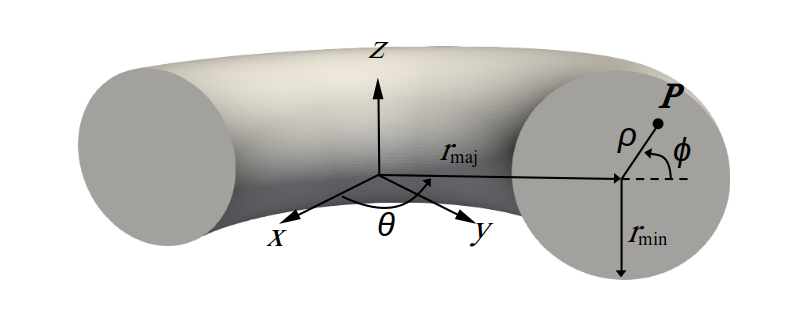
To validate our method and demonstrate its efficiency, we apply it to an idealized Hopfion structure, defined analytically by a set of equations and parameters. The following ansatz defines a Hopfion in an -torus of major radius and minor radius .
| (8) | ||||
| (9) | ||||
| (10) |
with
| (11) | ||||
| (12) | ||||
| (13) |
Here, defines the magnetization at the Hopfion’s core (), where , and at the torus surface (), where . Fig. 1 provides a schematic representation of the variables used in Eqs. (8)-(10).
Notably, while the inhomogeneous region of the magnetization is confined within the volume of the torus defined by and , the torus surface does not necessarily represent the physical boundary of the magnetic nanostructure. The magnetic texture described by this ansatz can be embedded into a homogeneous background magnetization in the direction with . In this case, the topological charge has compact support, meaning the topological features and the topological current are confined within the torus and vanish outside.
In Eqs. (8)-(10), the parameter introduces an additional phase for the in-plane magnetization components, allowing variation in the bimeron’s orientation across cross-sections. The parameters and are integer numbers determining the Hopfion’s chirality and order, with their values directly affecting the degree of winding, which is correlated with the Hopf index. Their impact on the vector field topology will be discussed below, in section VI. Setting , the magnetic configuration is axially symmetric, with each poloidal cross-section (along the meridional plane) exhibiting a bimeron structure, i.e., a vortex-antivortex pair with opposite core polarizationsGöbel et al. (2020).
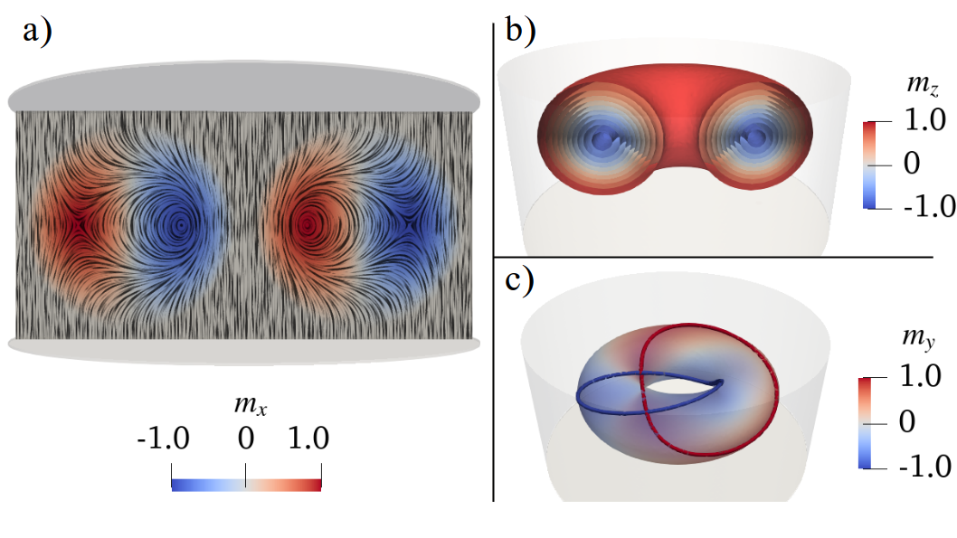
The characteristic toroidal isosurfaces composed of linked preimages displayed in Fig. 2 visually confirm that this analytic ansatz produces a magnetic texture with the defining features of a Hopfion.
V Numerical Results
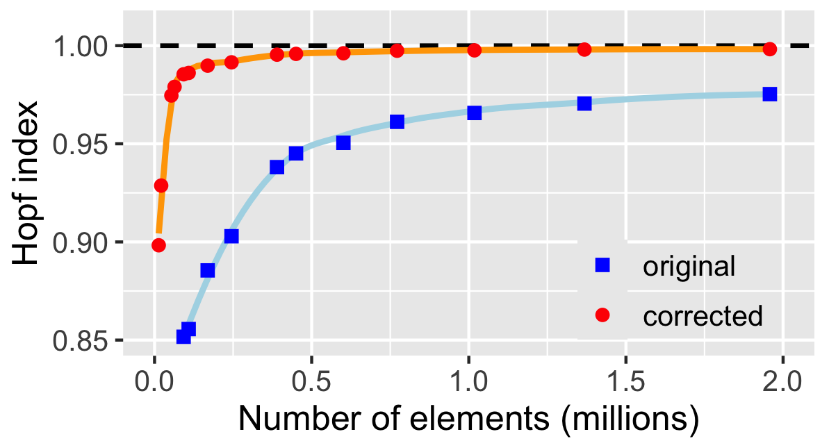
To test its correctness and accuracy, we apply the method described in section III and determine numerically the Hopf index of the analytically defined texture. With this model system, we expect to obtain a value close to unity in accordance with the topological characteristics of the Hopfion. Using Eqs. (8)-(10), we imprint the magnetic texture in a cylindrical geometry as illustrated in Fig. 2. The computed Hopf index is presented in Fig. 3 as a function of the number of finite elements used in the calculation.
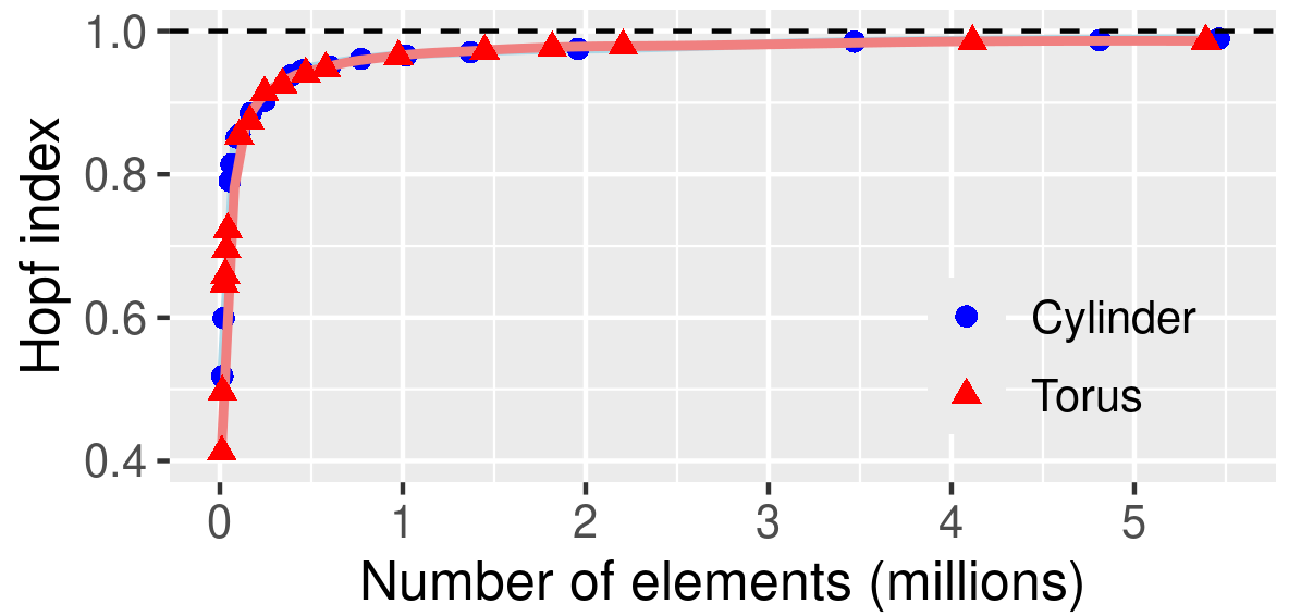
The ideal value is approached asymptotically as the number of elements increases. We observe this type of mesh-dependent convergence consistently across various shapes and geometries. For comparison, Fig. 3 also displays data for the analytic Hopfion defined in a torus geometry with and , demonstrating equivalent results for different sample shapes and confirming the method’s ability to handle arbitrarily shaped 3D geometries. In the remainder of this section, we focus exclusively on data for the cylinder geometry. While these results confirm the method’s overall correctness, they also highlight non-negligible numerical errors at low discretization levels and a sensitive dependence on the discretization density. A similar behavior was reported by Liu et al. Liu et al. (2018), despite using an entirely different numerical scheme. These numerical inaccuracies can be problematic in the case of strong inhomogeneities, where they may preclude the precise quantitative identification of a texture’s topological characteristics if the calculated Hopf index deviates too far from an integer value.
A primary source for the discretization errors is the numerical calculation of the topological current as defined in Eq. (3) since it involves several products of various spatial derivatives. Further numerical errors accumulate as is differentiated numerically on the right-hand side of the Poisson equation (5). In the context of the numerical analysis of the topological properties of Skyrmions, Kim et al. Kim and Mulkers (2020) introduced an elegant and efficient method to numerically determine the topological current with significantly higher accuracy by employing a lattice-based approach. In a recent article, Knapman et al.Knapman et al. (2025) demonstrated that this lattice-based method results in highly accurate numerical results for the case of Hopfions, too. The lattice-based approach, however, requires a coplanar distribution of discretization points—a criterion fulfilled in the case of finite-difference methods but inapplicable to finite-element methods, as discussed here, which use irregular discretization cells.
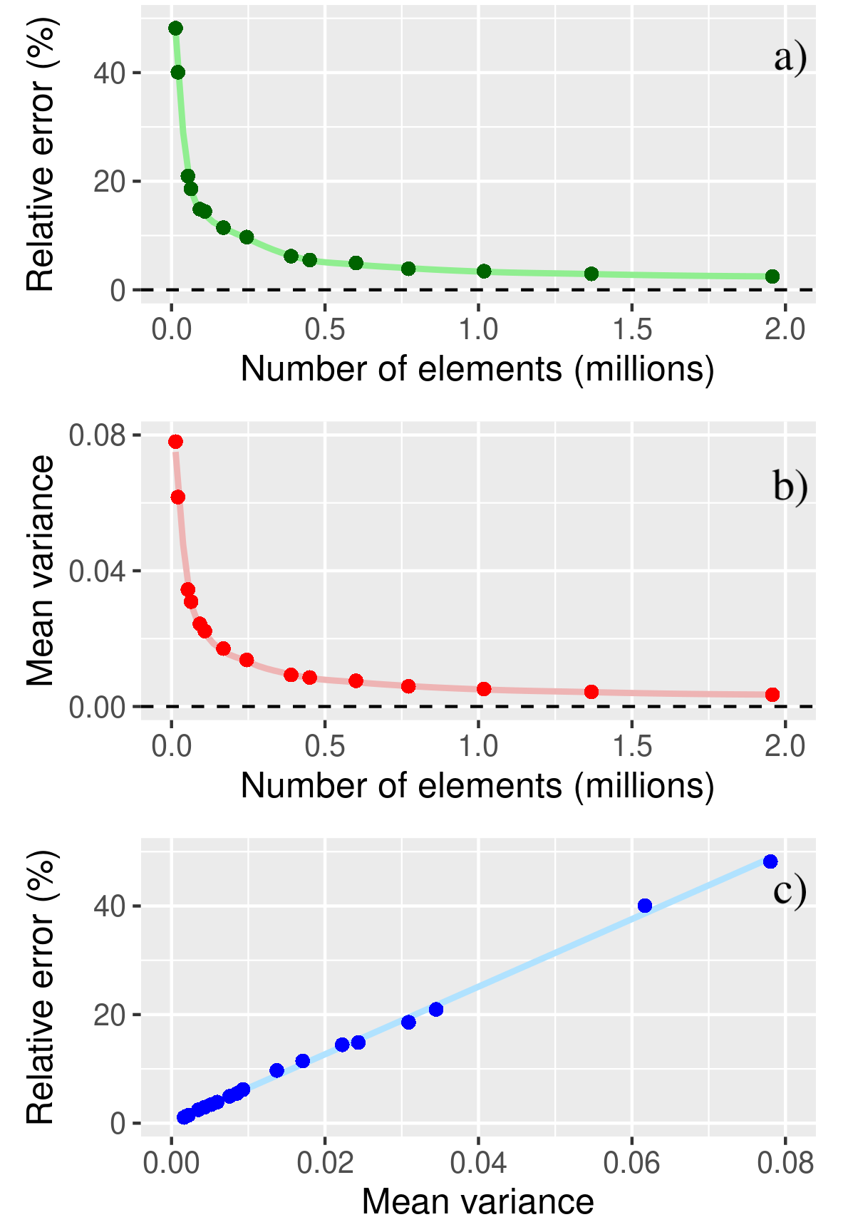
To improve the numerical accuracy of our FEM approach, we employ a phenomenological a posteriori error correction scheme. This scheme is based on two observations we made consistently by studying a wide variety of situations. Firstly, the effect of the error is to systematically underestimate the absolute value of the Hopf index. Such behavior is easier to correct than stochastic fluctuations of the computed values around the exact ones. Secondly, we observe a clear correlation between the size of the error and the variance of the magnetization, as shown in Fig. 4.
Here, the variance is defined element-wise and provides a measure of the misalignment of neighboring magnetic moments. For each tetrahedral element with its four nodes , we can define the variance through
| (14) | ||||
| (15) | ||||
| (16) |
where the brackets denote the mean of the values at the nodes of element . The value of ranges from zero in the case of a homogeneous state to one in the case of pairwise antiparallel alignment of the four magnetic moments. More generally, the value of the variance correlates with the angle enclosed between neighboring magnetic moments within a finite element—a quantity known to be tied to discretization errors in numerical micromagnetics Donahue (1998). It is therefore plausible to identify the variance as a measure or indicator for the occurrence of discretization errors. As shown in Fig. 4c), the relative error and the mean variance obtained for different meshes display a nearly linear dependence.
Based on these observations, i.e., the variance-dependent underestimation of the computed value, we design an error correction scheme to improve the calculated Hopf index . This is achieved through a function that yields a corrected value . However, the mean variance depends on the number of elements used in the simulation, including those in regions without topological texture, making it unsuitable for a generally applicable correction algorithm. Instead, we use the local variance , ascribed to each node through a volume-weighted average of the variance in the adjacent elements, to locate and quantify numerical errors. Our correction method augments the absolute value of the calculated Hopf density at each node by a factor that increases monotonically with the local variance. Despite the linear relationship between total error and mean variance illustrated in Fig. 4c), we did not achieve satisfactory results with a linear correction scheme based on the local variance. Rather than applying higher-order polynomial corrections, we improve the approximation by adopting a different functional form, where the Hopf density is increased at each node according to
| (17) |
with With this phenomenological approach, we obtain excellent results in a broad spectrum of situations by setting the constant’s value to .
Fig. 5 illustrates the impact of the correction scheme on the discretization-dependent values of the calculated Hopf index and the relative error. Near-perfect agreement with the expected analytic value is obtained already at moderate discretization levels, and we rapidly obtain a substantial reduction of the relative error. For instance, already at a moderate number of about finite elements, the corrected Hopf index is , very close to the expected value of , while the uncorrected index for the same mesh is . In this example, the correction decreases the relative error from to .
Despite the remarkable accuracy obtained with this method, we emphasize that our phenomenological a posteriori correction is not suitable to sizably reduce the local error in the calculation of the gradients or the topological current. This is because the local discretization error, unlike the Hopf index, does not increase monotonically with the variance. It is subject to fluctuations in both magnitude and sign that cannot be efficiently reduced with the same approach. However, the cumulative discretization errors affecting the integral (or, in numerical terms, the sum over the elements) in Eq. (1) can be significantly reduced in this manner.
We tested the method in several scenarios and geometries, considering different functional forms of the correction term and carefully tuning the constants involved. In all cases, the correction as described in Eq. (17) with yielded excellent results, leading us to the conclusion that the choice of the exponential correction function and the value of the constant are suitable for general cases, and are not specific to the texture discussed here. Eventually, we obtained enough confidence in this a posteriori correction to integrate it as a default operation into our algorithm to calculate the Hopf index. Hereafter, all reported Hopf index values are those corrected according to Eq. (17).
VI Higher-order Hopfions
The analytic formulation of Eqs. (8)-(10) enables the definition of higher-order Hopfion textures, e.i., with a Hopf index larger than one Rybakov et al. (2022), by selecting appropriate values for the parameters and . The parameter controls the number of bimerons in meridional cross-sections, as shown in Fig. 2a) for , while introduces a poloidal twist of the bimerons around the torus’ core circle (the spine) at . Figure (6) shows preimage representations of second-, third-, and fourth-order Hopfions in a torus geometry, obtained by setting and 4, respectively (with , and .
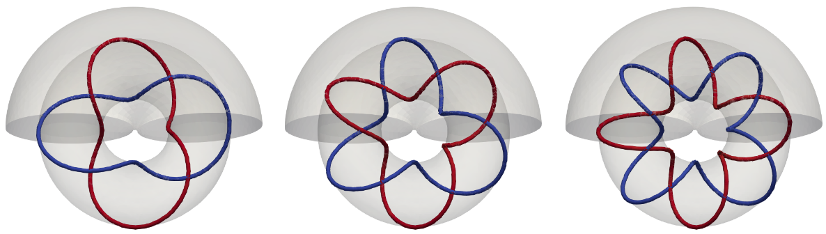
The poloidal twist generated by the parameter increases the vector field’s degree of topological knottedness, as evidenced by the increasingly complex linking of preimage lines. Accordingly, our method yields the Hopf indices 1.995, 2.998, and 3.999 for these structures, respectively, matching these textures’ ideal values 2, 3, and 4 very closely. These results further confirm our method’s ability to reliably and quantitatively characterize the topological properties of complex magnetization vector fields in arbitrary geometries.
VII Micromagnetic simulation
Having established the method’s reliability and accuracy using an idealized, analytically defined Hopfion texture, we now demonstrate an application example in a full-scale micromagnetic simulation. We consider a Hopfion bound in a cylindrical FeGe sample with height and radius . The material parameters are , , and , where is the ferromagnetic exchange constant, is the saturation magnetization, and is the bulk-type Dzyaloshinsky-Moria constant. To stabilize the Hopfion at zero fieldLiu et al. (2018), we apply a Néel-type surface anisotropy on the top and bottom surfaces of the cylinder, which pins the magnetization along the axis at the caps. We perform simulations using our custom-developed GPU-accelerated micromagnetic finite-element software tetmag Hertel (2023). To demonstrate the capacity of our method to reveal topological transitions, we investigate the quasistatic destruction of a Hopfion under an external magnetic field of increasing strength, monitoring field-induced changes in vector field topology through our method of calculating the Hopf index.
The simulation is initialized with a Hopfion inside the cylinder, defined by the ansatz of Eqs. (8)-(10) with , , , and , embedded into a homogeneous background magnetization . The numerical model employs a mesh with about 2 million irregularly shaped tetrahedral elements.
We perform quasi-static relaxation simulations with an external field applied along the positive -direction, varying from zero to in steps of . For each converged state, we calculate the Hopf index. The results are displayed in Fig. 7, where three different regions are apparent, which are separated by two discontinuous changes in the Hopf index—the first at and the second at .
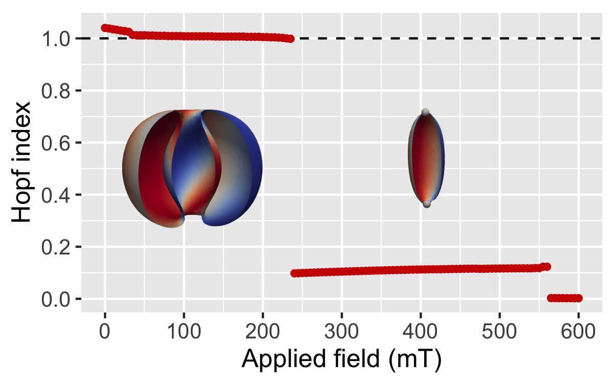
Between and , the Hopf index remains close to 1, consistent with the expected value given the presence of a Hopfion. At very low fields, the Hopf index exceeds this ideal value by up to about due to spurious effects related to weakly developed textures near the cylinder’s outer boundary, which are marginally connected to the Hopfion. The peripheral magnetization aligns more strongly with the applied field as the field increases beyond about (see Fig 8, a), causing these lateral textures to detach from the Hopfion, which becomes fully embedded into a homogeneous background magnetization . From to , the Hopf index stays nearly constant, with deviations below . Despite significant field-induced changes, in particular a reduction in the Hopfion’s size (Fig. 8), our correction method prevents any decrease in the Hopf index, even as local magnetic inhomogeneity increases. In this field range, where changes of the magnetization are reversible, the consistent Hopf index accurately reflects the topological equivalence of the textures, regardless of their field-induced deformation.
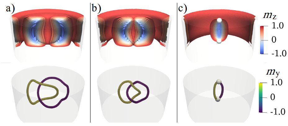
In the field range between and , the Hopf index remains almost constant at approximately 0.1; a significant decrease from its value in the first region. This abrupt reduction of the Hopf index at marks the irreversible destruction of the Hopfion, which transforms into a toron as Bloch points form on the top and bottom end of an encapsulated core region in which the magnetization is oriented along the negative axis, oppositely oriented to the surrounding background (Fig 8c). In the toron configuration, sometimes referred to as a coupled monopole-antimonopole pairLiu et al. (2018), the isosurfaces become homeomorphic to a sphere rather than a torus, and the previously closed, intertwined isolines in the preimage representation are now connected by two Bloch points. The change in vector field topology between the Hopfion and the toron configuration represents a topological transition that is characterized by an abrupt change in the Hopf index from 1 to 0.1. Like the first region, the Hopf index calculated in the toron regime remains constant over a wide range of field strengths, despite considerable field-induced modifications of the toron structure.
We emphasize that, while the change in the Hopf index indicates a topological change, the low value of 0.1 of the Hopf index does not allow definitive conclusions about the resulting magnetic structure beyond confirming the absence of a Hopfion. As discussed in section II, the Hopf index calculation relies on a smooth magnetization vector field and a divergence-free topological current. These conditions are not met in the vicinity of Bloch points, which represent sources and sinks of the topological currentLiu et al. (2018), invalidating the fundamental assumption required to introduce the vector potential according to Eq. (2). Consequently, the Helmholtz decomposition of the topological current becomes , where is a scalar potential accounting for the irrotational components. The vector potential captures only the solenoidal part of , which is insufficient for a full description of the Bloch point topology. The stable Hopf index of approximately 0.1 in the toron regime across a wide field range suggests that the divergence-free part of remains constant, potentially indicating a characteristic toron property. However, given the particular situation of a discontinuous magnetization vector field, we cannot rule out that spurious effects arising from the Bloch points may also contribute to the nonzero topological index. In any case, the fractional Hopf index calculated in this case cannot be interpreted topologically as a linking number.
In the third region, from to , except for a slight rotation on the lateral surface, the magnetization is overall homogeneous along the field direction, resulting in a vanishing Hopf index.
VIII Conclusion
We have developed a robust and accurate method for calculating the Hopf index in finite-element micromagnetic simulations. By employing the Biot-Savart form for the vector potential, our approach ensures gauge-invariant results even in multiply connected geometries. Applying our variance-based correction scheme to an analytically defined ideal Hopfion structure, we demonstrated its ability to significantly reduce numerical errors, which could otherwise be substantial in strongly inhomogeneous textures or exhibit slow mesh-size dependent convergence.
Through a micromagnetic simulation example involving a Hopfion’s field-induced destruction, we confirmed the method’s capacity to detect Hopfions and their absence, revealing topological transitions through abrupt changes in the Hopf index. Combined with the finite-element method’s flexibility in modeling magnetic textures in arbitrarily shaped 3D nanostructures, this approach enables precise identification and quantification of topological features in complex 3D magnetic configurations. Our method provides a powerful tool for advancing the study of topological magnetism in micromagnetic simulations. While we have only demonstrated its effectiveness in micromagnetism, we are confident that the method can also be applied successfully in other scientific domains, particularly in other ferroic material systems.
Acknowledgements
This work was supported by the French National Research Agency (ANR) under Contract No. ANR-22-CE92-0032 through the TOROID project co-funded by the Deutsche Forschungsgemeinschaft (DFG, German Research Foundation) Project No. 505561633 and by the France 2030 government investment plan managed by the French National Research Agency ANR under grant reference PEPR SPIN – [SPINTHEORY] ANR-22-EXSP-0009.
References
- Fernández-Pacheco et al. (2017) A. Fernández-Pacheco, R. Streubel, O. Fruchart, R. Hertel, P. Fischer, and R. P. Cowburn, Nature Communications 8, ncomms15756 (2017).
- Donnelly et al. (2017) C. Donnelly, M. Guizar-Sicairos, V. Scagnoli, S. Gliga, M. Holler, J. Raabe, and L. J. Heyderman, Nature 547, 328 (2017), number: 7663 Publisher: Nature Publishing Group.
- Bland and Heinrich (1995) J. Bland and B. Heinrich, eds., Ultrathin Magnetic Structures I, Vol. 1 (Springer-Verlag GmbH, Berlin, Heidelberg, New York, 1995) oCLC: 1081343538.
- Cheenikundil and Hertel (2021) R. Cheenikundil and R. Hertel, Applied Physics Letters 118, 212403 (2021), publisher: American Institute of Physics.
- Gołębiewski et al. (2024) M. Gołębiewski, R. Hertel, M. d’Aquino, V. Vasyuchka, M. Weiler, P. Pirro, M. Krawczyk, S. Fukami, H. Ohno, and J. Llandro, ACS Applied Materials & Interfaces 16, 22177 (2024), publisher: American Chemical Society.
- Fischer et al. (2020) P. Fischer, D. Sanz-Hernández, R. Streubel, and A. Fernández-Pacheco, APL Materials 8, 010701 (2020), number: 1 Publisher: American Institute of Physics.
- Birch et al. (2020) M. T. Birch, D. Cortés-Ortuño, L. A. Turnbull, M. N. Wilson, F. Groß, N. Träger, A. Laurenson, N. Bukin, S. H. Moody, M. Weigand, G. Schütz, H. Popescu, R. Fan, P. Steadman, J. a. T. Verezhak, G. Balakrishnan, J. C. Loudon, A. C. Twitchett-Harrison, O. Hovorka, H. Fangohr, F. Y. Ogrin, J. Gräfe, and P. D. Hatton, Nature Communications 11, 1726 (2020), number: 1 Publisher: Nature Publishing Group.
- Milde et al. (2013) P. Milde, D. Köhler, J. Seidel, L. M. Eng, A. Bauer, A. Chacon, J. Kindervater, S. Mühlbauer, C. Pfleiderer, S. Buhrandt, C. Schütte, and A. Rosch, Science 340, 1076 (2013), number: 6136.
- Leonov and Inoue (2018) A. O. Leonov and K. Inoue, Physical Review B 98, 054404 (2018), publisher: American Physical Society.
- Zheng et al. (2018) F. Zheng, F. N. Rybakov, A. B. Borisov, D. Song, S. Wang, Z.-A. Li, H. Du, N. S. Kiselev, J. Caron, A. Kovács, M. Tian, Y. Zhang, S. Blügel, and R. E. Dunin-Borkowski, Nature Nanotechnology 13, 451 (2018), number: 6 Publisher: Nature Publishing Group.
- Kent et al. (2021) N. Kent, N. Reynolds, D. Raftrey, I. T. G. Campbell, S. Virasawmy, S. Dhuey, R. V. Chopdekar, A. Hierro-Rodriguez, A. Sorrentino, E. Pereiro, S. Ferrer, F. Hellman, P. Sutcliffe, and P. Fischer, Nature Communications 12, 1562 (2021), number: 1 Publisher: Nature Publishing Group.
- Rybakov et al. (2022) F. N. Rybakov, N. S. Kiselev, A. B. Borisov, L. Döring, C. Melcher, and S. Blügel, APL Materials 10, 111113 (2022), publisher: American Institute of Physics.
- Zheng et al. (2023) F. Zheng, N. S. Kiselev, F. N. Rybakov, L. Yang, W. Shi, S. Blügel, and R. E. Dunin-Borkowski, Nature 623, 718 (2023), publisher: Nature Publishing Group.
- Göbel et al. (2020) B. Göbel, C. A. Akosa, G. Tatara, and I. Mertig, Physical Review Research 2, 013315 (2020), publisher: American Physical Society.
- García-Cervera et al. (2003) C. J. García-Cervera, Z. Gimbutas, and W. E, Journal of Computational Physics 184, 37 (2003), number: 1.
- Whitehead (1947) J. H. C. Whitehead, Proceedings of the National Academy of Sciences 33, 117 (1947).
- Faddeev and Niemi (1997) L. Faddeev and A. J. Niemi, Nature 387, 58 (1997), publisher: Nature Publishing Group.
- Wilczek and Zee (1983) F. Wilczek and A. Zee, Physical Review Letters 51, 2250 (1983), number: 25 Publisher: American Physical Society.
- Nicole (1978) D. A. Nicole, Journal of Physics G: Nuclear Physics 4, 1363 (1978).
- Liu et al. (2018) Y. Liu, R. K. Lake, and J. Zang, Physical Review B 98, 174437 (2018), number: 17 Publisher: American Physical Society.
- Tai and Smalyukh (2018) J.-S. B. Tai and I. I. Smalyukh, Physical Review Letters 121, 187201 (2018), publisher: American Physical Society.
- Komineas and Papanicolaou (1996) S. Komineas and N. Papanicolaou, Physica D: Nonlinear Phenomena 99, 81 (1996).
- Thiele (1973) A. A. Thiele, Physical Review Letters 30, 230 (1973), number: 6.
- Han (2017) J. H. Han, Skyrmions in Condensed Matter, Springer Tracts in Modern Physics, Vol. 278 (Springer International Publishing, Cham, 2017).
- Note (1) The property is central to this formalism, as it allows to introduce a vector potential according to eq. (2). This condition of a solenoidal field is not fulfilled in the case of Bloch points, where the magnetization’s spatial gradients are undefined.
- Arnold and Khesin (2021) V. I. Arnold and B. A. Khesin, Topological Methods in Hydrodynamics, Applied Mathematical Sciences, Vol. 125 (Springer International Publishing, Cham, 2021).
- Ackerman and Smalyukh (2017) P. J. Ackerman and I. I. Smalyukh, Physical Review X 7, 011006 (2017), publisher: American Physical Society.
- Smalyukh (2020) I. I. Smalyukh, Reports on Progress in Physics 83, 106601 (2020), number: 10 Publisher: IOP Publishing.
- Sutcliffe (2017) P. Sutcliffe, Physical Review Letters 118, 247203 (2017), publisher: American Physical Society.
- Luk’yanchuk et al. (2020) I. Luk’yanchuk, Y. Tikhonov, A. Razumnaya, and V. M. Vinokur, Nature Communications 11, 2433 (2020).
- Ricca and Liu (2024) R. L. Ricca and X. Liu, eds., Knotted Fields, Lecture Notes in Mathematics, Vol. 2344 (Springer Nature Switzerland, Cham, 2024).
- Moffatt (1969) H. K. Moffatt, Journal of Fluid Mechanics 35, 117 (1969).
- Moreau (1961) J.-J. Moreau, Comptes rendus hebdomadaires des séances de l’Académie des sciences 252, 2810 (1961).
- Dennis et al. (2010) M. R. Dennis, R. P. King, B. Jack, K. O’Holleran, and M. J. Padgett, Nature Physics 6 (2010), 10.1038/nphys1504, publisher: Nature Publishing Group.
- Barnett et al. (2023) S. M. Barnett, F. C. Speirits, and J. B. Götte, Europhysics Letters 143, 35002 (2023), publisher: EDP Sciences, IOP Publishing and Società Italiana di Fisica.
- Rajaraman (1982) R. Rajaraman, Solitons and Instantons: An Introduction to Solitons and Instantons in Quantum Field Theory (Amsterdam: North-Holland, 1982).
- Arafune et al. (1975) J. Arafune, P. G. O. Freund, and C. J. Goebel, Journal of Mathematical Physics 16, 433 (1975).
- Berger and Field (1984) M. A. Berger and G. B. Field, Journal of Fluid Mechanics 147, 133 (1984).
- Woltjer (1958) L. Woltjer, Proceedings of the National Academy of Sciences 44, 489 (1958), publisher: Proceedings of the National Academy of Sciences.
- MacTaggart and Valli (2019) D. MacTaggart and A. Valli, Journal of Plasma Physics 85, 775850501 (2019).
- Bevir and Gray (1980) M. Bevir and J. W. Gray, Proceedings of the Reversed-Field Pinch Theory Workshop LA-8944-C, 176 (1980).
- Hertel and Kákay (2014) R. Hertel and A. Kákay, Journal of Magnetism and Magnetic Materials 369, 189 (2014).
- Fredkin and Koehler (1990) D. R. Fredkin and T. R. Koehler, IEEE Transactions on Magnetics 26, 415 (1990), number: 2.
- Demidov (2019) D. Demidov, Lobachevskii Journal of Mathematics 40, 535 (2019), number: 5.
- Kim and Mulkers (2020) J.-V. Kim and J. Mulkers, IOP SciNotes 1, 025211 (2020), number: 2 Publisher: IOP Publishing.
- Knapman et al. (2025) R. Knapman, M. Azhar, A. Pignedoli, L. Gallard, R. Hertel, J. Leliaert, and K. Everschor-Sitte, Physical Review B 111, 134408 (2025), publisher: American Physical Society.
- Donahue (1998) M. J. Donahue, Journal of Applied Physics 83, 6491 (1998), number: 11.
- Hertel (2023) R. Hertel, “tetmag,” https://github.com/R-Hertel/tetmag (2023).