scale=1, angle=0, opacity=1, color=black, contents=

See pages - of figure/Manuscript_vf.pdf

Supplementary Information: Wavefront Shaping of Scattering Forces Enhances Optical Trapping of Levitated Nanoparticles

1 Experimental setup

1.1 Optical trap

Figure S1 provides a schematic description of the experimental setup. A linearly polarized 1064 nm continuous laser (AzurLight System, 10 W) delivers roughly $\sim$300 mW of power at the input of a vacuum chamber. Inside the chamber, the beam is focused using a high-numerical-aperture objective (Olympus LMPlan IRx100, NA = 0.8, WD = 3.4 mm), forming a single-beam gradient optical trap, while an aspheric lens (NA = 0.55) collects the transmitted light. The particles used in the experiment consist of silica nanobeads with radii of 75, 100, 110, and 125 nm (density: $\rho$ = 2200 kg.m^-3, refractive index: n = 1.45), sourced from Microparticles GmbH and NanoCym. Before trapping, they undergo a preheating process at 600°C for 3 hours. This treatment stabilizes the particles by eliminating Si-OH surface groups and forming durable Si-O-Si bonds[1]. A suspension of these particles in isopropanol is then sprayed into the chamber at atmospheric pressure using an Omron Micro-Air nebulizer.

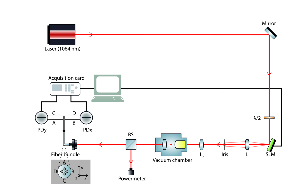
Figure S1: Schematic representation of the experimental setup. The optical phase of a 1064 nm continuous laser beam is spatially shaped by an spatial light modulator (SLM) before being focused into a vacuum chamber using a high-numerical-aperture objective, thus forming an optical trap. The beam is then recollected and analyzed using a differential photodiode system to extract motional power spectral densities (PSDs).

The center-of-mass (COM) motion of the trapped particle is detected via spatial integration of the interference pattern formed between the trapping and scattered fields. As illustrated in Fig. S1, a split detection scheme, sensitive to transverse motion, is implemented by spatially dividing the beam using a 1-to-4 multimode fiber bundle, with each fiber being coupled to a differential photodiode. Motion along the optical axis can be measured on both photodiodes. COM displacements are recorded simultaneously along all three directions using a DAQ operating at a sampling rate of 5 MS/s and acquiring 20-second long time traces. Figure S2 provides an example of measured power spectral densities (PSDs) along all three axes under a uniform wavefront (i.e., no modulation on the SLM).

Figure S2: Mechanical spectra measured in the absence of SLM modulation. PSDs along all three axes for a 125 nm particle, at 1 mbar, trapped using a uniform wavefront and an optical power of $\approx 300mW$ at the input of the vacuum chamber.

1.2 Wavefront shaping

We use a phase-only Spatial Light Modulator (SLM, Holoeye PLUTO-2.1 NIR149) with a resolution of 1920×1080 pixels and an 8 µm pixel pitch. The SLM modulates the phase of the beam before it passes through the trapping objective. Due to the Fourier transform relationship between the field at the SLM plane and the field at the focal plane of the objective, the phase-only modulation applied to the beam upstream translates (directly) into intensity modulations at the trap’s location. To fully exploit the capabilities of the SLM, it is initially configured into a blazed diffraction grating. If this grating splits the beam into multiple diffraction orders, it reflects about $\approx 60\%$ of the incoming light intensity into the first order. Additional phase modulation patterns (of lower spatial frequencies) are then superimposed onto this blaze grating. According to Fourier optics, this superposition in the phase domain corresponds to a convolution of the patterns after the trapping objective, allowing the nonzero diffraction orders to be modulated. An iris is used to isolate the first diffraction order, which carries the desired phase-modulated beam, while eliminating the zero-order as well as higher-order contributions.

To determine the position of the incident beam on the SLM, we use a masking technique combined with the diffraction grating pattern. The blaze grating pattern is applied only within a circular aperture; elsewhere, the phase modulation is set to zero (constant phase). The radius of this circular mask is chosen to be smaller than the size of the incident beam. The center of the circular mask is moved across the SLM surface in steps of 4 pixels. For each position of the mask, we measure the power of the first diffraction order after the trapping objective. The recorded power indicates the overlap between the incident beam and the modulated region of the SLM. By scanning the mask position, we pinpoint the spatial location of the beam’s center on the SLM.

1.3 Stiffness optimization

The phase patterns or wavefronts used for stiffness optimization are constructed as linear combinations of Zernike polynomials. As illustrated in Fig. S5, we use a basis made of 30 polynomials, whose first 20 elements are axis-symmetric ($Z_{i}^{0}$) while the remaining 10 are not ($Z_{i}^{k\neq 0}$). Zernike polynomials are particularly well-suited for wavefront shaping due to their orthogonality and their ability to accurately represent a wide range of optical aberrations.

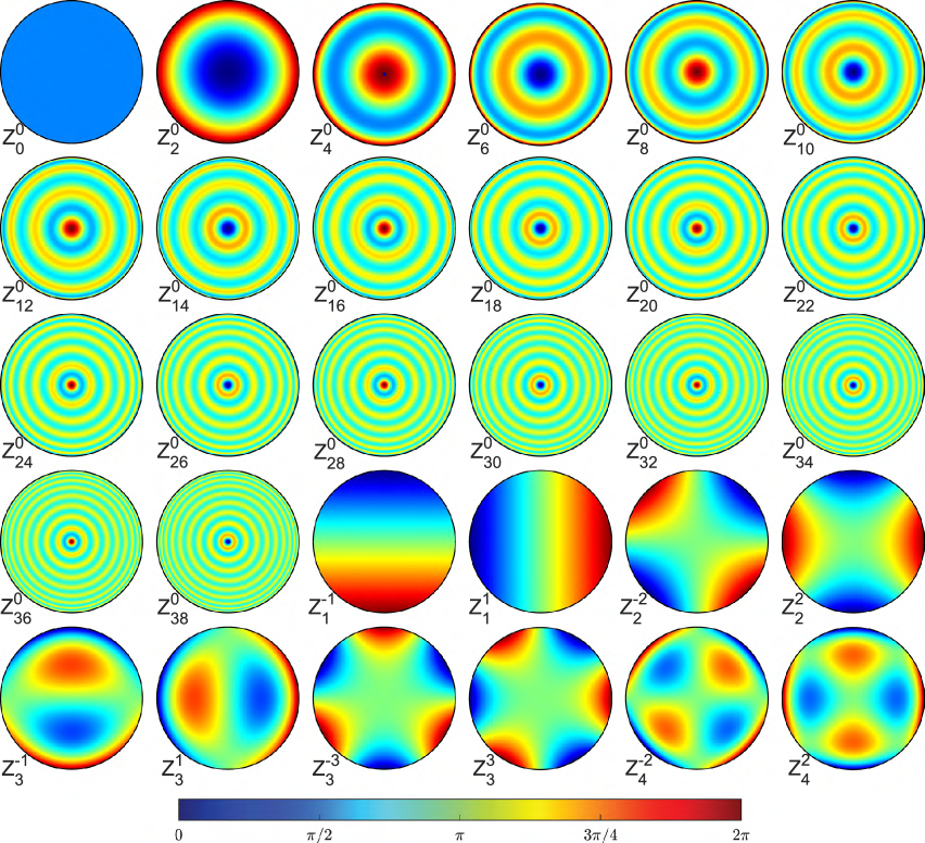
Figure S5: Wavefront-shaping expansion basis. Zernike polynomials used for the optimization protocol.

In order to optimize the stiffness, we employ a gradient-free algorithm (fminsearch, Matlab). This iterative algorithm adjusts the contribution of each Zernike polynomial to maximize a given cost function without requiring gradient calculations, which are known to be extremely sensitive to experimental noise. By avoiding abrupt phase changes, this approach also ensures smooth wavefront adjustments, thus reducing the risk of particle loss throughout the process. For each iteration, an initial acquisition is performed using the uniform (i.e., unmodulated) beam to measure the baseline resonance frequencies, followed by a second acquisition with the applied phase pattern. Here, we recall that the resonance frequency $f_{i\in\{x,y,z\}}$ along each axis is related to the trap stiffness $\kappa_{i\in\{x,y,z\}}$ and the particle’s mass $m$ through the relationship

$$2\pi f_{i}=\sqrt{\frac{\kappa_{i}}{m}}$$ (1)

We then estimate a cost function of the form

$$f(X)=\alpha(f_{opt,x}/f_{0,x})^{2}+\beta(f_{opt,y}/f_{0,y})^{2}+\gamma(f_{opt,z}/f_{0,z})^{2}$$ (2)

, where $f_{0,i}$ and $f_{opt,i}$ represent respectively the resonance frequencies of the uniform and optimized traps, while the terms $\alpha$, $\beta$ and $\gamma$ stand for adjustable coefficients and $X$ denotes the wavefront (i.e., linear combination of Zernike polynomials used to generate the wavefront). The coefficients $\alpha$, $\beta$ and $\gamma$ can be adjusted to improve the optimization of one direction over the others. This cost function is motivated by the proportionality between stiffness and the square of the resonance frequency as well as the fact that measuring the uniform resonance frequency at each iteration mitigates the impact of power drifts (thus ensuring an accurate evaluation of relative stiffness improvements).

1.4 Experimental results

Figure S6 illustrates the evolution of the relative stiffness during three optimization routines performed on a particle of 110 nm in radius using three different cost functions.

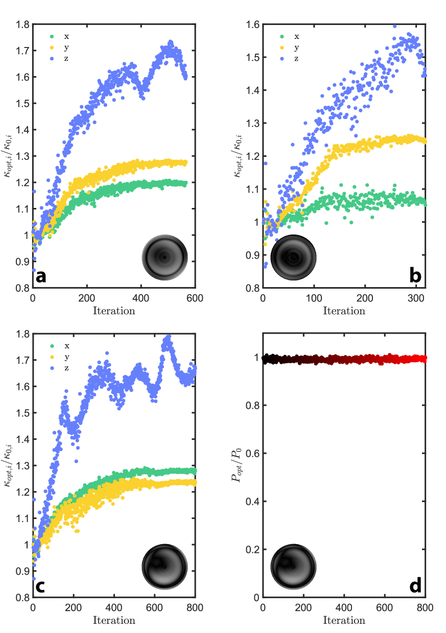
Figure S6: Different examples of experimental optimizations. a, b, c- Evolution of the relative stiffness along each axis (see legend and color scheme) throughout the optimization for three different cost functions. d- Evolution of the optical power, $P_{opt}$, at each iteration throughout the optimization displayed in c. The power is measured by a photodiode positioned after the vacuum chamber and normalized by the value collected for a uniform wavefront, $P_{0}$.

The first cost function (Fig. S6a), optimizes the relative stiffness along all three directions and reads

$$f(X)=(f_{opt,x}/f_{0,x})^{2}+(f_{opt,y}/f_{0,y})^{2}+\frac{1}{2}(f_{opt,z}/f_{0,z})^{2}$$

This results in relative stiffness ratios $\kappa_{opt,x}/\kappa_{0,x}=1.19$, $\kappa_{opt,y}/\kappa_{0,y}=1.26$ and $\kappa_{opt,z}/\kappa_{0,z}=1.73$. Here, the coefficient $\gamma=1/2$ is introduced to mitigate optimization difficulties due to measurement uncertainties along $z$. This cost function corresponds to the one used in Figure 1 of the main text in the case of 125-nm levitated particles.

The second optimization (Fig. S6b) focuses solely on maximizing the stiffness along the $y$-axis, using the cost function

$$f(X)=(f_{opt,y}/f_{0,y})^{2}$$

While this also enhances stiffness along $z$, it has a negligible effect on $x$ and the corresponding stiffness ratios are respectively $\kappa_{opt,x}/\kappa_{0,x}=1.08$, $\kappa_{opt,y}/\kappa_{0,y}=1.26$ and $\kappa_{opt,z}/\kappa_{0,z}=1.57$.

Finally, the third optimization (Fig. S6c) targets the $x$-axis specifically, using the cost function-

$$f(X)=(f_{opt,x}/f_{0,x})^{2}$$

This approach leads to the highest relative stiffness along $x$, making it the only case where $\kappa_{x}>\kappa_{y}$, yielding ratios $\kappa_{opt,x}/\kappa_{0,x}=1.29$, $\kappa_{opt,y}/\kappa_{0,y}=1.24$ and $\kappa_{opt,z}/\kappa_{0,z}=1.79$.

The three resulting wavefronts, shown in Fig. S6, exhibit distinct differences, demonstrating the impact of the choice of the cost function on the optimized wavefront. Furthermore, Fig. S6d shows the evolution of the relative power measured by a photodiode located after the vacuum chamber (see Fig. S1) throughout the third optimization routine. The constant power level confirms that the optimization process does not affect the alignment of the beam or the filling factor of the trapping objective.

Figure S3: Uniform vs optimized spectra. a, b and c- PSDs for the uniform (black) and optimized (red) wavefront, which are measured along the $x$, $y$ and $z$-axis, respectively. d- Relative contributions of the different Zernike polynomials to the optimized wavefront used in a, b and c (see Fig. S5).

To provide insights into how the wavefront is reshaped, Fig. S3 focuses on the optimization routine being applied to a nanoparticle with a 125 nm radius (which does not correspond to the one used in the main text). The Figs. S3a-c provide the PSDs for each axis measured before (’Uniform’, black) and after (’Optimized’, red) the optimization. Figure S3d displays the relative distribution of the different Zernike polynomials (Fig. S5) that compose the optimized wavefront. It can be observed that the axis-symmetric polynomials (i.e., $Z_{i}^{0}$ with $i\in[0,38]$) of lower rank seem to be more involved.

At last, the robustness of the optimized-wavefront solution is further explored in Fig. S4. This figure shows the relative stiffness enhancement for particles of different sizes using the optimized pattern obtained in Figure 1 of the main article. These results indicate that a pattern optimized for a given size remains effective for particles of different radii. Nonetheless, the optimization is less efficient than when performed directly on the particle of the proper dimension.

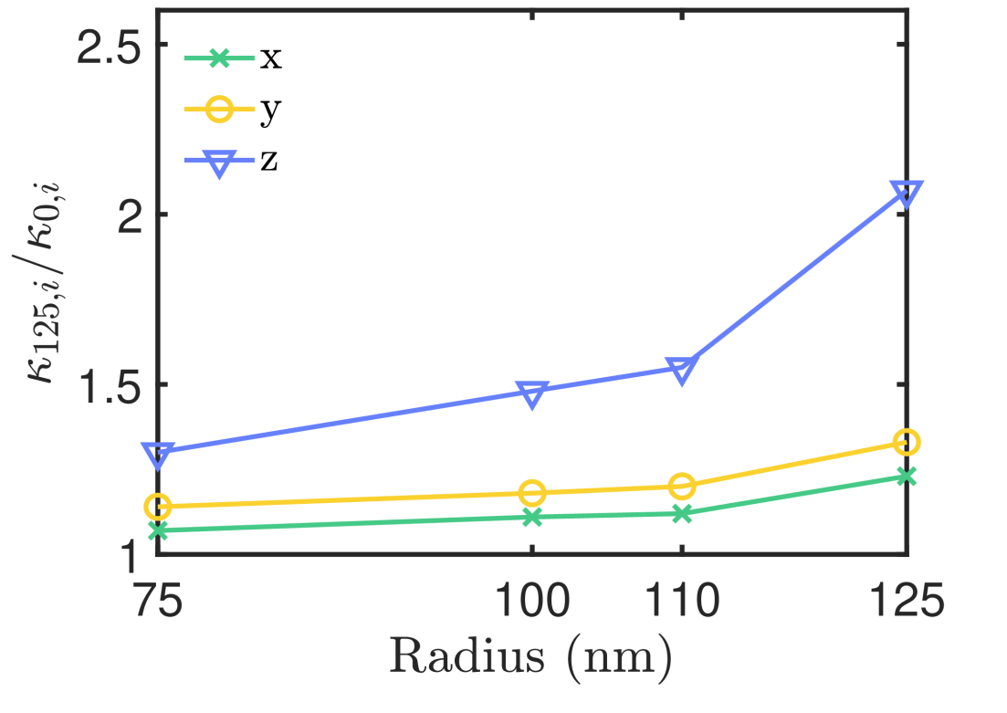
Figure S4: Stiffness enhancement ratios obtained for different radii when applying the wavefront from Figure 1 of the main text. Relative stiffness for each axis as a function of the particle’s size, using the pattern from the main text. The notation $\kappa_{125}$ indicates that the wavefront was optimized for a particle of 125 nm in radius.

2 Numerical simulations of the optimization process

2.1 Forces computation and multipole expansion

To model the trapping field for various numerical apertures, NA, filling factors, $f_{0}$, and wavefronts, $X$, we use a modified Debye integral. Specifically, we include a thin-lens apodization function (see equation (3.56) of Ref [2]), which accounts for the SLM-modulated wavefront. The field scattered by the particle is expressed using the Generalized Lorentz Mie Theory (GLMT), which ultimately enables to compute ’exactly’ the optical forces using the Maxwell Stress Tensor (MST) [3]. This method is used to benchmark a much faster semi-analytical method, which provides the total force as a sum of different multipole contributions [4, 5].

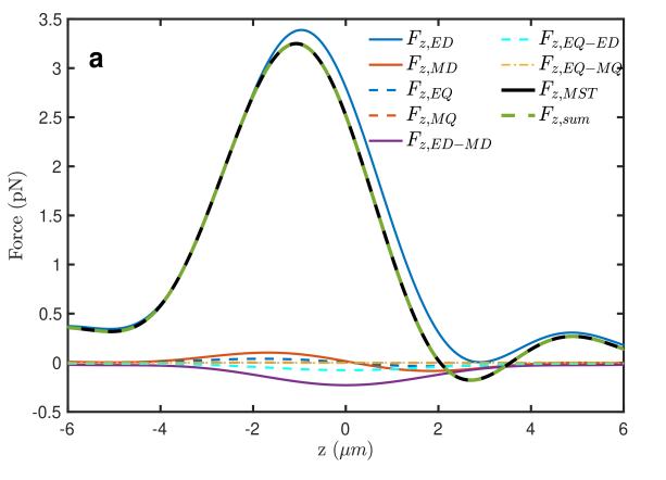
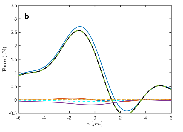
Figure S7: Simulations of axial-force landscapes. a- Landscape of the axial force, $F_{z}$, for a uniform wavefront. The black curve represents the ’exact’ MST computation, $F_{z,MST}$. The other curves (see legend and text) describe the different multipole contributions. When adding up all these contributions, we obtain a total force (dashed green, $F_{z,sum}$) identical to the one computed using the MST. b- Similar force landscape to that in a but here for an optimized wavefront (same legend and color code). c and d show magnified views of a and b around their corresponding trapping points, respectively.

The optimization routine is performed by computing, at each iteration, the force landscapes along $x$, $y$ and $z$, labeled $F_{x}(x)$, $F_{y}(y)$ and $F_{z}(z)$, respectively. Such computations are achieved using the multipole method (introduced above) up to the quadrupole order. The modulated wavefront is reproduced by decomposing the apodization function into $32$ to $128$ concentric rings with different optical phases. The distribution of the phase on each ring emulates a wavefront $X$, which is iteratively optimized to maximize a cost function similar to the one provided in section 1.3. Varying the number of rings, as well as the starting guess, we observe a convergence towards wavefronts similar to the ones obtained experimentally. Figure S7 shows in black the axial-force landscape, $F_{z,MST}(z)$, computed for a uniform (panel a) and an optimized wavefront (panel b), which display a gain in axial stiffness $\kappa_{z}$ close to a factor of 2.2 (see Figure 2 of the main text). Zoomed-in views of both landscapes are provided in Figs. S7a and d. Here, the simulation parameters are set to an NA=$0.68$ and a filling factor $f_{0}=0.7$, for a particle of radius 125 nm trapped using a beam power of 350 mW. We underline, however, that a stiffness gain higher than 2 (as discussed in this work) has been observed numerically for a wide range of particle radii, numerical apertures and filling factors. We also note that the coordinate $z$ in the optimized case has been shifted such that the conservative part of the force (i.e., gradient force, see section 2.2) remains zero at $z=0$ (i.e., the beam focus).

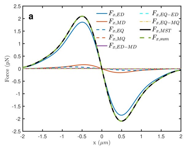
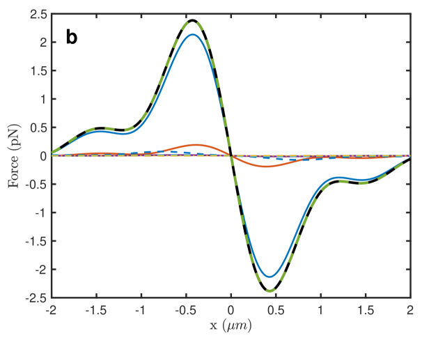
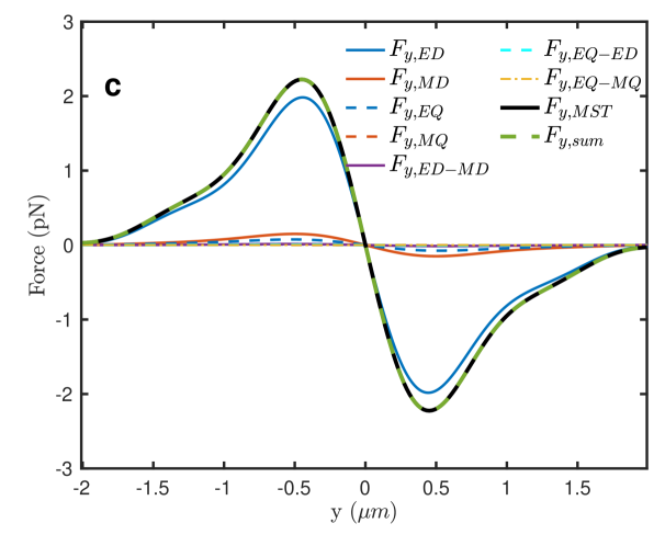
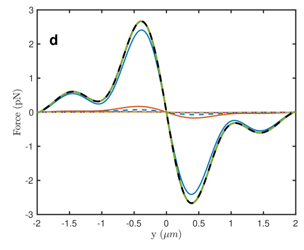
Figure S9: Simulations of transverse-force landscapes. a, b- Force landscapes $F_{x}$ computed using the two approaches introduced in Fig. S7 and for the same wavefronts (respectively uniform in a and optimized in b). c, d- Force landscapes $F_{y}$ computed using the two approaches introduced in Fig. S7 and for the same wavefronts (respectively uniform in c and optimized in d).

In Figs. S7a and b, the different multipole contributions provided by our numerical method are displayed. In particular, we plot the force originating from the electric dipole (ED, blue), the magnetic dipole (MD, red), the electric quadrupole (EQ, dashed blue) and the magnetic quadrupole (MQ, dashed red). There, we also report the force produced by the interferences between the electric and magnetic dipoles (ED-MD, purple), between the electric dipole and quadrupole (ED-EQ, dashed light blue) as well as between the electric and magnetic quadrupoles (EQ-MQ, dot-dashed yellow) [4]. The curve in dashed green shows the sum of these different multipole contributions, which matches the ’exact’ computation performed using the Maxwell Stress Tensor (black). In Figs. 2a and b of the main text, the interference terms have been added to the magnetic dipole and electric quadrupole contributions to make these figures easier to understand. As expected for such a small nanoparticle, these simulations clearly emphasize that the electric dipole is the dominant contribution to the total force along the $z$-axis. They also show that the optimization mainly acts on the electric-dipole term, while other contributions remain largely unaffected. In other words, the optimization primarily reshapes the electric-dipole contribution in order to increase the stiffness.

For the optimization displayed in Figure 2 of the main text and reproduced in Fig. S7, Fig. S9 shows in black the exact calculations of the forces along the two transverse directions, respectively $F_{x,MST}$ and $F_{y,MST}$. We also provide the multipole expansion of the forces using the same color code and naming scheme as in Fig. S7. Similarly to the axial direction, we observe that the optimization mainly acts on the dominant electric dipole to improve the stiffness along the transverse directions. As sketched in Figure 2c of the main text, the optimization brings the particle closer to the focus, where the intensity gradient is stiffer in the transverse plane, which readily improves the optical confinement.

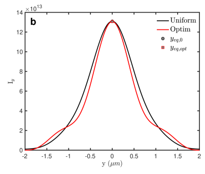
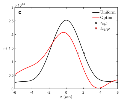
Figure S8: Uniform and optimized local intensities close to the equilibrium positions. a, b and c- Intensity profiles $I_{x}$, $I_{y}$ and $I_{z}$ (in arbitrary units), which are computed respectively along $x$, $y$ and $z$ for the uniform (red) and optimized (black) wavefronts of Figs. S7 and S9, respectively. The black squares and red dots pinpoint the equilibrium locations along each axis.

After optimization, the optical trap becomes more photon-efficient, in that it can produce the same stiffness as in the uniform case but with significantly less incoming laser intensity. This point is confirmed in Fig. S8, which plots along the three directions $x$, $y$ and $z$ the field intensities in the vicinity of the focal spot for the uniform (black) and optimized (red) wavefronts. We readily observe that the intensity at the equilibrium position remains similar in both cases (black squares and red dots for uniform and optimized $z_{eq}$, respectively). Thus, as the stiffness is more than doubled by the optimized wavefront (multiplied by $\approx 2.2$), one can achieve the same stiffness as in the uniform case with an incoming laser power reduced by more than $50\%$ (i.e., divided by a factor of 2.2).

2.2 Conservative and non-conservative parts

The multipole expansion performed in Figs. S7 and S9, can be harnessed to decompose analytically the different terms into their non-conservative (i.e., scattering) and conservative (i.e., gradient) parts [6]. Since this decomposition is only provided along $z$ in Fig. 2d of the main text, we only consider the axial forces below. In particular, the conservative and non-conservative parts are labeled respectively $F_{g,j}$ and $F_{s,j}$, with $j$ indicating the multipole considered.

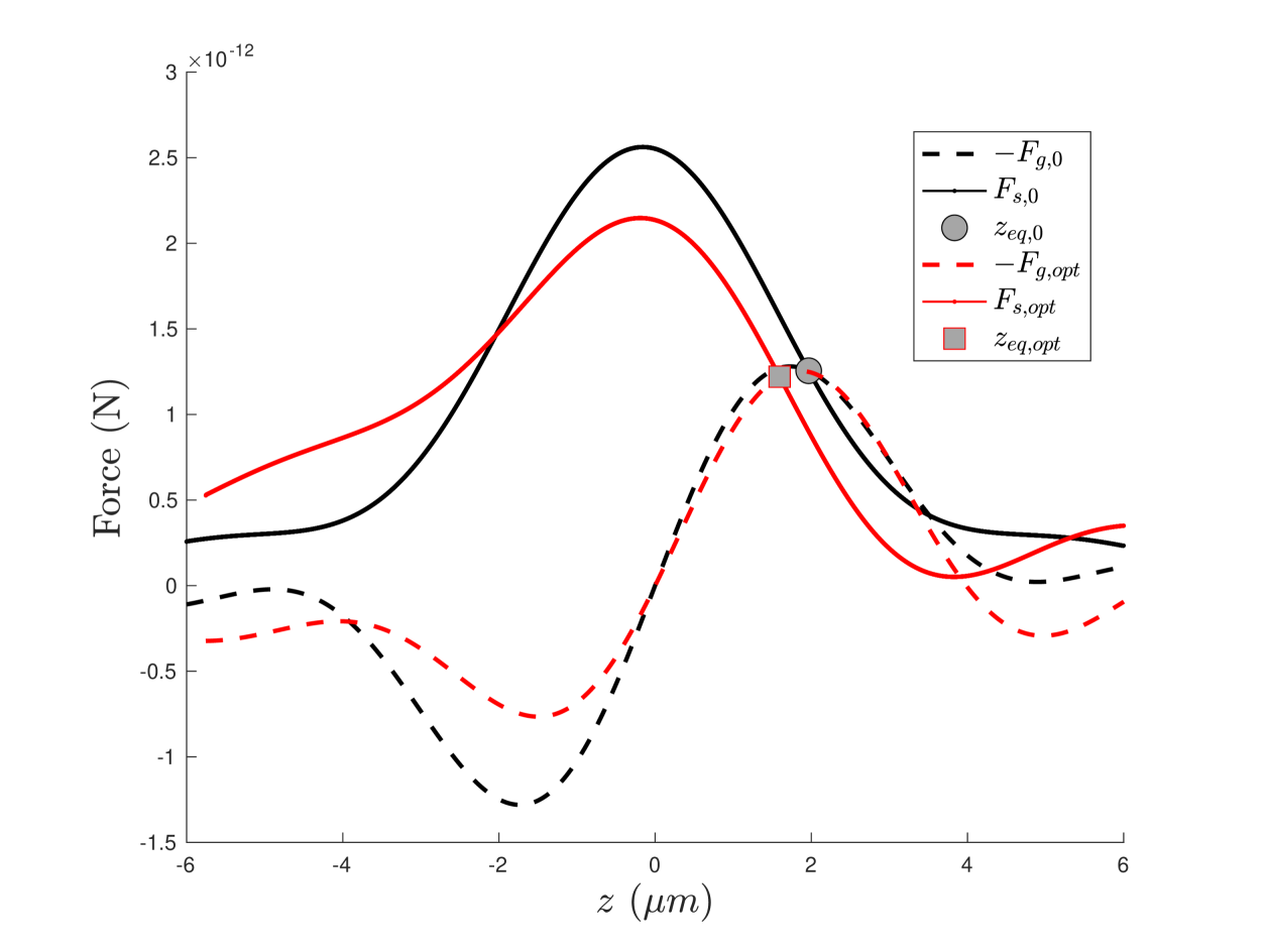
Figure S10: Conservative and non-conservative contributions to the axial force. The total axial force, $F_{z}$, is decomposed into its conservative and non-conservative parts, see Eqs. (3, 4). For the uniform wavefront, we plot in black $-F_{g,0}$ and $F_{s,0}$, which intersect at the equilibrium position $z_{eq,0}$. For the optimized wavefront, we plot in red $-F_{g,opt}$ and $F_{s,opt}$, which intersect at the equilibrium position $z_{eq,opt}$.

For the conservative parts:

$$F_{g,{ED}} = \frac{\varepsilon_{0}}{2}\rm{Re}\left(\alpha_{ED}\right).\rm{Re}\left(\frac{\partial E_{j}}{\partial z}E_{j}^{\star}\right)$$ (3)

$$F_{g,{MD}} = \eta_{0}^{2}\frac{\varepsilon_{0}}{2}\rm{Re}\left(\alpha_{MD}\right).\rm{Re}\left(\frac{\partial H_{j}}{\partial z}H_{j}^{\star}\right)$$

while, for the non-conservative parts:

$$F_{s,{ED}} = \frac{\varepsilon_{0}}{2}\rm{Im}\left(\alpha_{ED}\right).\rm{Im}\left(\frac{\partial E_{j}}{\partial z}E_{j}^{\star}\right)$$ (4)

$$F_{s,{MD}} = \eta_{0}^{2}\frac{\varepsilon_{0}}{2}\rm{Im}\left(\alpha_{MD}\right).\rm{Im}\left(\frac{\partial H_{j}}{\partial z}H_{j}^{\star}\right)$$

$${F_{s,ED-MD}} = -\frac{k^{4}}{12\pi\varepsilon_{0}c}\rm{Re}\left(\alpha_{ED}~\alpha_{MD}^{\star}.\left[\mathbf{E}\wedge\mathbf{H^{\star}}\right]\cdot\mathbf{u_{z}}\right),$$

, where $j\in[x,y,z]$ and summation over repeated indices is implied. Here, $\eta_{0}$ stands for the vacuum impedance, $k$ for the wavenumber, and $(\mathbf{E},\mathbf{H})$ refer to the trapping field (uniform or optimized). At last, $\alpha_{ED,MD}$ stand respectively for the complex polarizabilities of the electric and magnetic dipoles, while $\mathbf{u_{z}}$ corresponds to the unitary vector along $z$.

The conservative, $F_{g}$, and non-conservative part, $F_{s}$, of the total force $F_{z}$ are obtained by summing the different expressions provided respectively on Eqs. (2.2) and (2.2). Note that, as the quadrupole terms make only small contributions to the total force in the present case (see Figs. S7), we can safely assume that they do not affect the mechanism at play. As a result, we can indifferently incorporate their contributions onto either $F_{s}$ or $F_{g}$ (here, we chose the former). Figure S10 displays $-F_{g}$ (dashed) and $F_{s}$ (solid) for a uniform (black, subscript $0$) and an optimized wavefront (red, subscript $opt$). The intersection of both curves defines the equilibrium position, $z_{eq}$. We clearly observe that, after the optimization, the conservative force $F_{g}$ remains almost identical in the vicinity of the equilibrium position. In sharp contrast, we observe that the non-conservative force $F_{s}$ is largely shifted towards the focus.

3 Brownian vortices

3.1 Theoretical framework

In liquids, non-conservative scattering forces in optical traps are known to give rise to non-equilibrium probability currents, commonly referred to as Brownian vortices[7]. These currents have also been reported for trapped particles governed by underdamped motions, as demonstrated in both theoretical[8] and experimental studies[9].

We denote $P(\mathbf{x},\mathbf{v},t)$ the probability distribution in position and velocity space ($\mathbf{x}$ and $\mathbf{v}$, respectively) of a nanoparticle over time, $t$. The evolution of this probability distribution is governed by a Fokker-Planck equation

$$\frac{\partial P(\mathbf{x},\mathbf{v},t)}{\partial t}=-HP(\mathbf{x},\mathbf{v},t)=-\mathbf{\nabla_{x}}\mathbf{J_{x}}(\mathbf{x},\mathbf{v},t)-\mathbf{\nabla_{v}}\mathbf{J_{v}}(\mathbf{x},\mathbf{v},t)$$ (5)

, in which $\mathbf{J_{x}}$ and $\mathbf{J_{v}}$ stand for the space and velocity probability currents, respectively. These currents fulfill

$$\begin{split}&\mathbf{J_{x}}=\mathbf{v}P(\mathbf{x},\mathbf{v},t)\\ &\mathbf{J_{v}}=-\frac{k_{B}T\gamma}{m^{2}}\mathbf{\nabla_{v}}P(\mathbf{x},\mathbf{v},t)-\frac{\gamma}{m}P(\mathbf{x},\mathbf{v},t)+\frac{1}{m}\mathbf{F}_{t}(\mathbf{x})P(\mathbf{x},\mathbf{v},t)\end{split}$$

, where $\gamma$ stands for the friction coefficient, $m$ the particle’s mass, $\mathbf{F}_{t}$ the total force acting on the particle, $k_{B}$ the Boltzmann constant, and $T$ the temperature. Derivations based on a minimal scattering model (MSM) with a Gaussian field distribution indicate that the amplitude of Brownian vortices is directly affected by the distribution of the scattering force[8]. Thus, a change in the probability currents is indicative of a change in the scattering-force landscape.

3.2 Experimental measurement of probability currents

Experimentally, the probability $P(\mathbf{x},\mathbf{v},t)$ is estimated using the following expression

$$P(\mathbf{x},\mathbf{v},t)=\langle\delta(\mathbf{x}-\mathbf{X}_{t})\delta(\mathbf{v}-\mathbf{V}_{t})\rangle$$ (6)

, where $\langle.\rangle$ denotes the statistical average, while $\mathbf{X}_{t}$ and $\mathbf{V}_{t}$ represent the instantaneous position and velocity of the particle at time $t$, respectively. The effective probability currents are then given by

$$\begin{split}&\overline{\mathbf{J_{x}}}=\langle\mathbf{V}_{t}\delta(\mathbf{x}-\mathbf{X}_{t})\rangle\\ &\overline{\mathbf{J_{v}}}=\langle\mathbf{\dot{V}}_{t}\delta(\mathbf{v}-\mathbf{V}_{t})\rangle\end{split}$$ (7)

These effective currents can be accurately determined in the underdamped regime from temporal traces of the nanoparticle’s position using standard conditional binning histograms. The photodiodes produce electric signals, $V(t)$, which relate to the nanoparticle’s motion, $x(t)$, through a calibration factor $C_{calib}$ (in $V/m$) fulfilling in the spectral domain ${S_{VV}}(\Omega)=C_{calib}^{2}{S_{xx}}(\Omega)$. This calibration factor is estimated using the equipartition theorem applied to the kinetic energy, $E_{kin}$, of the nanoparticle [10]

$$\langle E_{kin}\rangle=\frac{1}{2}m\frac{\langle\dot{V^{2}}\rangle}{C_{calib}^{2}}=\frac{1}{2}k_{B}T$$ (8)

, where the position variance is given by

$$\langle x^{2}\rangle=\int^{\infty}_{0}d\Omega{S_{xx}}(\Omega)$$ (9)

$C_{calib}$ is computed for each wavefront along the three axes, assuming a $T=$ 300K temperature at high pressures ($>1$ mbar). Temporal traces are filtered around the resonance frequency of each axis, yielding the particle’s position relative to its equilibrium position. Velocities and accelerations are then calculated using a Gaussian kernel function, which minimizes noise by applying a locally weighted average to the data. This calibration method ensures accurate conversion of raw sensor data into real physical quantities, enabling reliable measurements of velocities and accelerations even in the presence of experimental noise.

3.3 Experimental results

Figures S11a and b illustrate, for respectively a uniform and an optimized wavefront (see insets), the probability currents in the position space $(\rho,z)$, where $\rho=\sqrt{x^{2}+y^{2}}$ represents the transverse axis in cylindrical coordinates. We clearly observe that the currents display vortices, whose amplitude is altered when the optimized wavefront is applied. Figures S11c and d display, for respectively a uniform and optimized wavefront, the probability currents in the position space $(x,y)$. These results demonstrate more pronounced confinements of the particle’s distributions in all spatial directions when using the optimized wavefront (i.e., indicating enhanced trapping stiffnesses). Additionally, the amplitude of the Brownian vortices is significantly altered, particularly in the $(\rho,z)$ space, reflecting the impact of wavefront optimization onto scattering forces.

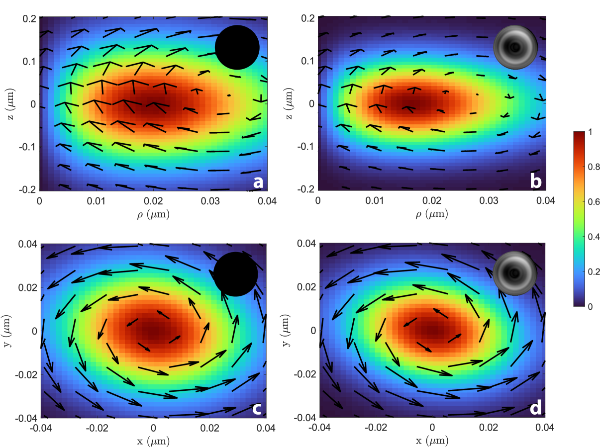
Figure S11: Scattering force-induced vortices in position space. Probability distributions $P_{x}$ (colored map) and currents $\overline{J_{x}}$ (black arrows) in the space $(\rho,z)$ for a 125 nm radius particle trapped at 1 mbar usinf a uniform (a) and an optimized wavefront (b). Probability distributions $P_{x}$ (colored map) and currents $\overline{J_{x}}$ (black arrows) in the space $(x,y)$ for a 125 nm radius particle trapped at 1 mbar using a uniform (c) and an optimized wavefront (d). The amplitudes of the distributions $P_{x}$ are normalized to their maximum values.

Figure S12 compares the vortex amplitudes measured in velocity space for the three phase patterns obtained from the optimizations in Fig. S6, when pressure is reduced. Although the amplitude increases consistently in the space $(v_{x},v_{y})$ compared to the uniform wavefront, this trend is not observed in the space $(v_{\rho},v_{z})$. These results suggest that wavefront shaping can be leveraged to modulate optical scattering effects.

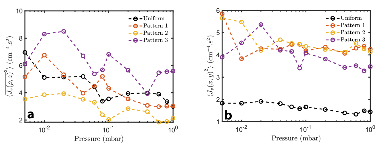
Figure S12: Vortices in velocity space. Amplitude of the vortices as a function of pressure for a 110 nm radius particle, using the wavefronts obtained from the 3 optimizations provided in Fig. S6. Panel a considers the space $(v_{\rho},v_{z})$, while panel b considers the space $(v_{x},v_{y})$.

4 Reducing nonlinearities

The resonance frequency of an optically trapped nanoparticle is expected to remain stable in a harmonic potential. However, as the particle explores larger oscillation amplitudes, nonlinear effects introduce deviations in the resonance frequency. Those nonlinear frequency shifts become particularly significant in the underdamped regime, where low damping leads the system beyond the linear response region.

To characterize the nonlinear effects displayed in Figure 4 of the main text, we analyze the frequency fluctuations as a function of pressure. Following the approach of Ref [11], the resonance frequency is extracted from short-time PSDs computed over 10 ms intervals. The statistical distribution of resonance frequencies was then determined from a 20 s total trace, yielding a dataset of 2000 traces per pressure value. Figure S13a shows histograms of resonance frequencies for a uniform (black) and an optimized (red) wavefront along each axis at 0.1 mbar (using the same nanoparticle studied in the main article). On Figure 4c of the main text, we plot the standard deviation $\sigma_{f}$ of these distributions as a function of pressure. As a consistency check regarding the reduction of nonlinearities, we reproduce in Fig. S13b the same approach using a different 125 nm particle.

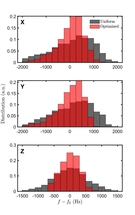
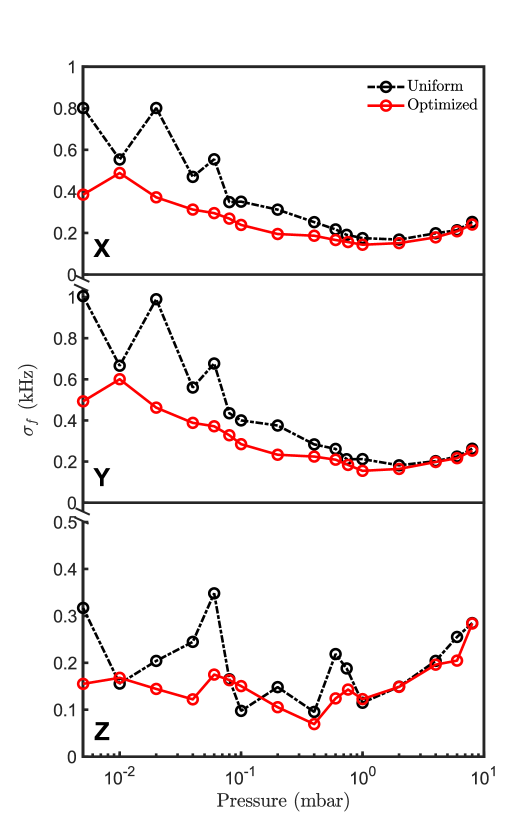
Figure S13: Nonlinearities. a Histograms of the resonance frequency distribution at 0.1 mbar for the three axes, comparing a uniform (black) and an optimized wavefront (red). b Standard deviations, $\sigma_{f}$, of 10 ms time-trace frequency distributions measured along $x$, $y$ and $z$ at different pressures for a uniform (black) and an optimized (red) wavefront.

The purpose of the modulation was to increase the trap stiffness, thereby enhancing the confinement of the particle. Our results show that this increased confinement delays the onset of nonlinearities as the pressure is reduced (Fig. S13b). In the uniform case, nonlinear frequency fluctuations appear at higher pressures, whereas in the optimized configuration, the system remains in the linear regime over a broader pressure range. This demonstrates that wavefront shaping not only enhances trap stiffness but also provides a means to control and mitigate nonlinear effects.

- [1] Cuihong Li, Yuanyuan Ma, Jinchuan Wang, Qianwen Ying, Shaochong Zhu, Zhenhai Fu, Xinbing Jiang, Huan Yang, Tao Liang, Xiaowen Gao, and Huizhu Hu. Morphological tracking and tuning of silica nanoparticles in optomechanical systems for enhanced stable levitation in vacuum. ACS Applied Nano Materials, 7(22):25493–25499, 2024.
- [2] Lukas Novotny and Bert Hecht. Principles of nano-optics. Cambridge university press, 2012.
- [3] Gérard Gouesbet. Generalized lorenz–mie theories and mechanical effects of laser light, on the occasion of arthur ashkin’s receipt of the 2018 nobel prize in physics for his pioneering work in optical levitation and manipulation: A review. Journal of Quantitative Spectroscopy and Radiative Transfer, 225:258–277, 2019.
- [4] Marco Riccardi, Andrei Kiselev, Karim Achouri, and Olivier J.F. Martin. Multipolar expansions for scattering and optical force calculations beyond the long wavelength approximation. Physical Review B, 106, 9 2022.
- [5] Jun Chen, Jack Ng, Zhifang Lin, and C. T. Chan. Optical pulling force. Nature Photonics, 5:531–534, 9 2011.
- [6] Gérard Gouesbet, V.S. De Angelis, and Leonardo André Ambrosio. Optical forces and optical force categorizations on small magnetodielectric particles in the framework of generalized lorenz-mie theory. Journal of Quantitative Spectroscopy and Radiative Transfer, 279:108046, 2022.
- [7] Bo Sun, Jiayi Lin, Ellis Darby, Alexander Y Grosberg, and David G Grier. Brownian vortexes. Physical Review E—Statistical, Nonlinear, and Soft Matter Physics, 80(1):010401, 2009.
- [8] Matthieu Mangeat, Yacine Amarouchene, Yann Louyer, Thomas Guérin, and David S. Dean. Role of nonconservative scattering forces and damping on brownian particles in optical traps. Phys. Rev. E, 99:052107, May 2019.
- [9] Yacine Amarouchene, Matthieu Mangeat, Benjamin Vidal Montes, Lukas Ondic, Thomas Guérin, David S. Dean, and Yann Louyer. Nonequilibrium dynamics induced by scattering forces for optically trapped nanoparticles in strongly inertial regimes. Phys. Rev. Lett., 122:183901, May 2019.
- [10] Erik Hebestreit, Martin Frimmer, René Reimann, Christoph Dellago, Francesco Ricci, and Lukas Novotny. Calibration and energy measurement of optically levitated nanoparticle sensors. Review of Scientific Instruments, 89(3):033111, 03 2018.
- [11] Jan Gieseler, Lukas Novotny, and Romain Quidant. Thermal nonlinearities in a nanomechanical oscillator. Nature Physics, 9:806–810, 2013.