Static black hole horizons in cosmology

Abstract

Despite previous results that rule out the possibility of a static black hole horizon in cosmology we present a black hole metric that has a static horizon whilst mimicking the cosmological behavior at large scales away from the black hole horizon. By a suitable choice of coordinates, we show that it is possible to have a static black hole horizon in cosmology that does not suffer from issues like singularities in curvature invariants at the horizon. The resulting metric is consistent with the Schwarzschild-de Sitter metric for constant Hubble parameter. It should be noted that this metric does not lead to isotropic pressure, i.e. $p_{\perp}\neq p_{r}$ for radial distances comparable to Schwarzschild radius, but for large $r$ the stress tensor (assuming general relativity) tends to the cosmological value. Turning to a more realistic framework, we study the cases of black hole$+$cosmological matter and black hole$+$matter$+$cosmological constant where we assume the pressure component takes its cosmological value and show that although the resulting metric does not have a static horizon, the physical radius of the apparent horizon can tend to a constant value for large cosmological time. This metric does not suffer from issues like a singular horizon for asymptotically vanishing Hubble parameter.

1 Introduction

Black holes are an indispensable part of any textbook on general relativity, which has established the fundamental mathematical tools in our understanding of the universe as a whole or in other words cosmology, and yet a consistent black hole solution (with or without a static horizon) that can be embedded in cosmology is still a matter of debate (see for instance McVittie ; Einstein:1945id ; Kaloper ; Davidson ; Faraoni ; Gaur ; Dahal ; Ion ; Poplawski ; Farrah ). Indeed there are arguments that forbid the existence of black holes with a static horizon, independent of the underlying gravitational theory Davidson Faraoni . Our main initiative in this work is to propose a way out of these no-go results and show that it is possible to find such metrics that behave like a black hole close to the horizon and tend to standard cosmology away from it, meanwhile keeping the horizon static. To this end we use the Painlevé-Gullstrand coordinates for both the black hole and cosmological metrics. In order to achieve a static horizon, we drop one of the assumptions that lead to McVittie's metric. We let $p_{\perp}$ to be different from $p_{r}$ for radial distance $r$ small compared to the cosmological horizon (i.e. in the vicinity of the black hole). Assuming our gravitational theory is general relativity, energy density everywhere is the same as the cosmological value, and the other components also tend to cosmological values for $\frac{l_{1}}{r}\ll 1$, where $l_{1}$ is the static black hole horizon radius. This metric satisfies the null convergence condition, i.e. null energy condition (NEC) outside the horizon, but it violates it inside the black hole horizon. In order to resolve this issue we drop one of our assumptions, namely we allow the energy density to be different from the FLRW one and show that it is in principle possible to have a metric that satisfies NEC inside the black hole horizon as well.

In the second part of this work we consider a more realistic setup with a constant equation of state. Specializing to the case of black hole$+$cosmic matter we find exact black hole solutions and show that it is possible to have a cosmological black hole metric which has an asymptotically (in $t$) constant physical radius. We repeat this calculation for the case of black hole$+$matter$+$cosmological constant and find similar results. In particular we show that the apparent horizons in the latter case tend to the static horizons of Schwarzschild-de Sitter metric for large $t$.

In section II, we provide an intuitive derivation of a black hole metric with a static horizon by cautiously extending the Schwarzschild-de Sitter metric to the case of cosmology with varying Hubble parameter $H$ and show that this metric does not suffer from problems like singularities at the horizon. We show that this metric could be derived via a systematic calculation with some assumptions. We consider the energy conditions for this metric assuming general relativity and find that NEC is violated inside the horizon for this proposal. We then propose a way to respect NEC inside the horizon. In section III, we consider a more realistic framework. We study the case of constant equation of state and the cases of matter and matter$+$cosmological constant separately and find that it is possible to have black hole metrics with apparent horizons that tend to a constant physical radius for large cosmological time. We conclude in section IV.

2 The feasibility of a static horizon

In this section we show that it is in principle possible to have a static black hole horizon in cosmology.

2.1 Extending the Schwarzschild-de Sitter metric

The Schwarzschild metric can be written in Painlevé-Gullstrand coordinates as Painleve Gullstrand

$$ds^{2}=-(1-\frac{l_{s}}{r})dt^{2}+2\sqrt{\frac{l_{s}}{r}}drdt+dr^{2}+r^{2}d\Omega_{2}^{2}.$$ (1)

On the other hand, the cosmological FLRW metric can be written in Painlevé-Gullstrand coordinates as Gaur2

$$ds^{2}=-(1-\frac{\dot{a}^{2}}{a^{2}}r^{2})dt^{2}-2\frac{\dot{a}}{a}rdtdr+dr^{2}+r^{2}d\Omega_{2}^{2}.$$ (2)

where $a(t)$ is the scale factor.

This coordinate system is specially suitable for writing a metric that interpolates between the cosmological metric and the Schwarzschild metric due to the time-independent radial factor of angular coordinates.

Abiding by the requirement that any cosmological black hole metric should tend to the Schwarzschild-de Sitter solution, in the limit of constant Hubble parameter, we first consider the Schwarzschild-de Sitter metric in Painlevé-Gullstrand coordinates Gaur2

$$ds^{2}=-(1-\frac{l_{s}}{r}-\frac{r^{2}}{l^{2}})dt^{2}-2\sqrt{\frac{l_{s}}{r}+\frac{r^{2}}{l^{2}}}dtdr+dr^{2}+r^{2}d\Omega_{2}^{2},$$ (3)

and factorize the $g_{tt}$ part to its roots as

$$1-\frac{l_{s}}{r}-\frac{r^{2}}{l^{2}}=\frac{l_{s}}{l_{1}}(1-\frac{l_{1}}{r})(1-\frac{r}{l_{2}})(1+\frac{r}{l_{1}+l_{2}}).$$ (4)

Here $l_{1}$ and $l_{2}$ are respectively the black hole and cosmological horizons which obey

$$l_{s}=\frac{l_{1}l_{2}(l_{1}+l_{2})}{(l_{1}+l_{2})^{2}-l_{1}l_{2}},\qquad l^{2}=(l_{1}+l_{2})^{2}-l_{1}l_{2}.$$ (5)

Then the the metric is brought to the form

$$ds^{2}=-\frac{l_{s}}{l_{1}}\Big{(}1-\frac{l_{1}}{r}-\frac{r^{2}-l_{1}^{2}}{l_{2}(l_{1}+l_{2})}\Big{)}dt^{2}-2\sqrt{\frac{l_{s}}{l_{1}}\frac{l_{1}}{r}+\frac{r^{2}}{l^{2}}}dtdr+dr^{2}+r^{2}d\Omega_{2}^{2}.$$ (6)

Relating $l_{2}$ and $l_{s}$ to $l_{1}$ and $l$ we can write this as

$$ds^{2}=-\big{(}1-(\frac{l_{1}}{l})^{2}\big{)}\Big{(}1-\frac{l_{1}}{r}-\frac{r^{2}-l_{1}^{2}}{l^{2}-l_{1}^{2}}\Big{)}dt^{2}-2\sqrt{\big{(}1-(\frac{l_{1}}{l})^{2}\big{)}\frac{l_{1}}{r}+\frac{r^{2}}{l^{2}}}dtdr+dr^{2}+r^{2}d\Omega_{2}^{2}.$$ (7)

which is useful for our purposes since the dependence on the two horizons is explicit and they are written in a disentangled fashion.

Using this analogy we propose a metric for a spherically symmetric black hole with a static horizon in cosmology as

$$ds^{2}=-(1-\frac{l_{1}^{2}\dot{a}^{2}}{a^{2}})\Big{(}1-\frac{l_{1}}{r}-\frac{r^{2}-l_{1}^{2}}{\frac{a^{2}}{\dot{a}^{2}}-l_{1}^{2}}\Big{)}dt^{2}\\ -2\sqrt{\big{(}1-\frac{l_{1}^{2}\dot{a}^{2}}{a^{2}}\big{)}\frac{l_{1}}{r}+\frac{r^{2}\dot{a}^{2}}{a^{2}}}dtdr+dr^{2}+r^{2}d\Omega_{2}^{2}.$$ (8)

The metric (8) can be written in a more suggestive form as

$$ds^{2}=-(1-h^{2})dt^{2}-2hdtdr+dr^{2}+r^{2}d\Omega_{2}^{2}.$$ (9)

where

$$h=\sqrt{\frac{l_{1}}{r}+\frac{r^{3}-l_{1}^{3}}{r}\frac{\dot{a}^{2}}{a^{2}}}.$$ (10)

This metric has the property that the black hole and cosmological horizons are detached and it has an static horizon at $r=l_{1}$. Also if we replace $\frac{a}{\dot{a}}$ with de Sitter length $l$ for the cosmological constant, we recover the Schwarzschild-de Sitter metric.

In the large $r$ limit the metric tends to the cosmological metric (2) with $t$ the FLRW time. In the small $r$ limit the metric tends to the Schwarzschild metric (1) with Painlevé-Gullstrand time. We note that using this metric, the FLRW time is compared with Painlevé-Gullstrand time in Schwarzschild metric and not the static Schwarzschild time.

Since the horizon is a little obscure in these coordinates, we can change variables to remove the $g_{tr}$ part of the metric. Writing $t=\gamma(\tau,r)$ the $g_{tr}$ component of the metric becomes

$$g_{tr}=-2\dot{\gamma}((1-h^{2})\gamma^{\prime}+h).$$ (11)

Therefore to remove this we choose $\gamma$ such that

$$\gamma^{\prime}=-\frac{h}{1-h^{2}}.$$ (12)

Then the metric becomes

$$ds^{2}=-(1-h^{2})\dot{\gamma}^{2}d\tau^{2}+\frac{dr^{2}}{1-h^{2}}+r^{2}d\Omega_{2}^{2}.$$ (13)

This metric has a static horizon at $r=l_{1}$ where $h=1$ independent of $\tau$.

We can see that the Ricci scalar and curvature invariants like $R^{\mu\nu}R_{\mu\nu}$ and $R^{\mu\nu\rho\sigma}R_{\mu\nu\rho\sigma}$ remain finite at the black hole horizon. In particular we have at the horizon $r=l_{1}$

$$R|_{r=l_{1}}=-6\,l_{1}\frac{\dot{a}^{3}}{a^{3}}+6\,l_{1}\frac{\dot{a}\ddot{a}}{a^{2}}+12\frac{\dot{a}^{2}}{a^{2}}.$$ (14)

For visualization we sketch the Ricci scalar, $R^{\mu\nu}R_{\mu\nu}$, $R^{\mu\nu\rho\sigma}R_{\mu\nu\rho\sigma}$ as a function of $r$ for fixed $l_{1}=1$ and $t=10$ for both radiation and matter dominated cases in Figure 1.

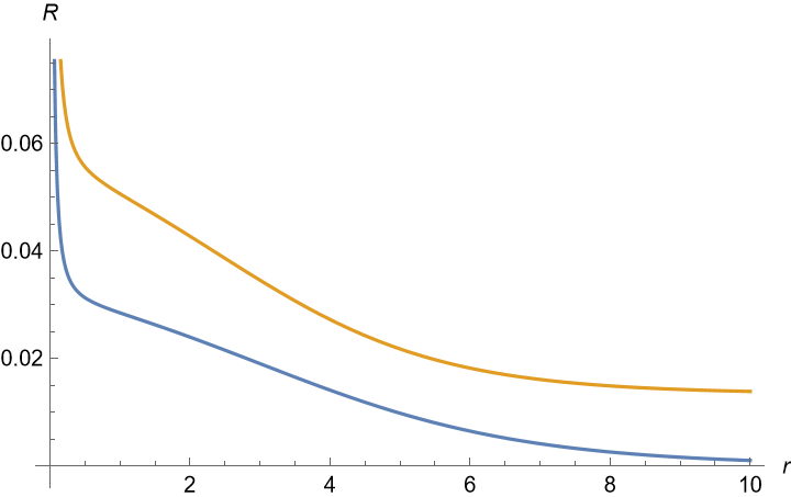
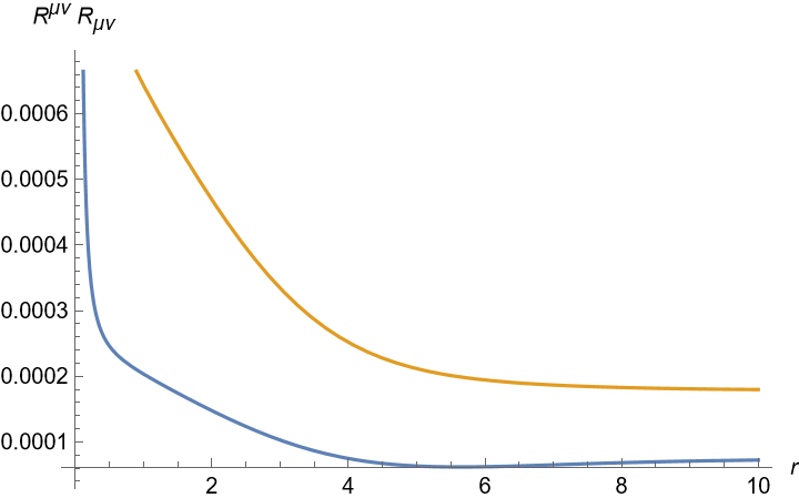
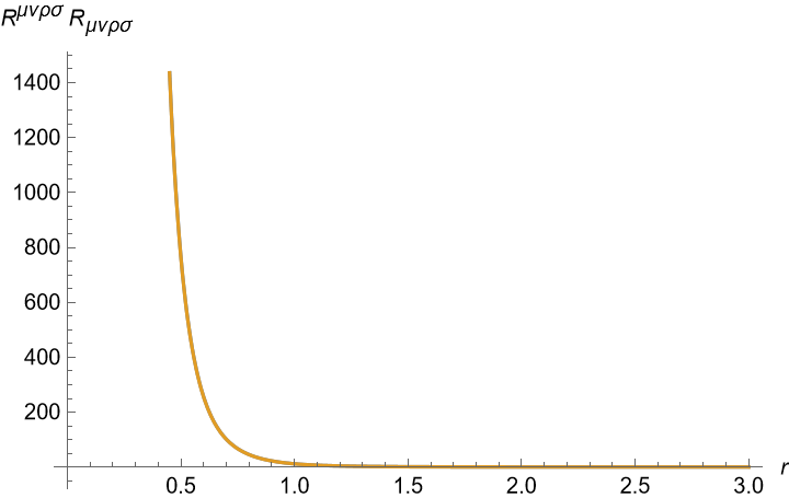
Figure 1: The Ricci scalar, $R^{\mu\nu}R_{\mu\nu}$, $R^{\mu\nu\rho\sigma}R_{\mu\nu\rho\sigma}$ as a function of $r$, for $l_{1}=1$ and $t=10$, with blue and orange curves related to radiation and matter respectively. In the last plot, radiation and matter curves are almost coincident. These plots represent the observation that this metric has a singularity only at $r=0$ and not at the black hole horizon.

Another interesting property is that $T^{t}_{r}$ which we find from requiring Einstein's equation is zero. In other words there is no flux of energy in radial direction. This is the requirement also present in McVittie's solution. On the other hand, the large $r$ limit of stress tensor tends to the cosmological values.

Explicitly we have

$$G^{t}_{t}=-3\frac{\dot{a}^{2}}{a^{2}},\quad\quad G^{t}_{r}=0,$$ (15)

$$G^{r}_{t}=-2\,r\big{(}1-\frac{l_{1}^{3}}{r^{3}}\big{)}\Big{(}\frac{\dot{a}^{3}}{a^{3}}-\frac{\dot{a}\ddot{a}}{a^{2}}\Big{)}=g^{tr}(G^{r}_{r}-G^{t}_{t}),$$ (16)

and

$$G^{\theta}_{\theta}=G^{\phi}_{\phi}=-3\frac{\dot{a}^{2}}{a^{2}}-\frac{l_{1}(l_{1}^{3}-7r^{3})}{2r^{3}g_{tr}^{3}}\Big{(}\frac{\ddot{a}\dot{a}}{a^{2}}-\frac{\dot{a}^{3}}{a^{3}}\Big{)}-\frac{(l_{1}^{3}-r^{3})(l_{1}^{3}-4r^{3})}{2r^{3}g_{tr}^{3}}\Big{(}\frac{\dot{a}^{5}}{a^{5}}-\frac{\ddot{a}\dot{a}^{3}}{a^{4}}\Big{)}$$ (17)

We can see that (assuming the gravitational theory is general relativity,) the radial pressure for small $r$ is not equal to angular pressure, i.e. we do not have $p_{\perp}=p_{r}$. This shows that the metric close to the black hole is not isotropic at every point. But since the $G^{\mu}_{\nu}$ tends to the cosmological value for large $\frac{r}{l_{1}}$ this property ($p_{\perp}=p_{r}$) is restored in this limit.

2.2 A systematic derivation

Having found the metric (8), we show that it could have been derived in a more systematic way uniquely. We begin with the Painlevé-Gullstrand-like metric ansatz

$$ds^{2}=-f(t,r)dt^{2}-2h(t,r)dtdr+dr^{2}+r^{2}d\Omega_{2}^{2},$$ (18)

and consider the following assumptions:

$a)$ There is no flux of energy in radial direction, i.e. we assume $T^{t}_{r}=0$.

$b)$ There is a static horizon at $r=l_{1}$, such that $g_{tt}|_{r=l_{1}}=0$.

$c)$ We assume the energy density is the same as the FLRW one, i.e. we assume $G^{t}_{t}=-3\frac{\dot{a}^{2}}{a^{2}}$.

$d)$ The metric at large $r$ tends to the cosmological FLRW metric.

We note that compared to McVittie's assumptions, we have dropped the $p_{\perp}=p_{r}$ assumption and instead we have added assumption b.

Using the metric (18), we have

$$G^{t}_{r}=-\frac{h(f^{\prime}+2hh^{\prime})}{r(f+h^{2})^{2}},$$ (19)

where ^′ denotes derivative with respect to $r$. Requiring this to vanish considering the first assumption, we find

$$f(t,r)=\gamma(t)-\omega(t,r),$$ (20)

where we have defined $\omega(t,r)=h^{2}(t,r)$. We then consider the second assumption. From this and using (20) we require

$$\omega(t,l_{1})=\gamma(t).$$ (21)

Considering assumption c, we have

$$G^{t}_{t}=-\frac{\omega(t,r)+r\omega^{\prime}(t,r)}{r^{2}\omega(t,l_{1})}=-3\frac{\dot{a}^{2}}{a^{2}}.$$ (22)

Integrating we find

$$\omega(t,r)=\omega(t,l_{1})r^{2}\frac{\dot{a}^{2}}{a^{2}}+\frac{c(t)}{r}.$$ (23)

Considering assumption d we have $\omega(t,l_{1})=1$ and from this considering (23) at $r=l_{1}$, we have

$$c(t)=l_{1}\big{(}1-\frac{\dot{a}^{2}}{a^{2}}l_{1}^{2}\big{)}.$$ (24)

Therefore with these assumptions the proposed metric (8) is unique.

2.3 Energy conditions

In this section we study the energy conditions for the stress tensor corresponding to this metric assuming the gravitational theory is general relativity.

We begin with the weak energy condition that states for every timeline vector $k^{\mu}$ we should have

$$T_{\mu\nu}k^{\mu}k^{\nu}\geq 0$$ (25)

Considering the case where only $k^{t}=1$ and $k^{r}$ are nonzero we have for the vector $k^{\mu}$ the inequality

$$g_{tt}+2g_{tr}k^{r}+g_{rr}(k^{r})^{2}<0$$ (26)

which using $g_{tt}=-1+g_{tr}^{2}$ leads to

$$-1-g_{tr}<k^{r}<1-g_{tr}.$$ (27)

Using these marginal values of $k^{r}$, we find that in both cases

$$T_{\mu\nu}k^{\mu}k^{\nu}=\frac{2(l_{1}^{3}-r^{3})(\dot{a}^{2}-a\ddot{a})}{r^{2}a^{3}g_{tr}}.$$ (28)

For a typical power-law scale factor, this is always positive outside the horizon and negative inside the horizon (since $g_{tr}<0$). Therefore assuming the gravitational theory is general relativity, the stress tensor corresponding to this metric does not satisfy the weak and null energy conditions inside the black hole horizon.

Considering the strong energy condition we find that it is violated in the vicinity of the black hole (see figure 2).

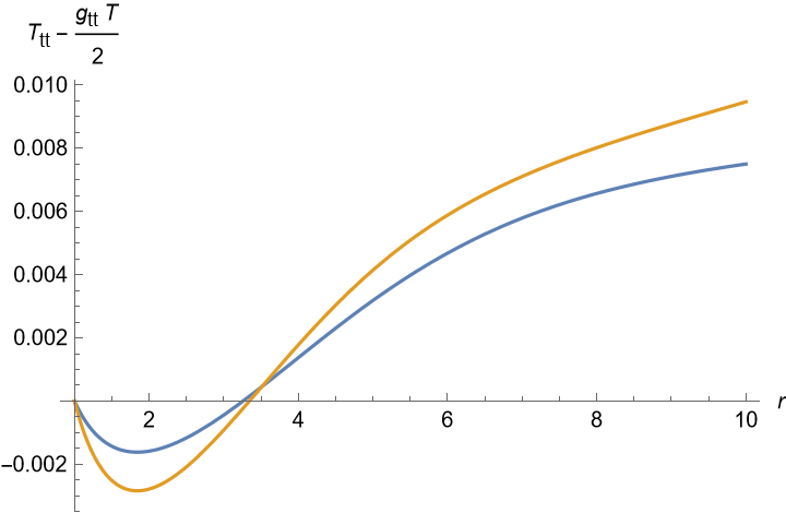
Figure 2: Here we have plotted $T_{tt}-\frac{1}{2}g_{tt}T$ as a function of $r$. We have chosen $l_{1}=1$ and $t=10$. The blue and orange curves respectively correspond to radiation and matter dominated scale factors. The strong energy condition is violated in the black hole's vicinity.

2.4 NEC and static horizon

Here we drop assumption c mentioned in the previous section to see if we can find a metric with a static horizon that respects NEC. We begin with the metric

$$ds^{2}=-f(t,r)dt^{2}-2h(t,r)dtdr+dr^{2}+r^{2}d\Omega_{2}^{2}.$$ (29)

We still have (20), which considering assumption d takes the form

$$f(t,r)=1-h^{2}(t,r).$$ (30)

We then consider NEC. It can be shown that NEC requires $\dot{h}(t,r)<0$ everywhere, (as we have $T_{\mu\nu}k^{\mu}k^{\nu}=-2\frac{\dot{h}}{r}$). Since we assume to have a static horizon at some $r=l_{1}$ (for which $h(t,l_{1})=1$), at the horizon $\dot{h}$ becomes zero and the only way it does not become positive below the horizon is to have $\dot{h}^{\prime}(t,l_{1})=0$ at the horizon.

One possible metric which respects NEC and assumptions a,b,d has

$$h(t,r)=\sqrt{\frac{l_{1}}{r}+r^{2}(1-\frac{l_{1}^{3}}{r^{3}})\frac{\dot{a}^{2}}{a^{2}}+l_{1}^{2}(1-\frac{l_{1}^{3}}{r^{3}})(\frac{1}{l_{0}^{2}}-\frac{\dot{a}^{2}}{a^{2}})}.$$ (31)

Here $l_{0}$ is related to the cosmological constant $\Lambda=\frac{3}{l_{0}^{2}}$.

We have

$$\dot{h}=-\frac{(l_{1}-r)^{2}(l_{1}+r)(l_{1}^{2}+l_{1}r+r^{2})}{r^{3}h}\big{(}\frac{\dot{a}^{3}}{a^{3}}-\frac{\dot{a}\ddot{a}}{a^{2}}\big{)},$$ (32)

which is negative for all $r$.

3 The case of constant equation of state

In this section we consider the possibility that the black hole metric respects the cosmological stress tensor equation of state. Assuming $T^{t}_{r}=0$, from (19) we find

$$f(t,r)=\gamma(t)-h^{2}(t,r).$$ (33)

We do not consider any further assumptions and continue our analysis for the case of constant equation of state.

We assume $p_{\perp}=p_{r}=\omega\rho$. Assuming $G^{r}_{t}=g^{tr}(G^{r}_{r}-G^{t}_{t})$ , we have from Einstein equations

$$G^{r}_{t}=\frac{h}{r\gamma^{2}}(2\gamma\dot{h}-h\dot{\gamma})=-\frac{h}{\gamma^{2}}\kappa_{4}(1+\omega)\rho,$$ (34)

and therefore

$$\frac{1}{r}(2\gamma\dot{h}-h\dot{\gamma})=-\kappa_{4}(1+\omega)\rho.$$ (35)

On the other hand from $G^{t}_{t}=-\kappa_{4}\rho$ and (35) we find

$$h^{2}+2rhh^{\prime}+\frac{2r\gamma^{2}\dot{h}-rh\gamma\dot{\gamma}}{1+\omega}=0.$$ (36)

We also have by considering $G^{r}_{r}=\kappa_{4}\omega\rho$,

$$h^{2}+2rhh^{\prime}+\frac{2r\dot{h}-rh\frac{\dot{\gamma}}{\gamma}}{1+\omega}=0.$$ (37)

Using (36) and (37) we find

$$(2r\dot{h}-rh\frac{\dot{\gamma}}{\gamma})(\gamma^{2}-1)=0.$$ (38)

So we either have $\gamma^{2}=1$ or $2\frac{\dot{h}}{h}=\frac{\dot{\gamma}}{\gamma}$.

The second possibility requires $h^{2}=c(r)\gamma(t)$. Using (36) again we find $c(r)=\frac{l_{s}}{r}$ where $l_{s}$ is a constant length and the metric takes the form

$$ds^{2}=-\gamma(t)(1-\frac{l_{s}}{r})dt^{2}-2\sqrt{\frac{l_{s}}{r}\gamma(t)}dtdr+dr^{2}+r^{2}d\Omega^{2},$$ (39)

which is the Schwarzschild metric in Painlevé-Gullstrand coordinates (This is evident by changing $t$ to $t^{\prime}$ such that $dt^{\prime}=\sqrt{\gamma(t)}dt$). Therefore, in order to find a cosmological black hole metric, our preference will be $\gamma(t)=1$ in what follows.

Assuming $\gamma(t)=1$, we have from the $G^{0}_{0}$ component of Einstein equations and (35)

$$h^{2}+2rhh^{\prime}+\frac{2}{1+\omega}r\dot{h}=0.$$ (40)

Considering the $G^{\theta}_{\theta}$ component we find

$$\partial_{r}(r\dot{h}+rhh^{\prime}+\frac{h^{2}}{2})=-\kappa_{4}r\omega\rho=\frac{1}{r}(h^{2}+2rhh^{\prime}+2r\dot{h}),$$ (41)

where we used the $G^{r}_{r}$ component as well. In the following, we consider the case of $\omega=0$ and $\omega\neq 0$ separately.

3.1 The case of $\omega\neq 0$

In this case, from (41) we find

$$h^{2}+2rhh^{\prime}+2r\dot{h}=\frac{2\omega}{1+\omega}\dot{\zeta}(t)r^{2}.$$ (42)

Here $\zeta(t)$ is some function of $t$ and we have chosen the coefficient and a derivative with respect to $t$ for later convenience.

Subtracting (40) from (42) we further find

$$h=\zeta(t)r+\alpha(r).$$ (43)

Using (40) again we find

$$3\zeta^{2}(t)r^{2}+4r\zeta(t)\alpha(r)+2r^{2}\zeta(t)\alpha^{\prime}(r)+\frac{2}{1+\omega}r^{2}\dot{\zeta}+\alpha^{2}(r)\\ +2r\alpha(r)\alpha^{\prime}(r)=0.$$ (44)

The only nontrivial solution of this equation which is of cosmological interest is $\alpha(r)=0$, $\zeta(t)=\frac{2}{3(1+\omega)t}$. Therefore we do not have a cosmological black hole solution that satisfies $p_{r}=p_{\perp}=\omega\rho$ for $\omega\neq 0$.

3.2 The case of matter with $\omega=0$

To simplify our analysis, we change the coordinates to a semi-homogeneous form by setting $r=a(t,R)R$, demanding the transformed metric to be diagonal by setting $h=R\dot{a}$. Therefore, the metric becomes simply

$$ds^{2}=-dt^{2}+(a+Ra^{\prime})^{2}dR^{2}+a^{2}R^{2}d\Omega_{2}^{2},$$ (45)

where $a^{\prime}=\partial_{R}a$. We note that if $a$ was independent of $R$, this was the FLRW metric. In this coordinate $T^{R}_{t}=T^{t}_{R}=0$ and the Einstein equations become

$$\frac{3a\dot{a}^{2}+R\,a^{\prime}\dot{a}^{2}+2R\,a\dot{a}\dot{a}^{\prime}}{a^{2}(a+R\,a^{\prime})}=\frac{\partial_{R}(R^{3}a\dot{a}^{2})}{R^{2}a^{2}(a+R\,a^{\prime})}=\kappa_{4}\rho,$$ (46)

$$(\frac{\dot{a}}{a})^{2}+2\frac{\ddot{a}}{a}=-\kappa_{4}p_{r},$$ (47)

$$\frac{\dot{a}^{2}+R\,\dot{a}\dot{a}^{\prime}+2a\ddot{a}+R\,a^{\prime}\ddot{a}+R\,a\ddot{a}^{\prime}}{a(a+R\,a^{\prime})}=-\kappa_{4}p_{\perp}.$$ (48)

In this section we consider the case of a Schwarzschild black hole immersed in cosmological matter. In this case we have $p_{r}=p_{\perp}=0$. From stress energy conservation we can find the structure of $\rho$. We have

$$\frac{\dot{\rho}}{\rho}+2\frac{\dot{a}}{a}+\frac{\dot{a}+R\,\dot{a}^{\prime}}{a+R\,a^{\prime}}=0,$$ (49)

and we find

$$\kappa_{4}\rho=\frac{\beta(R)}{a^{2}(a+R\,a^{\prime})}.$$ (50)

From (46) we can write

$$R^{3}a\dot{a}^{2}=\int^{R}dR^{\prime}\,R^{\prime 2}\beta(R^{\prime}).$$ (51)

From (47) we find

$$a(t,R)=c(R)\,\big{(}\frac{3}{2}t-b(R)\big{)}^{2/3},$$ (52)

and this also satisfies (48). Using (51) this means

$$R^{3}c(R)^{3}=\int^{R}dR^{\prime}\,R^{\prime 2}\beta(R^{\prime}).$$ (53)

We first re-derive the Schwarzschild metric in these coordinates. If we only had a point mass contribution to $\rho$, this equation would lead to

$$c(R)=\frac{l_{s}^{1/3}}{R}$$ (54)

or

$$a(t,R)=\frac{l_{s}^{1/3}}{R}(\frac{3}{2}t-b(R))^{2/3}.$$ (55)

In our original central coordinate this means that we had

$$h=R\,\dot{a}=\frac{l_{s}^{1/3}}{(\frac{3}{2}t-b(R))^{1/3}}=\sqrt{\frac{l_{s}}{r}}$$ (56)

where in the last equality we used $r=R\,a$. We see that this simple case corresponds to the Schwarzschild metric in Painlevé-Gullstrand coordinates. We also note that in this coordinate the black hole singularity is at the surface $\frac{3}{2}t-b(R)=0$. There is a freedom in our choice of $b(R)$.

Now returning to the case of black hole in matter-dominated cosmology we can add a term related to the cosmological matter density to $\beta(R)$. We note that in the asymptotic case we should have $\kappa_{4}\beta(R)=\beta_{0}$ where $\beta_{0}$ is a constant. Considering that this is also the case for large $t$ we set $\kappa_{4}\beta(R)=\beta_{0}$ and find

$$c(R)=\left(\frac{l_{s}}{R^{3}}+\frac{\beta_{0}}{3}\right)^{1/3},$$ (57)

and

$$h=R\dot{a}=\frac{\left(l_{s}+\frac{\beta_{0}}{3}R^{3}\right)^{1/3}}{\left(\frac{3}{2}t-b(R)\right)^{1/3}}=\frac{r}{\frac{3}{2}t-b(R)}.$$ (58)

The apparent horizon is at $h=1$. Therefore we have

$$r_{H}=\frac{3}{2}t-b(R_{H}).$$ (59)

On the other hand, using $r=Ra$ we have

$$r_{H}=(l_{s}+\frac{\beta_{0}}{3}R^{3})^{1/3}(\frac{3}{2}t-b(R))^{2/3},$$ (60)

and using (59) we can write

$$r_{H}=l_{s}+\frac{\beta_{0}}{3}R_{H}^{3}.$$ (61)

As an example, if we choose $b(R)=\frac{\kappa l_{s}^{4}}{R^{3}}-d$, using (59) and (61) we can find

$$r_{H}=l_{s}+\frac{\frac{\beta_{0}}{3}\kappa l_{s}^{4}}{\frac{3}{2}t+d-r_{H}},$$ (62)

with solutions

$$r_{H}(t)=\frac{1}{4}\big{(}3t+2d+2l_{s}\pm\sqrt{(3t+2d-2l_{s})^{2}-\frac{16}{3}\beta_{0}\kappa l_{s}^{4}}\big{)}.$$ (63)

For large $t$ one of these tends to $r_{H}=\frac{3t}{2}$, which is the cosmological horizon, and the other tends to $r_{H}=l_{s}$, which is the black hole horizon. Therefore, for large $t$ we effectively have a static black hole horizon.

We had freedom in our choice of $b(R)$. Requiring that the metric tends to the cosmological metric for large $R$ will force us to choose $b(R)$ such that it tends to a constant for large $R$. The surface $\frac{3t}{2}=b(R)$, $r=0$ is where both the cosmological singularity and black hole singularity reside. We see that the choice for $b(R)$ fixes both the singularity and the evolution of the black hole in $t$.

We can prove that generically the resulting apparent horizon in this case will be dynamical (apart from the asymptotic behavior). To see this we write

$$h=R\dot{a}=\frac{Rc(R)}{(\frac{3t}{2}-b(R))^{1/3}}=\frac{r}{\frac{3t}{2}-b(R)}.$$ (64)

Requiring $h=1$ at the horizon and considering $r=Ra$, we can write

$$r_{H}=(R_{H}c(R_{H}))^{3}=\int^{R_{H}}dR^{\prime}R^{\prime 2}\beta(R^{\prime}),$$ (65)

$$r_{H}=\frac{3t}{2}-b(R_{H}).$$ (66)

Taking a time derivative, we find

$$\dot{r}_{H}=\dot{R}_{H}R_{H}^{2}\beta(R_{H})=\frac{3}{2}-\dot{R}_{H}b^{\prime}(R_{H}).$$ (67)

From this, we can see that it is impossible to have $\dot{r}_{H}=0$ exactly.

3.3 The case of matter$+$cosmological constant

In this case from $-\kappa_{4}p_{r}=\frac{3}{l^{2}}$ and (47) we find

$$a(t,R)=c(R)\sinh^{2/3}\left(\frac{3t}{2l}-\frac{b(R)}{l}\right).$$ (68)

We again have (49) and (50) for the matter part of energy density. From (46) we can write

$$\partial_{R}(R^{3}a\dot{a}^{2})=R^{2}\beta(R)+\frac{3}{l^{2}}R^{2}a^{2}(a+Ra^{\prime}).$$ (69)

Using (68) we find

$$\frac{3}{l^{2}}c^{2}(R)(c(R)+Rc^{\prime}(R))=\beta(R)\,,$$ (70)

or alternatively

$$\frac{1}{l^{2}}\partial_{R}(R^{3}c^{3})=R^{2}\beta(R).$$ (71)

We are again left with two unfixed functions of $R$, namely $b(R)$ and $\beta(R)$. One can use the degree of freedom in choosing the $R$ coordinate to fix one of them.

If we assume $\beta(R)=\beta_{0}$ to be a constant we find

$$c(R)=\left(\frac{l_{s}l^{2}}{R^{3}}+\frac{\beta_{0}\,l^{2}}{3}\right)^{1/3}$$ (72)

By studying $h=R\,\dot{a}$ one can see that for $\beta_{0}=0$, which is the case of pure cosmological constant, $l_{s}$ is the Schwarzschild radius, i.e. for $\beta_{0}=0$ we have

$$h|_{\beta_{0}=0}=R\,\dot{a}=\sqrt{\frac{l_{s}}{r}+\frac{r^{2}}{l^{2}}}.$$ (73)

We study the apparent horizon, which is located at $h=1$. We have

$$h=R\,\dot{a}=\frac{r}{l}\coth\left(\frac{3t}{2l}-\frac{b(R)}{l}\right).$$ (74)

From this at $h=1$ we find

$$\sinh^{2}\left(\frac{3t}{2l}-\frac{b(R)}{l}\right)=\frac{\frac{r_{H}^{2}}{l^{2}}}{1-\frac{r_{H}^{2}}{l^{2}}}.$$ (75)

Using (68) and (72) and assuming $b(R)$ behaves such that the location of the horizon for large $t$ goes to small $R_{H}$, we can write for large $t$

$$r_{H}\approx(l_{s}l^{2})^{1/3}\Big{(}\frac{\frac{r_{H}^{2}}{l^{2}}}{1-\frac{r_{H}^{2}}{l^{2}}}\Big{)}^{1/3},$$ (76)

and

$$\frac{l_{s}}{r_{H}}+\frac{r_{H}^{2}}{l^{2}}=1.$$ (77)

The smallest root of this equation is the black hole horizon. This means that the location of the black hole horizon for large $t$ tends to its Schwarzschild-de Sitter counterpart.

If we require that the observer is at large $R$ then we should choose $b(R)$ such that the cosmological behavior is dominant for large $R$. The location of singularity is at $\frac{3t}{2}=b(R)$. Choosing as an example $b(R)=\frac{\kappa l_{s}^{4}}{R^{3}}-d$, the location of singularity tends to $R=0$ for large $t$ and to a constant $R$ for small $t$.

4 Summary

Despite the recent claim that black hole horizons should be cosmologically coupled, in this work, we provide counterexamples for cosmological black hole metrics that have static or asymptotically static horizons.

In the first part of this work, we propose a black hole metric with a static horizon embedded in FLRW cosmology. This metric has the following properties:

$a)$ It has a static horizon with no curvature singularity.

$b)$ It tends to the cosmological FLRW metric for large physical radius $r$.

$c)$ The energy density is the same as the cosmological case, but the pressure is different.

$d)$ The stress tensor also tends to the FLRW values for large $r$.

$e)$ If we fix the sign of $g_{tr}$ to be negative, the resulting metric satisfies the null convergence condition outside the horizon but violates it inside the horizon.

The corresponding stress tensor, assuming general relativity, violates the strong energy condition in the vicinity of the black hole.

$f)$ For the case of a constant Hubble parameter, it is equal to the Schwarzschild-de Sitter metric.

Since our proposed metric violates NEC inside the horizon, we drop one of our assumptions and see that it is in principle possible to find a cosmological metric with a static horizon that satisfies NEC everywhere.

In the second part of this work we considered a more realistic framework with a constant equation of state (for the cases of matter and radiation) and show that we have no black hole solutions for the case of $\omega\neq 0$. For the case of matter with $\omega=0$, we derived the black hole metric consistent with this assumption. The crucial feature of this metric is that despite having an asymptotically vanishing Hubble parameter, we have no singularities at the horizon.

We also studied the case of matter$+$cosmological constant where we assumed the pressure component remains equal to the constant cosmological value. In all of these cases we show that the black hole horizon can asymptotically (for large $t$) tend to a static horizon.

References

- (1) G. C. McVittie, ``The mass-particle in an expanding universe", Mon. Not. R. Astron. Soc. 93, 325 (1933); Ap. J. 143, 682 (1966); General Relativity and Cosmology, 2nd Edition, University of Illinois Press 1962.
- (2) A. Einstein and E. G. Straus, ``The influence of the expansion of space on the gravitation fields surrounding the individual stars,'' Rev. Mod. Phys. 17, 120-124 (1945)
- (3) Nemanja Kaloper, Matthew Kleban, Damien Martin, ``McVittie's Legacy: Black Holes in an Expanding Universe", Phys.Rev.D 81 (2010) 104044.
- (4) Aharon Davidson, Shimon Rubin, Yosef Verbin, ``Can an evolving Universe host a static event horizon?", Phys. Rev. D 86, 104061 (2012).
- (5) Valerio Faraoni, Massimiliano Rinaldi, ``Black hole event horizons are cosmologically coupled", arXiv:2407.14549v2.
- (6) Rudeep Gaur, Matt Visser, ``Black holes embedded in FLRW cosmologies", Phys. Rev. D 110, 043529.
- (7) Pravin K. Dahal, Swayamsiddha Maharana, Fil Simovic, Ioannis Soranidis, Daniel R. Terno, ``Models of cosmological black holes", Phys. Rev. D 110, 044032.
- (8) Ion I. Cotăescu, ``New one-parameter models of dynamical particles in spatially flat FLRW space-times", Eur. Phys. J. C 84, 819 (2024).
- (9) Nikodem Popławski, ``Black holes in the expanding Universe", Class. Quantum Grav. 42, 065017 (2025).
- (10) Duncan Farrah et al, ``Observational Evidence for Cosmological Coupling of Black Holes and its Implications for an Astrophysical Source of Dark Energy", 2023 ApJL 944 L31.
- (11) Paul Painlevé, "La mécanique classique et la théorie de la relativité", C. R. Acad. Sci. (Paris) 173, 677–680(1921).
- (12) Allvar Gullstrand. "Allgemeine Lösung des statischen Einkörperproblems in der Einsteinschen Gravitationstheorie". Arkiv för Matematik, Astronomi och Fysik. 16 (8): 1–15.
- (13) Rudeep Gaur, Matt Visser, ``Cosmology in Painlevé-Gullstrand coordinates", JCAP09(2022)030.