BrightCookies at SemEval-2025 Task 9: Exploring Data Augmentation for Food Hazard Classification

Abstract

This paper presents our system developed for the SemEval-2025 Task 9: The Food Hazard Detection Challenge. The shared task’s objective is to evaluate explainable classification systems for classifying hazards and products in two levels of granularity from food recall incident reports. In this work, we propose text augmentation techniques as a way to improve poor performance on minority classes and compare their effect for each category on various transformer and machine learning models. We explore three word-level data augmentation techniques, namely synonym replacement, random word swapping, and contextual word insertion. The results show that transformer models tend to have a better overall performance. None of the three augmentation techniques consistently improved overall performance for classifying hazards and products. We observed a statistically significant improvement (P < 0.05) in the fine-grained categories when using the BERT model to compare the baseline with each augmented model. Compared to the baseline, the contextual words insertion augmentation improved the accuracy of predictions for the minority hazard classes by 6%. This suggests that targeted augmentation of minority classes can improve the performance of transformer models.

BrightCookies at SemEval-2025 Task 9: Exploring Data Augmentation for Food Hazard Classification

Foteini Papadopoulou^1,2, Osman Mutlu¹, Neris Özen¹, Bas H.M. van der Velden¹, Iris Hendrickx², Ali Hürriyetoğlu^{1 1}Wageningen Food Safety Research, The Netherlands ²Centre for Language Studies, Radboud University, The Netherlands Correspondence: ali.hurriyetoglu@wur.nl

1 Introduction

Foodborne diseases affect millions of people every year. The World Health Organization highlights that food contamination leads to more than 200 diseases, resulting in severe health complications and affecting the socioeconomic stability of communities and nations World Health Organization (2024). There is a vast amount of publicly available information on food safety-related websites. Given the importance of early detection of food hazards, there is a need to timely and accurately analyze all this publicly available information to detect food hazards.

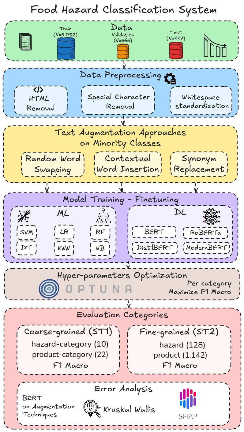
Figure 1: An overview of our developed system’s architecture.

The SemEval-2025 Task 9: Food Hazard Detection Challenge Randl et al. (2025) was proposed to facilitate automated classification of food hazards in food safety-related documents. It stimulates research that combines food safety and natural language processing (NLP) for explainable multi-class classification of food recall incident reports. SemEval-2025 Task 9 includes two sub-tasks: classifying coarse food hazard and product categories (ST1) (hazard-category, product-category), and fine-grained hazard and product categories (ST2) (hazard, product).

A significant challenge with the SemEval-2025 Task 9 dataset is its substantial class imbalance. There is a long-tailed distribution across classes, especially in the fine-grained categories. This imbalance can give poor performance of classifiers, especially for deep learning (DL) models Henning et al. (2023). Text augmentation techniques have been shown to mitigate the effects of imbalanced data to an extent Khan and Venugopal (2024). Text augmentation can range from simple string manipulations, such as those used in Easy Data Augmentation (EDA) Wei and Zou (2019), to more advanced methods involving transformer-based text generation Henning et al. (2023). This helps to boost the representation of minority classes, which can result in a more balanced dataset and robust models.

We investigated three basic text augmentation techniques (synonym replacement, contextual word insertion, and random word swapping) to boost the representation of under-represented classes in multi-class classifications of food recall incident reports. Our main research question is:

Can text augmentation techniques on under-represented classes enhance a food hazard multi-class classifier’s performance?

We evaluated the performance of various machine learning (ML) algorithms and encoder-only transformer models, both in their baseline form and after applying each augmentation technique. To participate in the task, only one submission was allowed. We submitted our predictions in the official test set after we evaluated our models in the development set, selecting the best-performing ones for each category. In ST1, our system ranked 15^th out of 27 participants, with an $F_{1}$-macro score difference of 0.0613 from the first, and in ST2, it ranked 11^th out of 26, with a 0.0944 score gap from the top (see subsection 6.1 for the exact scores). Our work provides valuable insights into the efficacy of text augmentation in this field.

2 Related Work

2.1 Research on food hazard classification

Little work has been conducted using text data for fine-grained food hazard classification Randl et al. (2024b), as most existing literature focused on binary classification of food hazards. A recent study by Randl et al. (2024b) introduced the dataset that we used in SemEval-2025 Task 9 and they benchmarked multiple ML and DL algorithms. Randl et al. (2024b) proposed a large language model (LLM)-in-the-loop framework named Conformal In-Context Learning (CICLe), that leveraged Conformal Prediction to optimize context length for predictions of a base classifier. By using fewer, more targeted examples, performance increased and energy consumption reduced compared to regular prompting.

2.2 Text augmentation for minority classes

Data augmentation creates synthetic data from an existing dataset by inserting small changes into copies of the data Shorten et al. (2021). Data augmentation mitigates the class imbalance issues for DL Henning et al. (2023). According to Shorten et al. (2021), Data augmentation approaches in NLP can be divided in two types: symbolic and neural. Symbolic techniques, such as rule-based EDA Wei and Zou (2019), employ simple word-level operations like synonym replacement and random insertion. Symbolic techniques are effective in small datasets. Neural techniques rely on auxiliary neural networks such as back-translation or generative augmentation. A recent study showed that LLMs for data augmentation, such as to generate new samples, increase accuracy and address class imbalance in skewed datasets (Gopali et al., 2024). In our study, we explore both symbolic and simple neural augmentation strategies, such as contextual words insertion using BERT, to improve classification performance.

Additionally, in the SemEval shared task of 2023, Al-Azzawi et al. (2023) explored the effects of data augmentation, particularly back translation, on minority classes. They compared it with augmenting the entire dataset using transformer-based models. They observed that targeting the underrepresented classes for augmentation proved more effective than broad dataset augmentation. Following their approach, we also focus our augmentation strategies on the minority classes rather than the entire dataset.

3 Data

The Food Recall Incidents dataset used in SemEval-2025 Task 9 contains 6,644 food-recall announcements in the English language Randl et al. (2024a). This dataset is split into 5,082 announcements in the train set, 565 in the development set, and 997 in the test set. The data is collected from 24 different websites (Table 4). The samples consist of a title and text describing announcements from a recalled food product and includes other metadata.

Experts manually labeled each sample into four coarse classes of hazards (hazard-category) and products (product-category) and fine-grained classes (hazard and product). The classes and the number of classes per category are listed in Table 10, and examples are presented in Table 11.

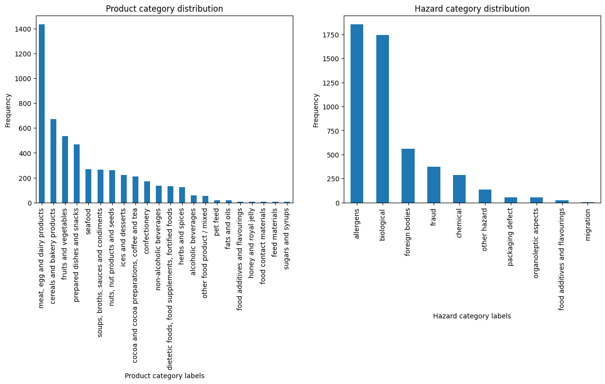
Figure 4: Distributions of hazard-category and product-category for classes occurrences.

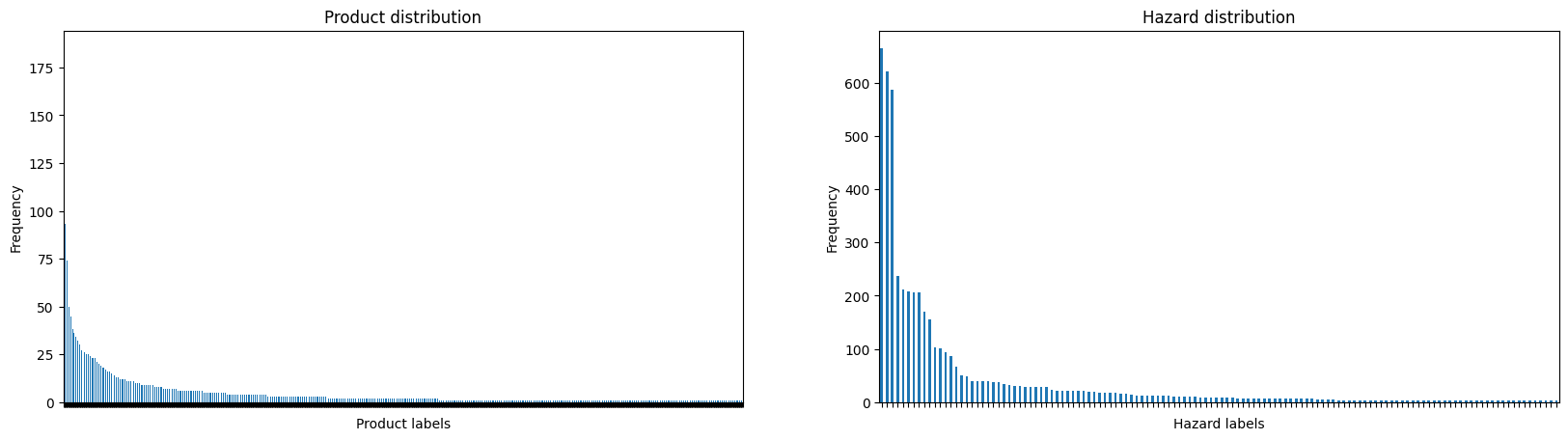
Figure 5: Distributions of hazard and product for classes occurrences. The classes in the x-axis have been omitted due to the large number of classes and clearness of the chart.

The distribution of the four categories’ classes is highly imbalanced, showing a long-tail effect (Figure 4, Figure 5). In coarse categories, 75% of classes have 513 samples in hazard-category and 263 in product-category, while the largest classes contain 1,854 and 1,434 samples, respectively. This imbalance is even more severe in the fine-grained hazard and product classes, with 75% of classes having at most four samples per product and 24 samples per hazard, while the largest class has 185 samples per product and 665 samples per hazard.

4 Methods

We used ML and DL and implemented multiple data augmentation strategies. The next sections describe this in more detail.

4.1 Machine Learning

We used Term Frequency-Inverse Document Frequency (TF-IDF) Sparck Jones (1972) representation of text as input to our ML classifiers. We trained different classifiers and evaluated their performance on both subtasks for each category. The classifiers used were Linear Support Vector Machine (SVM), Decision Tree (DT), Random Forest (RF), Logistic Regression (LR), Multinomial Naive Bayes (NB), and K-Nearest Neighbors (KNN). We used the implementation from Scikit-learn library.

4.2 Deep learning

We used deep learning-based transformer language models for sequence classification Vaswani et al. (2023). We chose encoder-only models that directly produce an input sequence’s representation, which is fed into a classification head to make predictions. We trained various transformers for a sequence classification task, including BERT Devlin et al. (2019), RoBERTa Liu et al. (2019), DistilBERT Sanh et al. (2020), and ModernBERT Warner et al. (2024) (see subsection A.4 for more details). We leveraged the Hugging Face’s Transformers library Wolf et al. (2020).

4.3 Data augmentation on minority classes

In addition to baseline training of the aforementioned models, we explored how data augmentation affected the performance of minority classes for each category.

We employed three different augmentation strategies using the NLP AUG library Ma (2019): random word swapping (RW), synonym replacement (SR), and insertion of contextual words (CW). RW swapping randomly swaps adjacent words. SR substitutes similar words from a lexical database for the English language (WordNet Miller (1995)). CW uses contextual word embeddings from BERT to find the top similar words and insert them for augmentation. An example of each technique applied to a title is shown in Table 1.

Operation	Sentence
Original	Certain Stella Artois brand Beer may be unsafe due to possible presence of glass particles
CW	certain notable stella by artois brand beer may be judged unsafe primarily due to his possible presence of glass particles
SR	Certain Frank stella Artois brand Beer may be insecure imputable to potential presence of glass particles
RW	Certain Stella Artois brand Beer may due be unsafe to presence possible of glass particles

Table 1: Examples of text augmentation techniques applied to a title of a food recall using contextual word insertion (CW), synonym replacement (SR), and random word swapping (RW).

For each strategy, we generated new samples in the training data for minority classes per category by altering titles and texts to preserve their inherent meaning while maintaining the annotated classes. For coarse categories (hazard-category and product-category), we augmented classes with fewer than 200 samples by generating 200 samples for each class. For fine-grained categories (hazard and product), we created 100 samples for classes with fewer than 100 samples for the hazard category and 50 samples for the product category. After examining the entire class distributions, we chose these numbers of added samples and thresholds for low-support classes because they reflect a compromise between improving the representation of minority classes and maintaining low computational costs, but not completely resolving the imbalance issue. We first iterated through the existing data samples for each under-represented class of each category. We then distributed the specified total number of augmentation samples proportionally across these samples (adjusting the final one to ensure the addition matches the set target number of samples to add) to generate new samples based on the augmentation technique used. A pseudocode description is provided in subsection A.5 and its impact on class statistics is provided in subsection A.6. All methods were implemented in Python.

5 Experiments

In the next subsections, we further describe the preprocessing, hyperparameter fine-tuning, and evaluation details.

5.1 Preprocessing

Preprocessing included removal of HTML markup and special characters (newlines, tabs, Unicode character symbols) using regular expressions from title and text and text normalization such as whitespace standardization. This preserves semantic content while eliminating and filtering unnecessary formatting.

5.2 Hyperparameter fine-tuning

We fine-tuned the hyperparameters of baseline and augmented models on the development set using the Tree-structured Parzen Estimator (TPE) sampler in the Optuna hyperparameter optimization framework (Akiba et al., 2019). TPE is a Bayesian-based optimization approach that uses a tree structure to link between the hyperparameters and our objective function (maximizing $F_{1}$-macro score per category) to discover the optimal hyperparameters.

We ran ten trials per model and for each augmentation technique. For the ML for ST1, we ran 50 trials since the computation time was low. We optimized the parameters of the TF-IDF vectorizer, such as the minimum document frequency ($min\_df$), and hyperparameters applicable to each classifier for ML, such as the maximum number of iterations ($max\_iter$) in SVM, and the learning rate scheduler, batch size, and epochs for DL (subsection A.8). All experiments involving transformer models were conducted on different GPU clusters (subsection A.3).

5.3 Evaluation on leaderboard

We submitted our results to the leaderboard for both subtasks, which calculated the final score by averaging the hazard $F_{1}$-macro (computed on all samples) with the product $F_{1}$-macro (computed only on samples with correct hazard predictions) for the coarse (ST1) and fine-grained categories (ST2). For example, if all hazards were predicted correctly, but all products were predicted incorrectly, the overall result would be a 0.5 $F_{1}$-macro score (subsection A.7).

6 Results

The next subsections show quantitative results for each model in the official test set using the text field (trained in training and development sets) and an error analysis on the BERT baseline model versus its augmented-trained versions.

Model hazard-category product-category hazard product ST1 ST2 $SVM_{base}$ 0.701 0.626 0.544 0.234 0.682 0.396 $SVM_{CW}$ 0.655 0.642 0.519 0.256 0.649 0.396 $SVM_{SR}$ 0.707 0.674 0.511 0.234 0.693 0.379 $SVM_{RW}$ 0.687 0.643 0.542 0.246 0.682 0.401 $LR_{base}$ 0.666 0.665 0.511 0.203 0.680 0.368 $LR_{CW}$ 0.713 0.682 0.457 0.209 0.702 0.347 $LR_{SR}$ 0.698 0.677 0.454 0.233 0.691 0.354 $LR_{RW}$ 0.666 0.676 0.522 0.216 0.673 0.380 $DT_{base}$ 0.542 0.445 0.405 0.012 0.484 0.208 $DT_{CW}$ 0.617 0.491 0.427 0.029 0.544 0.230 $DT_{SR}$ 0.576 0.488 0.464 0.037 0.526 0.252 $DT_{RW}$ 0.612 0.475 0.506 0.056 0.542 0.283 $RF_{base}$ 0.691 0.523 0.499 0.129 0.609 0.318 $RF_{CW}$ 0.708 0.597 0.566 0.169 0.642 0.380 $RF_{SR}$ 0.688 0.578 0.455 0.188 0.633 0.331 $RF_{RW}$ 0.698 0.546 0.567 0.202 0.612 0.397 $KNN_{base}$ 0.552 0.497 0.384 0.157 0.527 0.294 $KNN_{CW}$ 0.565 0.490 0.376 0.169 0.534 0.309 $KNN_{SR}$ 0.552 0.507 0.389 0.163 0.537 0.305 $KNN_{RW}$ 0.500 0.491 0.397 0.152 0.515 0.299 $NB_{base}$ 0.553 0.570 0.306 0.064 0.568 0.203 $NB_{CW}$ 0.599 0.586 0.405 0.175 0.603 0.310 $NB_{SR}$ 0.588 0.574 0.444 0.140 0.589 0.314 $NB_{RW}$ 0.603 0.617 0.383 0.167 0.631 0.300 $BERT_{base}$ 0.747 0.757 0.581 0.170 0.753 0.382 $BERT_{CW}$ 0.760 0.761 0.671 0.280 0.762 0.491 $BERT_{SR}$ 0.770 0.754 0.666 0.275 0.764 0.478 $BERT_{RW}$ 0.752 0.757 0.651 0.275 0.756 0.467 $DistilBERT_{base}$ 0.761 0.757 0.593 0.154 0.760 0.378 $DistilBERT_{CW}$ 0.766 0.753 0.635 0.246 0.763 0.449 $DistilBERT_{SR}$ 0.756 0.759 0.644 0.240 0.763 0.448 $DistilBERT_{RW}$ 0.749 0.747 0.647 0.261 0.753 0.462 $RoBERTa_{base}$ 0.760 0.753 0.579 0.123 0.755 0.356 $RoBERTa_{CW}$ 0.773 0.739 0.630 0.000 0.760 0.315 $RoBERTa_{SR}$ 0.777 0.755 0.637 0.000 0.767 0.319 $RoBERTa_{RW}$ 0.757 0.611 0.615 0.000 0.686 0.308 $ModernBERT_{base}$ 0.781 0.745 0.667 0.275 0.769 0.485 $ModernBERT_{CW}$ 0.761 0.712 0.609 0.252 0.741 0.441 $ModernBERT_{SR}$ 0.790 0.728 0.591 0.253 0.761 0.434 $ModernBERT_{RW}$ 0.761 0.751 0.629 0.237 0.759 0.440

Table 2: $F_{1}$-macro scores for each model in the official test set given by the organizers utilizing the text field per category and subtasks scores (ST1 and ST2) rounded to 3 decimals. With bold, we indicated the higher score per category and subtask score.

6.1 Quantitative results

Transformer models outperformed ML across all categories, as shown in Table 2, with the $ModernBERT_{base}$ leading across transformer models, in the baseline version, in all categories except product-category.

Among ML, SVM, LR, and RF showed competitive performance: $LR_{CW}$ scored highest in hazard-category (0.713) and product-category (0.682); $RF_{RW}$ in hazard (0.567), and $SVM_{CW}$ in product (0.256). Among the transformer models, $ModernBERT_{SR}$ scored highest in the hazard-category with a score of 0.790, while $BERT_{CW}$ scored highest in other categories. Augmentation increased performance but was not consistent across the categories. It was more pronounced in ST2 categories than ST1 categories, with the largest score increase (0.11) between $BERT_{base}$ and $BERT_{CW}$ augmentation in the product category.

To understand the impact of augmentation, we conducted individual pairwise Kruskal-Wallis tests comparing the $F_{1}$-macro scores on the $BERT_{base}$ model with the augmented versions, training each version three times per category (Table 9). Statistical significance (P < 0.05) was found in product-category with RW, in hazard with all augmentation techniques, and product with CW and RW (Table 3). This indicates that augmentation techniques for BERT enhanced performance in minority classes more effectively in fine-grained categories than in coarse categories.

We submitted a combination of BERT and RoBERTa models for each category to the leaderboard (subsection B.3), which resulted in an $F_{1}$-macro score of 0.761 for ST1 and of 0.453 for ST2 in the test set. These models were chosen since they indicated the best $F_{1}$-macro scores on the development set. The other models were also evaluated on the test set, but not included in the leaderboard. The best scores achieved on ST1 was 0.769 and ST2 was 0.491, indicated in bold in Table 2.

Moreover, experiments using only title were conducted (where their results can be found in Table 8). We continue with the error analysis on the models using text field since we observed better performance.

Category	CW	RW	SR
hazard-category	0.5127	0.2752	0.2752
product-category	0.2752	0.3758	0.0463
hazard	0.0495	0.0495	0.0463
product	0.0463	0.0495	0.5127

Table 3: Raw P-values from individual pairwise Kruskal-Wallis tests between $BERT_{base}$ model and each of the three augmentation techniques (rounded up to 4 decimals).

6.2 Error Analysis - Confusion Matrices

We investigated the performance and shortcomings on the BERT model, which improved most with the CW technique compared to the baseline.

When comparing the majority and minority classes that were augmented, the $BERT_{CW}$ model predicted the minority classes slightly better than $BERT_{base}$, with a rise from 39 to 41 for hazard-category and from 261 to 277 for hazard (around 6% increase) (Figure 2). However, the model predicted the majority classes slightly worse, decreasing from 656 to 632 for hazard, showing that there is a trade-off between improving the predictions for the minority versus the majority classes. Additionally, while the augmentation slightly improved the prediction of majority classes for the product-category, it decreased the minority class predictions from 106 to 101 samples.

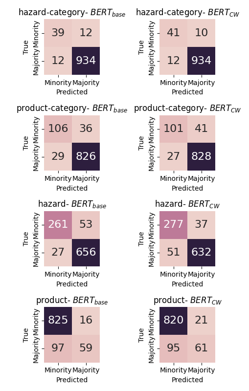
Figure 2: Confusion matrices comparing the performance of the $BERT_{base}$ and $BERT_{CW}$ models in the test set across the four categories showing the changes in the model’s performance for minority and majority class predictions.

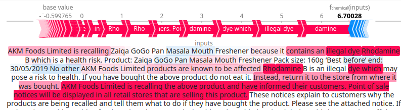
(a) Visualization of a correctly classified sample for hazard-category in baseline model for the true chemical class.

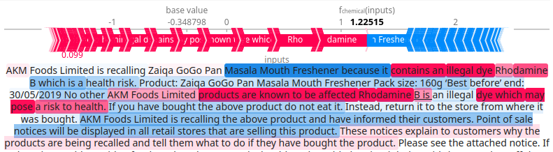
(b) Visualization of a wrongly classified sample for hazard-category in CW augmentation model for the true chemical class.

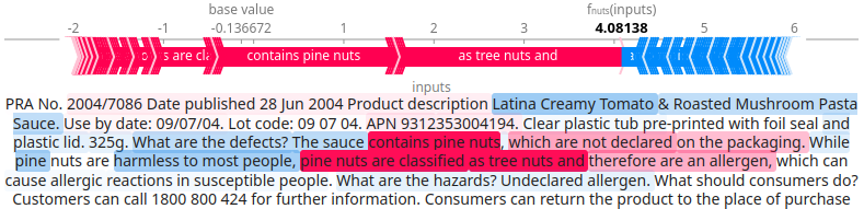
(c) Visualization of a wrongly classified sample for hazard in baseline model for the true nuts class.

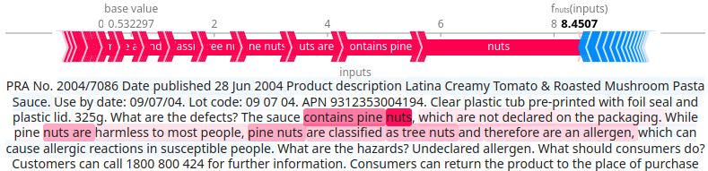
(d) Visualization of a correctly classified sample for hazard in CW augmentation model for the true nuts class.

Figure 3: Visualizations of SHAP values for samples in the ground-truth classes of hazard-category and hazard, based on predictions from the $BERT_{base}$ and $BERT_{CW}$ models. Pink text indicates positive contributions toward predicting this class, while blue text indicates negative contributions. Text which does not contribute in each sample has been truncated.

6.3 Error Analysis - SHAP

We use SHapley Additive exPlanations (SHAP) to further analyze BERT’s prediction behavior. Figures 3(a) and 3(b) illustrate the SHAP values for a sample that was correctly classified with $BERT_{base}$, but was misclassified with $BERT_{CW}$ in the hazard-category, visualizing the contributions for the correct chemical class. Figures 3(c) and 3(d) show the SHAP values for a sample misclassified with $BERT_{base}$ but correctly classified with $BERT_{CW}$ in hazard, visualizing the contributions for the correct nuts class. For the hazard-category, the $BERT_{base}$ correctly identifies features such as ‘illegal dye’ (in pink color), while the CW augmentation has more negative (blue) contributions that push the model’s prediction away from the correct class. For the hazard category, although both models focus on significant terms like ‘pine nuts’, the baseline model focuses on negative contributions like ‘Latina Creamy Tomato’ resulting in a misclassification which may imply that the model associates these features incorrectly with different hazards. This misclassification pattern could serve as a basis for future investigation, further exploring and explaining the model’s predictions to improve its performance and reliability.

7 Limitations

While multiple experiments have been conducted, some limitations could be addressed in future studies. The dataset used was exclusively in English, and the augmentation techniques applied were limited to word-level adjustments. Future research could explore more sophisticated augmentation methods, such as LLMs, to generate new samples and verify their quality. Incorporating datasets in other languages could provide insight into the effectiveness of augmentation techniques. Further investigation could also focus on optimizing the number of augmented samples for minority classes to enhance classification performance, especially for food hazard classification, where reliable models are required to ensure safety. Lastly, to enhance even further the classifiers’ performance, more complex architectures such as ensemble or hierarchical approaches could be used to compare their effectiveness on augmentation in the food hazard classification task.

8 Conclusion

We showed that word-level text augmentation can enhance multi-class classification in minority classes. We used various machine learning and transformer models on the SemEval-2025 Task 9 to assess the effects of these augmentations. Leveraging the text field, we discovered that transformers tend to outperform ML. Augmentation techniques showed a slight increase of $F_{1}$-macro scores, but this effect was not consistent across all augmentations. Comparing $BERT_{base}$ with each augmentation technique, a statistical significant improvement was found for fine-grained categories, which indicates that augmenting minority classes can improve the performance of transformers for these classes.

Appendix A Dataset and Experiments Details

A.1 Dataset Details

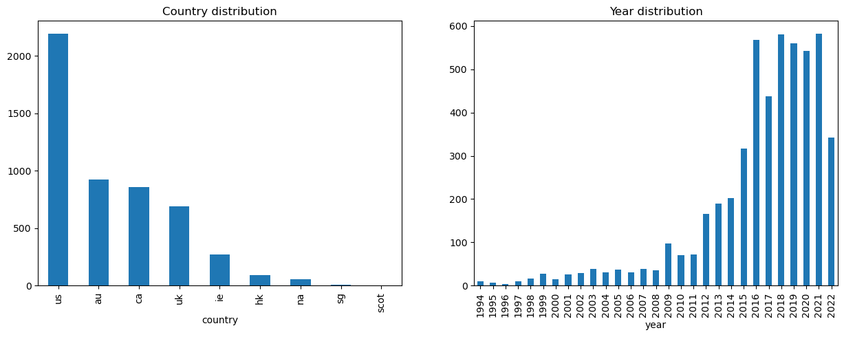
Figure 6: Distributions of occurrences per country (left figure) and per year (right figure) published in the given dataset.

In this section, tables and figures related to the statistics of the provided dataset are presented. Table 11 shows some sample titles and text from the dataset along with their annotated classes. Table 10 presents the number and the names of the annotated classes. Figure 4 and Figure 5 show the distributions of hazard and product classes in coarse and fine-grained categories indicating the long-tail distributions that follow, while Figure 6 presents the distribution of occurrences in the dataset per country and year. Table 4 displays the site domain that the samples have been sourced along their number of samples.

Domain	Samples
www.fda.gov	1740
www.fsis.usda.gov	1112
www.productsafety.gov.au	925
www.food.gov.uk	902
www.lebensmittelwarnung.de	886
www.inspection.gc.ca	864
www.fsai.ie	358
www.foodstandards.gov.au	281
inspection.canada.ca	124
www.cfs.gov.hk	123
recalls-rappels.canada.ca	96
tna.europarchive.org	52
wayback.archive-it.org	23
healthycanadians.gc.ca	18
www.sfa.gov.sg	11
www.collectionscanada.gc.ca	8
securite-alimentaire.public.lu	6
portal.efet.gr	4
www.foodstandards.gov.scot	3
www.ages.at	2
www.accessdata.fda.gov	1
webarchive.nationalarchives.gov.uk	1
www.salute.gov.it	1
www.foedevarestyrelsen.dk	1

Table 4: Data sources of public food safety authority websites, ordered by support number of the given dataset. Table adapted from Randl et al. (2024a). It contains also the sources for the non-English data.

A.2 Preprocessing Dataset Details

The html.parser was leveraged using the BeautifulSoup package to remove the HTML content from the data. The regular expression that was used to remove the special characters is the following:

’[\t\n\r\u200b]|//|&nbsp’

A.3 System Configurations Details

The experiments were run on different machines using Python version 3.10.16. For the fine-tuning and training of transformer models, NVIDIA A100 80GB and NVIDIA GeForce RTX 3070 Ti were utilized. For reproducibility, we used $seed=2025$ as a seed number by employing it in PyTorch, NumPy, and Random packages. To run the BERT model two extra times and calculate the statistical significance, we used $seed=2024$ and $2026$. Moreover, the package versions and their respective URLs that were leveraged can be found in Table 5.

Library	Version	URL
Transformers	4.49.0	https://huggingface.co/docs/transformers/index
PyTorch	2.6.0	https://pytorch.org/
SpaCy	3.8.4	https://spacy.io/
Scikit-learn	1.6.0	https://scikit-learn.org/stable/
Pandas	2.2.3	https://pandas.pydata.org/
Optuna	4.2.1	https://optuna.org/
NumPy	2.0.2	https://numpy.org/
NLP AUG	1.1.11	https://nlpaug.readthedocs.io/en/latest/index.html
BeautifulSoup4	4.12.3	https://www.crummy.com/software/BeautifulSoup/bs4/doc/#

Table 5: Python libraries and their versions with URLs used for the code implementation of the paper.

A.4 Transformer Models Details

In this section, we explain the encoder-only transformer models’ details and architectures we used in the experiments. For BERT Devlin et al. (2019), the bert-base-uncased is used which consists of 110M parameters, 12 encoder layers, a hidden state size of 768, a feed-forward hidden state of 3072, and 12 attention heads, serving as a foundational pre-trained transformer model. For RoBERTa Liu et al. (2019), the roberta-base (case-sensitive) is leveraged and has 125M parameters, structured with 12 encoder layers, a 768-dimensional hidden state, a 3072-dimensional feed-forward network, and 12 attention heads, which is trained on a large corpus leveraging dynamic masking. For DistilBERT Sanh et al. (2020), the distilbert-base-uncased is utilized, which is a lighter BERT variant having 66M parameters and 6 encoder layers while maintaining similar hidden state size and attention heads with BERT. For the ModernBERT Warner et al. (2024), we used the ModernBERT-base (case-sensitive), which contains 149M parameters, 22 encoder layers, hidden state of 768, an intermedia size of 1152, and 12 attention heads. It is trained on 2 trillion tokens, extending the token length to 8192 and incorporating other architectural enhancements to make it faster, lighter, and with better performance than other BERT variants.

A.5 Text Augmentation Details

In Algorithm 1, the function for creating new samples using augmentation is presented. Starting from the inputs of the function, it accepts: a threshold $\tau$ which is the number of samples that a class could contain to be a minority class, the number of samples to add $S$ per minority class, a class counts $C$ that contains the number of samples per class, an augmentation function $F$ that accepts the sample and the number of samples to create, the original training dataset $D$ and the $category$ (e.g. hazard) that we want to augment its classes. The function begins with finding the minority classes by getting the classes with samples less than the given threshold. Then, for each minority class, the respective samples are collected and the number of samples that need to be augmented for each sample is calculated by dividing the total samples over the number of samples of the specific class rounding down the result to the nearest integer. For each sample, then the augmentation function is applied and creates new samples, except for the last sample which is augmented for the remaining number of samples needed. The new samples are inserted into the original training dataset and the function returns the augmented set.

Algorithm 1 Function of creating samples for classification with augmentation

1:Threshold of class number of samples $\tau$, Total samples to add $S$, Class counts $C$, Augmentation function $F$ , Original training dataset $D$, Category to augment $cat$

2:function create_augmented_samples($\tau$, $S$, $C$, $F$, $D$, $cat$)

3:  $minority\_classes\leftarrow\{c\mid C[c]<\tau\}$

4:  $a\_s\leftarrow\emptyset$ $\triangleright$ augmented_samples

5:  for $c$ in $minority\_classes$ do

6:   $samples\leftarrow\{d\in D\mid d[cat]=c\}$

7:   $N\leftarrow\left\lfloor\frac{S}{|\text{samples}|}\right\rfloor$

8:   for $sample$ in $samples$ do

9:     if is the last $sample$ then

10:      $N\leftarrow S-[N*(|samples|-1)]$

11:     end if

12:     $new\_samples\ \leftarrow F(sample,N)$

13:     $a\_s\leftarrow new\_samples\cup\{a\_s\}$

14:   end for

15:  end for

16:  $augmented\_set\leftarrow D\cup a\_s$ return $augmented\_set$

17:end function

A.6 Dataset Classes Statistics

In Table 6, a comparison between the classes’ statistics before and after applying augmentation per category is presented. For hazard-category and product-category, the number of samples that have been created are 200 for classes that have under 200 samples. For hazard and product, the number of samples that have been added are 100 and 50, respectively, for classes that have under 100 samples.

Statistic	hazard-category		product-category
	Initial	Augmented	Initial	Augmented
Count	10		22
Mean	508.2	608.2	231.0	349.2
Standard Deviation	702.75	635.57	325.83	270.79
Minimum	3	203	5	205
25%	53.25	253.25	19.25	212.25
50%	210.5	310.5	132.5	260.5
75%	513.5		263.5	333.25
Maximum	1854		1434
Total Samples	5082	6082	5082	7682

Statistic	hazard		product
	Initial	Augmented	Initial	Augmented
Count	128		1022
Mean	39.7	130.33	4.97	54.87
Standard Deviation	102.19	81.14	10.97	9.72
Minimum	3	101	1	51
25%	4	104	1	51
50%	8.5	108	2	52
75%	24.25	122	4	54
Maximum	665		185
Total Samples	5082	16682	5082	56082

Table 6: Comparison between the initial and after augmentation classes’ statistics per category (hazard-category, product-category, hazard, product) in the training dataset.

A.7 $F_{1}$ Macro Evaluation Metric

For both subtasks, the evaluation metric given by the organizers was the $F_{1}$-macro score on the predicted and the annotated classes. The rankings are based on the hazard classes, meaning that if predictions for both hazard and product are correct, it will get a 1.0 score, while if the hazard predictions are correct but for product are wrong, it will score 0.5. The accurate scoring function can be seen in Algorithm 2.

Algorithm 2 Function for computing score for each subtask.

1:hazard true $ht$, product true $pt$, hazard predictions $hp$, product predictions $pp$

2:function compute_score($ht$, $pt$, $hp$, $pp$)

3:  $\textit{$F_{1}$\_hazards}\leftarrow\text{$F_{1}$-macro}(ht,hp)$

4:  $\textit{cm}\leftarrow(hp==ht)$ $\triangleright$ correct_mask

5:  $\textit{$F_{1}$\_products}\leftarrow\text{$F_{1}$-macro}(pt[\textit{cm}],pp[\textit{ccm}])$

6:  return $\frac{1}{2}(\textit{$F_{1}$\_hazards}+\textit{$F_{1}$\_products})$

7:end function

A.8 Hyperparameters Details

To tune the hyperparameters, the Optuna optimization framework was employed, optimizing based on $F_{1}$-macro scores. For the ML models, the TF-IDF vectorizer parameters, such as $min_{df}$, $max\_df$ etc., were optimized, along with specific parameters for each model, such as $max\_iter$ for SVM and LR, and $alpha$ for NB. The utilized hyperparameters for each model, category, and field are presented in Tables˜12, 13, 14, 15, 16 and 17. When the SpaCy tokenizer is used, English stopwords from SpaCy are also removed from the given text. Balanced class weight was used in SVM, LR, RF, and DT models.

For the transformer models, $batch\_size$, $epochs$, and $lr\_scheduler$ were optimized across all model variants over 10 trials. For all models, the learning rate was set at $5.0\mathrm{e}{-5}$, and the maximum token length that the tokenizer can generate was set at $128$, as no significant differences in performance with higher maximum token length were observed. In Tables˜18, 19, 20 and 21, the utilized hyperparameters for each model, category, and field are listed.

The search space for each hyperparameter used during the tuning can be found in Table 7.

Hyperparameter	Search Space
$C$	{0.1, 1, 5, 10}
$max\_iter$	{100, 1000, 5000}
$n\_estimators$	{100, 200, 300}
$max\_depth$ (DT)	{100, 200, 300}
$max\_depth$ (RF)	{100, 1000, 5000}
$max\_features$	{1000, 5000, 10000, 50000}
$n\_neighbors$	{3, 5, 7, 9, 11}
$weights$	{uniform, distance}
$alpha$	{0.01, 0.1, 1, 5}
$analyzer$	{word, char}
$tokenizer$	{-, SpaCy}
$min\_df$	{1, 2, 5}
$max\_df$	{0.1, 0.3, 0.5}
$ngram\_range$	{(1, 1), (1, 2), (1, 3), (1, 4), (1, 5), (2, 3), (2, 4), (2, 5), (3, 5)}
$batch\_size$	{8, 16, 32}
$epochs$	{3, 5, 10}
$lr\_scheduler$	{lin, cos, cosRestarts}

Table 7: Search space for each hyperparameter used in Optuna optimization trials for ML and transformer models. For learning rate schedulers: cos (cosine annealing), cosRestarts (cosine annealing with restarts), and lin (linear).

Appendix B More Results and Explainability Analysis

B.1 Results using title

Model hazard-category product-category hazard product ST1 ST2 $SVM_{base}$ 0.644 0.692 0.436 0.250 0.670 0.363 $SVM_{CW}$ 0.641 0.675 0.402 0.240 0.657 0.343 $SVM_{SR}$ 0.646 0.699 0.435 0.259 0.674 0.364 $SVM_{RW}$ 0.646 0.690 0.432 0.253 0.670 0.372 $LR_{base}$ 0.596 0.695 0.419 0.261 0.636 0.359 $LR_{CW}$ 0.627 0.670 0.428 0.263 0.649 0.361 $LR_{SR}$ 0.612 0.660 0.425 0.234 0.639 0.350 $LR_{RW}$ 0.634 0.647 0.442 0.269 0.644 0.374 $DT_{base}$ 0.491 0.478 0.330 0.036 0.483 0.183 $DT_{CW}$ 0.534 0.541 0.277 0.031 0.553 0.164 $DT_{SR}$ 0.565 0.449 0.349 0.081 0.495 0.226 $DT_{RW}$ 0.513 0.453 0.298 0.057 0.493 0.185 $RF_{base}$ 0.611 0.633 0.420 0.287 0.616 0.369 $RF_{CW}$ 0.592 0.640 0.446 0.232 0.615 0.367 $RF_{SR}$ 0.638 0.527 0.422 0.207 0.590 0.329 $RF_{RW}$ 0.629 0.635 0.372 0.244 0.638 0.328 $KNN_{base}$ 0.519 0.598 0.349 0.187 0.566 0.299 $KNN_{CW}$ 0.554 0.508 0.341 0.167 0.545 0.275 $KNN_{SR}$ 0.541 0.569 0.306 0.152 0.566 0.255 $KNN_{RW}$ 0.536 0.551 0.335 0.174 0.558 0.278 $NB_{base}$ 0.597 0.641 0.366 0.221 0.624 0.318 $NB_{CW}$ 0.588 0.611 0.360 0.185 0.609 0.305 $NB_{SR}$ 0.597 0.593 0.349 0.180 0.600 0.290 $NB_{RW}$ 0.585 0.629 0.390 0.195 0.608 0.315 $BERT_{base}$ 0.668 0.636 0.372 0.177 0.653 0.284 $BERT_{CW}$ 0.654 0.714 0.502 0.249 0.693 0.392 $BERT_{SR}$ 0.650 0.707 0.489 0.259 0.681 0.389 $BERT_{RW}$ 0.670 0.735 0.477 0.250 0.700 0.372 $DistilBERT_{base}$ 0.653 0.579 0.396 0.248 0.613 0.334 $DistilBERT_{CW}$ 0.631 0.725 0.486 0.264 0.687 0.395 $DistilBERT_{SR}$ 0.640 0.695 0.503 0.262 0.667 0.400 $DistilBERT_{RW}$ 0.644 0.701 0.496 0.267 0.672 0.392 $RoBERTa_{base}$ 0.608 0.629 0.384 0.076 0.619 0.246 $RoBERTa_{CW}$ 0.668 0.692 0.460 0.000 0.686 0.230 $RoBERTa_{SR}$ 0.639 0.718 0.471 0.000 0.673 0.236 $RoBERTa_{RW}$ 0.636 0.736 0.479 0.001 0.690 0.240 $ModernBERT_{base}$ 0.586 0.671 0.393 0.275 0.627 0.353 $ModernBERT_{CW}$ 0.649 0.731 0.423 0.266 0.688 0.372 $ModernBERT_{SR}$ 0.616 0.679 0.422 0.254 0.646 0.364 $ModernBERT_{RW}$ 0.641 0.697 0.385 0.263 0.668 0.351

Table 8: $F_{1}$-macro scores in the official test set given by the organizers utilizing the title field per category and subtasks scores (ST1 and ST2) rounding up to 3 decimals. With bold, we indicate the higher score per column.

In Table 8, we present the experimental results on the test set using the title field for both ML and transformer models. As with the results using text, transformer models overall outperformed the ML models, although they were lower than using text. The best models per category are: $BERT_{RW}$ for hazard-category (0.670), $RoBERTa_{RW}$ for product-category (0.736), $DistilBERT_{SR}$ for hazard (0.503), and $RF_{base}$ for product (0.287). Among the ML models, SVM, LR, and RF demonstrated competitive performance across the categories, similar to the performance observed using only the text field. While there was variability between the baseline and augmented models, a slight, consistent increase was observed in product-category and hazard when using transformer models.

B.2 Statistical Significance Experiments

The mean $F_{1}$-macro scores for the BERT model experiments (both baseline and augmented versions, each run three times) are presented in Table 9.

Model	hazard-category	product-category	hazard	product
$BERT_{base}$	$0.757$	$0.769$	$0.594$	$0.186$
$BERT_{CW}$	$0.768$	$0.756$	$0.658$	$0.284$
$BERT_{RW}$	$0.751$	$0.752$	$0.662$	$0.256$
$BERT_{SR}$	$0.771$	$0.75$	$0.652$	$0.189$

Table 9: Mean $F_{1}$-macro scores per category for each $BERT_{base}$ and with augmentation models running three times using as random seed numbers: 2024, 2025, and 2026.

B.3 Official Submitted Models

Since only one submission was allowed during the evaluation phase, the predictions of the models that were submitted and were found to have the best $F_{1}$-macro scores on the development set for each category are: $RoBERTa_{base}$ for hazard-category with 0.880 $F_{1}$-macro score, $RoBERTa_{RW}$ for product-category with 0.750 $F_{1}$-macro score, $BERT_{CW}$ for hazard with 0.682 $F_{1}$-macro score, $BERT_{RW}$ for product with 0.260 $F_{1}$-macro score (all trained in text field). Then, these models were trained in both train and dev sets and provided their predictions on the test set. When submitting this combination of models, an ST1 score of 0.761 and an ST2 score of 0.4529 were achieved, which are our official leaderboard scores.

Category	Number of Classes	Names of Classes
Hazard Category	10	‘allergens’, ‘biological’, ‘foreign bodies‘, ‘fraud’, ’chemical’, ‘other hazard’, ‘packaging defect’, ‘organoleptic aspects’, ‘food additives and flavourings’, ‘migration’
Product Category	22	‘meat, egg and dairy products’, ‘cereals and bakery products’, ‘fruits and vegetables’, ‘prepared dishes and snacks’, ‘seafood’, ‘soups, broths, sauces and condiments’, ‘nuts, nut products and seeds’,‘ices and desserts’,‘cocoa and cocoa preparations’, ‘coffee and tea’,‘confectionery’,‘non-alcoholic beverages’,‘dietetic foods’, ‘food supplements’, ‘fortified foods’,‘herbs and spices’,‘alcoholic beverages’,‘other food product / mixed’,‘pet feed’,‘fats and oils’,‘food additives and flavourings’,‘honey and royal jelly’,‘food contact materials’, ‘feed materials’, ‘sugars and syrups’
Hazard	128	‘listeria monocytogenes’,‘salmonella’,‘milk and products thereof’,‘escherichia coli’,‘peanuts and products thereof’ … ‘dioxins’,‘staphylococcal enterotoxin’,‘dairy products’,‘sulfamethazine unauthorised’,‘paralytic shellfish poisoning (psp) toxins’
Product	1068	‘ice cream’, ’chicken based products’, ‘cakes’, ‘ready to eat - cook meals’, ‘cookies’ … ‘breakfast cereals and products therefor’, ‘dried lilies’, ‘chilled pork ribs’, ‘tortilla chips cheese’, ‘ramen noodles’

Table 10: Names and number of total classes of the four annotated categories. For hazard and product, some classes are ommited. For product, the total number of classes along with the test data is 1,142.

Title	Text	hazard-category	hazard	product-category	product
Wismettac Asian Foods Issues Allergy Alert on Undeclared Wheat and Soy in Dashi Soup Base	Wismettac Asian Foods, Inc., Santa Fe Springs, CA is recalling 17.6 oz packages of Marutomo Dashi Soup Base because they may contain undeclared wheat and soy. … Consumers with questions may contact the company at recall@wismettacusa.com.	allergens	soybeans and products thereof	soups, broths, sauces and condiments	soups
Kader Exports Recalls Frozen Cooked Shrimp Because of Possible Health Risk	Kader Exports, with an abundance of caution, is recalling certain consignments of various sizes of frozen cooked, peeled and deveined shrimp sold in 1lb, 1.5lb., and 2lb. retail bags. … Consumers with questions may contact the company at +91-022-62621004/ +91-022-62621009, Mon-Fri 10:00hrs -16:00hrs GMT+5.5.	biological	salmonella	seafood	shrimps
Recall Notification: FSIS-024-94	Case Number: 024-94 Date Opened: 07/01/1994 … Product: SMOKED CHICKEN SAUSAGE Problem: BACTERIA Description: LISTERIA Total Pounds Recalled: 2,894 Pounds Recovered: 2,894	biological	listeria monocytogenes	meat, egg and dairy products	smoked sausage

Table 11: Samples from the Food Recall Incidents dataset with title, text and the annotated categories.

Hyperparameters for SVM
	hazard-category				product-category
Parameters	baseline	CW	SR	RW	baseline	CW	SR	RW
	title / text	title / text	title / text	title / text	title / text	title / text	title / text	title / text
$C$	5	1	1 / 10	10 / 1	1 / 10	10	1	5 / 10
$max\_iter$	1000 / 5000	5000 / 100	5000	1000 / 100	5000 / 100	1000	5000	100 / 5000
$max\_features$	50000	50000	50000 / 10000	50000 / 5000	50000	50000	50000	50000
$analyzer$	char	word	word / char	char	char / word	char / word	char	char / word
$tokenizer$	-	SpaCy / -	SpaCy / -	-	-	-	-	-
$max\_df$	0.5 / 0.3	0.1	0.5 / 0.3	0.5	0.5 / 0.1	0.1 / 0.5	0.1	0.3 / 0.5
$min\_df$	1 / 5	1 / 2	1	1 / 2	1 / 2	5	2 / 1	5 / 2
$ngram\_range$	(2, 5) / (1, 5)	(1, 3) / (2, 4)	(1, 2) / (3, 5)	(2, 5) / (2, 4)	(1, 5) / (1, 4)	(2, 5) / (1, 3)	(3, 5)	(2, 5) / (1, 3)
	hazard				product
Parameters	baseline	CW	SR	RW	baseline	CW	SR	RW
	title / text	title / text	title / text	title / text	title / text	title / text	title / text	title / text
$C$	5 / 10	1 / 10	5	1 / 5	10	5 / 1	10 / 5	5 / 10
$max\_iter$	1000 / 5000	5000 / 1000	1000 / 5000	1000 / 5000	100 / 1000	1000 / 100	1000	5000 / 1000
$max\_features$	50000	10000 / 50000	50000 / 10000	50000	5000	5000 / 50000	50000	10000 / 50000
$analyzer$	char	char	word	word / char	char / word	char	char	char
$tokenizer$	-	-	-	-	- / SpaCy	-	-	-
$max\_df$	0.5 / 0.1	0.5 / 0.1	0.1 / 0.3	0.3 / 0.5	0.1 / 0.5	0.1	0.3	0.5 / 0.1
$min\_df$	5 / 1	1 / 2	2 / 1	5 / 2	1 / 5	5 / 2	2 / 1	5 / 1
$ngram\_range$	(2, 4) / (2, 5)	(1, 3) / (3, 5)	(1, 3) / (1, 2)	(1, 2) / (2, 4)	(2, 4) / (1, 1)	(2, 5) / (1, 5)	(3, 5) / (1, 4)	(1, 4) / (2, 4)

Table 12: Hyperparameters for SVM model in each category across baseline, CW, SR, RW variants. Parameters for experiments using title and text fields are separated by a slash ( / ). Default scikit-learn $tokenizer$ is used when not specified and $analyzer$ is word.

Hyperparameters for LR
	hazard-category				product-category
Parameters	baseline	CW	SR	RW	baseline	CW	SR	RW
	title / text	title / text	title / text	title / text	title / text	title / text	title / text	title / text
$C$	5 / 10	10	10 / 5	10	10 / 5	5 / 10	10 / 5	10 / 5
$max\_iter$	5000 / 1000	1000 / 100	1000	5000 / 1000	100 / 5000	5000 / 100	5000	100 / 1000
$max\_features$	10000	50000 / 10000	10000 / 50000	50000 / 10000	50000	50000	10000 / 50000	50000
$analyzer$	char / word	word	char	char	char	char	word / char	word
$tokenizer$	-	SpaCy / -	-	-	-	-	-	SpaCy / -
$max\_df$	0.5	0.1 / 0.3	0.5	0.1 / 0.5	0.5 / 0.1	0.1	0.5 / 0.1	0.5 / 0.3
$min\_df$	1 / 5	2	2 / 1	2 / 1	1 / 2	5	5 / 2	5 / 1
$ngram\_range$	(3, 5) / (1, 3)	(1, 3) / (1, 1)	(2, 4) / (3, 5)	(3, 5) / (1, 5)	(3, 5) / (1, 4)	(1, 5) / (2, 5)	(1, 2) / (2, 5)	(1, 4) / (1, 1)
	hazard				product
Parameters	baseline	CW	SR	RW	baseline	CW	SR	RW
	title / text	title / text	title / text	title / text	title / text	title / text	title / text	title / text
$C$	10 / 5	10	10 / 5	5 / 10	10	10 / 5	10 / 5	5 / 10
$max\_iter$	100 / 1000	100 / 5000	100	100 / 5000	1000 / 5000	5000 / 100	1000 / 5000	1000
$max\_features$	10000 / 50000	10000 / 5000	50000 / 5000	50000 / 5000	50000	50000 / 10000	50000 / 5000	50000 / 5000
$analyzer$	char	char	char	char / word	char	word / char	char / word	char
$tokenizer$	-	-	-	- / SpaCy	-	SpaCy / -	- / SpaCy	-
$max\_df$	0.1 / 0.3	0.5 / 0.1	0.5	0.1	0.1 / 0.3	0.3 / 0.1	0.3 / 0.1	0.3 / 0.1
$max\_iter$	100 / 1000	100 / 5000	100	100 / 5000	1000 / 5000	5000 / 100	1000 / 5000	1000
$min\_df$	1	5 / 2	5	1 / 2	1 / 5	1 / 2	1	1 / 2
$ngram\_range$	(2, 4)	(2, 4) / (1, 4)	(1, 4) / (2, 4)	(2, 5) / (1, 1)	(2, 4) / (3, 5)	(1, 1) / (2, 3)	(2, 3) / (1, 1)	(3, 5) / (2, 3)

Table 13: Hyperparameters for LR model in each category across baseline, CW, SR, RW variants. Parameters for experiments using title and text fields are separated by a slash ( / ). Default scikit-learn $tokenizer$ is used when not specified and $analyzer$ is word.

Hyperparameters for DT
	hazard-category				product-category
Parameters	baseline	CW	SR	RW	baseline	CW	SR	RW
	title / text	title / text	title / text	title / text	title / text	title / text	title / text	title / text
$max\_depth$	100 / 300	100 / 200	300 / 100	200 / 100	100	200 / 100	100 / 300	200 / 300
$max\_features$	5000 / 50000	5000 / 50000	50000	50000 / 10000	50000 / 10000	50000	10000	10000 / 5000
$analyzer$	word / char	word	word / char	word	char / word	word	char / word	word
$tokenizer$	SpaCy / -	SpaCy	-	-	-	SpaCy / -	- / SpaCy	-
$max\_df$	0.5 / 0.1	0.5	0.1 / 0.3	0.1	0.1 / 0.5	0.1	0.3 / 0.1	0.1
$min\_df$	5 / 1	5	1 / 5	1	1	5 / 2	1 / 2	5 / 1
$ngram\_range$	(1, 3) / (2, 5)	(1, 4) / (1, 5)	(1, 3) / (2, 5)	(1, 4) / (1, 1)	(1, 4) / (1, 5)	(1, 4) / (1, 5)	(2, 4) / (1, 2)	(1, 4) / (1, 2)
	hazard				product
Parameters	baseline	CW	SR	RW	baseline	CW	SR	RW
	title / text	title / text	title / text	title / text	title / text	title / text	title / text	title / text
$max\_depth$	300 / 100	200 / 300	200	200	300	100 / 300	200	200 / 300
$max\_features$	50000 / 5000	5000	5000 / 10000	1000 / 50000	50000	1000	1000	1000
$analyzer$	char / word	char / word	word	word	word	char / word	char	word / char
$tokenizer$	-	- / SpaCy	-	- / SpaCy	- / SpaCy	- / SpaCy	-	SpaCy / -
$max\_df$	0.5 / 0.3	0.1 / 0.5	0.1 / 0.3	0.3	0.1	0.5 / 0.1	0.5 / 0.1	0.3 / 0.1
$min\_df$	2 / 5	2	1 / 5	2	5 / 1	2 / 5	2 / 1	2 / 5
$ngram\_range$	(3, 5) / (1, 1)	(1, 5) / (1, 2)	(1, 2) / (1, 1)	(1, 5)	(1, 1) / (2, 3)	(2, 3)	(2, 3) / (2, 5)	(1, 4) / (2, 5)

Table 14: Hyperparameters for DT model in each category across baseline, CW, SR, RW variants. Parameters for title and text fields are separated by a slash ( / ) unless they are the same. Default scikit-learn $tokenizer$ is used when not specified and $analyzer$ is word.

Hyperparameters for RF
	hazard-category				product-category
Parameters	baseline	CW	SR	RW	baseline	CW	SR	RW
	title / text	title / text	title / text	title / text	title / text	title / text	title / text	title / text
$max\_depth$	5000 / 100	100 / 1000	5000 / 100	5000 / 1000	1000 / 100	5000 / 1000	1000 / 100	1000 / 100
$n\_estimators$	100 / 300	100	200	300 / 200	300	300	200	200 / 300
$max\_features$	10000 / 50000	10000 / 50000	10000 / 50000	50000	50000 / 10000	10000 / 50000	10000	50000
$analyzer$	char	word / char	char	char	word	word / char	word	word
$tokenizer$	-	-	-	-	SpaCy	SpaCy / -	-	SpaCy
$max\_df$	0.3	0.1 / 0.3	0.1	0.1 / 0.3	0.1 / 0.3	0.1	0.3 / 0.1	0.1
$min\_df$	2	1	5 / 1	5 / 2	1 / 2	5 / 2	2 / 1	5 / 2
$ngram\_range$	(3, 5) / (2, 5)	(1, 5)	(1, 4) / (1, 5)	(3, 5) / (1, 5)	(1, 2) / (1, 1)	(1, 2) / (1, 5)	(1, 5) / (1, 1)	(1, 2) / (1, 3)
	hazard				product
Parameters	baseline	CW	SR	RW	baseline	CW	SR	RW
	title / text	title / text	title / text	title / text	title / text	title / text	title / text	title / text
$max\_depth$	5000 / 1000	1000	1000 / 100	1000 / 5000	1000	1000	1000	5000 / 1000
$n\_estimators$	300 / 200	300 / 100	200 / 300	200	300	200	200 / 100	300 / 200
$max\_features$	50000	10000 / 50000	5000 / 10000	5000 / 50000	50000 / 10000	50000 / 5000	10000	5000 / 50000
$analyzer$	word / char	char	char	char	char / word	char	word	word
$tokenizer$	SpaCy / -	-	-	-	- / SpaCy	-	SpaCy / -	SpaCy
$max\_df$	0.1	0.5 / 0.1	0.5	0.5 / 0.3	0.3	0.3 / 0.1	0.1	0.3 / 0.1
$min\_df$	2 / 1	2 / 1	5 / 1	2	2 / 5	1 / 5	1 / 5	2 / 1
$ngram\_range$	(1, 2) / (2, 5)	(1, 4) / (1, 5)	(2, 4) / (1, 5)	(1, 5) / (3, 5)	(3, 5) / (1, 4)	(2, 5) / (1, 3)	(1, 1) / (1, 2)	(1, 3) / (1, 1)

Table 15: Hyperparameters for RF model in each category across baseline, CW, SR, RW variants. Parameters for experiments using title and text fields are separated by a slash ( / ). Default scikit-learn $tokenizer$ is used when not specified and $analyzer$ is word.

Hyperparameters for KNN
	hazard-category				product-category
Parameters	baseline	CW	SR	RW	baseline	CW	SR	RW
	title / text	title / text	title / text	title / text	title / text	title / text	title / text	title / text
$n\_neighbors$	3 / 7	7 / 3	11 / 3	5	5	11 / 5	3 / 5	5
$weights$	distance	distance	distance	distance	uniform / distance	distance	distance	distance
$analyzer$	char / word	char / word	char / word	char	word / char	char	char	char
$tokenizer$	-	-	-	-	SpaCy / -	-	-	-
$max\_df$	0.3 / 0.1	0.5 / 0.3	0.5 / 0.3	0.5 / 0.1	0.3 / 0.1	0.3 / 0.1	0.1	0.1
$min\_df$	2 / 5	2	1	5	1	1 / 5	5 / 2	5 / 1
$ngram\_range$	(1, 3) / (1, 4)	(1, 3)	(1, 4)	(2, 3) / (2, 4)	(1, 1) / (3, 5)	(1, 5) / (2, 4)	(1, 4)	(1, 5) / (3, 5)
	hazard				product
Parameters	baseline	CW	SR	RW	baseline	CW	SR	RW
	title / text	title / text	title / text	title / text	title / text	title / text	title / text	title / text
$n\_neighbors$	7	11 / 7	9 / 7	7	3	3	7 / 5	3
$weights$	distance	distance	distance	distance	distance	uniform / distance	distance	uniform
$analyzer$	word / char	char	char	char	char	char	word / char	char
$tokenizer$	-	-	-	-	-	-	-	-
$max\_df$	0.1	0.3	0.3 / 0.1	0.3	0.3 / 0.5	0.5 / 0.1	0.1	0.1 / 0.3
$min\_df$	2 / 5	1	2 / 5	5 / 1	5	1 / 2	5 / 2	2 / 5
$ngram\_range$	(1, 3) / (3, 5)	(2, 5) / (2, 4)	(2, 3) / (2, 4)	(1, 5)	(2, 3) / (1, 5)	(2, 5)	(1, 4) / (2, 5)	(2, 5)

Table 16: Hyperparameters for KNN model in each category across baseline, CW, SR, RW variants. Parameters for experiments using title and text fields are separated by a slash ( / ). Default scikit-learn $tokenizer$ is used when not specified and $analyzer$ is word.

Hyperparameters for NB
	hazard-category				product-category
Parameters	baseline	CW	SR	RW	baseline	CW	SR	RW
	title / text	title / text	title / text	title / text	title / text	title / text	title / text	title / text
$alpha$	0.01	0.01	0.01	0.01	0.01	0.01	0.1 / 0.01	0.1 / 0.01
$analyzer$	word / char	char / word	char / word	word	char	char / word	word / char	word
$tokenizer$	-	-	-	- / SpaCy	-	-	-	SpaCy
$max\_df$	0.1 / 0.5	0.5 / 0.1	0.3 / 0.5	0.1	0.1	0.1 / 0.3	0.1	0.3 / 0.1
$min\_df$	2 / 5	2	1 / 2	1 / 2	2	2	1 / 5	2 / 1
$ngram\_range$	(1, 3) / (2, 5)	(3, 5) / (2, 4)	(1, 4) / (2, 3)	(2, 5) / (1, 3)	(3, 5) / (1, 4)	(2, 5) / (1, 1)	(1, 2) / (3, 5)	(1, 1)
	hazard				product
Parameters	baseline	CW	SR	RW	baseline	CW	SR	RW
	title / text	title / text	title / text	title / text	title / text	title / text	title / text	title / text
$alpha$	0.01	0.01	0.1 / 0.01	0.01	0.01 / 0.1	0.01	0.1	0.1 / 0.01
$analyzer$	char	word	word / char	char	char / word	char	char	word / char
$tokenizer$	-	-	-	-	- / SpaCy	-	-	-
$max\_df$	0.1 / 0.3	0.5 / 0.1	0.5 / 0.1	0.3 / 0.5	0.1 / 0.5	0.3 / 0.1	0.1	0.1
$min\_df$	1 / 5	2	2 / 5	1	5	1	5 / 2	1
$ngram\_range$	(2, 4) / (3, 5)	(1, 1) / (2, 4)	(1, 2) / (1, 5)	(2, 5) / (3, 5)	(2, 5) / (1, 1)	(2, 5) / (2, 4)	(1, 3) / (2, 5)	(1, 1) / (1, 3)

Table 17: Hyperparameters for NB model in each category across baseline, CW, SR, RW variants. Parameters for experiments using title and text fields are separated by a slash ( / ). Default scikit-learn $tokenizer$ is used when not specified and $analyzer$ is word.

Hyperparameters for BERT
	hazard-category				product-category
Parameters	baseline	CW	SR	RW	baseline	CW	SR	RW
	title / text	title / text	title / text	title / text	title / text	title / text	title / text	title / text
$batch\_size$	8 / 32	32 / 16	16 / 8	16 / 32	16 / 8	32 / 8	8 / 32	32
$epochs$	5 / 10	5 / 3	10	3	5 / 10	5	5 / 3	3 / 5
$lr\_scheduler$	cosRestarts / cos	lin	lin	lin / cos	cosRestarts	cosRestarts / lin	cosRestarts / lin	cosRestarts
	hazard				product
Parameters	baseline	CW	SR	RW	baseline	CW	SR	RW
	title / text	title / text	title / text	title / text	title / text	title / text	title / text	title / text
$batch\_size$	16 / 8	16 / 8	16	8	16 / 8	32	32 / 16	32
$epochs$	10	10 / 3	3 / 5	3 / 5	10	3 / 10	5	3 / 5
$lr\_scheduler$	lin / cos	lin / cos	lin	cos / lin	lin	cosRestarts / cos	cos / cosRestarts	lin / cosRestarts

Table 18: Hyperparameters for BERT model in each category across baseline, CW, SR, RW variants. Parameters for experiments using title and text fields are separated by a slash ( / ). Learning rate schedulers: cos (cosine annealing), cosRestarts (cosine annealing with restarts), and lin (linear).

Hyperparameters for RoBERTa
	hazard-category				product-category
Parameters	baseline	CW	SR	RW	baseline	CW	SR	RW
	title / text	title / text	title / text	title / text	title / text	title / text	title / text	title / text
$batch\_size$	8 / 32	16 / 32	8 / 16	32 / 16	32 / 16	8 / 32	32	16
$epochs$	3 / 10	10	10 / 5	10 / 5	5 / 10	3 / 5	3 / 10	10 / 3
$lr\_scheduler$	lin / cos	lin / cosRestarts	cosRestarts / lin	cosRestarts	cosRestarts	lin / cosRestarts	lin	cos
	hazard				product
Parameters	baseline	CW	SR	RW	baseline	CW	SR	RW
	title / text	title / text	title / text	title / text	title / text	title / text	title / text	title / text
$batch\_size$	16	32 / 16	32	16 / 32	16 / 32	16	32	32 / 16
$epochs$	10	10	3	3 / 5	5 / 10	5	5	10
$lr\_scheduler$	lin / cosRestarts	lin	cos / cosRestarts	cos / lin	cosRestarts / cos	cosRestarts / cos	cosRestarts / cos	lin

Table 19: Hyperparameters for RoBERTa model in each category across baseline, CW, SR, RW variants. Parameters for experiments using title and text fields are separated by a slash ( / ). Learning rate schedulers: cos (cosine annealing), cosRestarts (cosine annealing with restarts), and lin (linear).

Hyperparameters for DistilBERT
	hazard-category				product-category
Parameters	baseline	CW	SR	RW	baseline	CW	SR	RW
	title / text	title / text	title / text	title / text	title / text	title / text	title / text	title / text
$batch\_size$	8	32 / 16	16	16 / 8	16 / 8	8	16 / 32	16 / 32
$epochs$	10 / 5	10 / 5	10 / 5	10 / 3	3 / 10	5	5	5 / 3
$lr\_scheduler$	cos	cosRestarts	cos / lin	lin / cosRestarts	lin / cosRestarts	lin	cos / cosRestarts	cos
	hazard				product
Parameters	baseline	CW	SR	RW	baseline	CW	SR	RW
	title / text	title / text	title / text	title / text	title / text	title / text	title / text	title / text
$batch\_size$	8	8 / 16	32	32	8 / 32	32 / 16	16	16 / 32
$epochs$	10	3 / 5	5	3 / 10	10	10	3 / 10	5
$lr\_scheduler$	lin	cos / lin	cosRestarts / cos	lin / cosRestarts	cos / cosRestarts	cos	cosRestarts / lin	lin

Table 20: Hyperparameters for DistilBERT model in each category across baseline, CW, SR, RW variants. Parameters for experiments using title and text fields are separated by a slash ( / ). Learning rate schedulers: cos (cosine annealing), cosRestarts (cosine annealing with restarts), and lin (linear).

Hyperparameters for ModernBERT
	hazard-category				product-category
Parameters	baseline	CW	SR	RW	baseline	CW	SR	RW
	title / text	title / text	title / text	title / text	title / text	title / text	title / text	title / text
$batch\_size$	16 / 8	8 / 32	16	8 / 32	32 / 8	8 / 32	16 / 8	16 / 32
$epochs$	3 / 5	5	5 / 3	10 / 5	5 / 10	5 / 10	5	10
$lr\_scheduler$	cos	cosRestarts / lin	cos / lin	cosRestarts / cos	lin / cos	cos / cosRestarts	cosRestarts / lin	cos / cosRestarts
	hazard				product
Parameters	baseline	CW	SR	RW	baseline	CW	SR	RW
	title / text	title / text	title / text	title / text	title / text	title / text	title / text	title / text
$batch\_size$	32 / 8	16 / 8	8	32 / 8	8	8	8	8
$epochs$	10	5 / 10	5	5	10	5	10 / 5	3
$lr\_scheduler$	cosRestarts / lin	cos / cosRestarts	lin / cosRestarts	cos	cos	cosRestarts	lin / cos	cos

Table 21: Hyperparameters for ModernBERT model in each category across baseline, CW, SR, RW variants. Parameters for experiments using title and text fields are separated by a slash ( / ). Learning rate schedulers: cos (cosine annealing), cosRestarts (cosine annealing with restarts), and lin (linear).

References

- Akiba et al. (2019) Takuya Akiba, Shotaro Sano, Toshihiko Yanase, Takeru Ohta, and Masanori Koyama. 2019. Optuna: A next-generation hyperparameter optimization framework. In Proceedings of the 25th ACM SIGKDD International Conference on Knowledge Discovery and Data Mining.
- Al-Azzawi et al. (2023) Sana Al-Azzawi, György Kovács, Filip Nilsson, Tosin Adewumi, and Marcus Liwicki. 2023. NLP-LTU at SemEval-2023 task 10: The impact of data augmentation and semi-supervised learning techniques on text classification performance on an imbalanced dataset. In Proceedings of the 17th International Workshop on Semantic Evaluation (SemEval-2023), pages 1421–1427, Toronto, Canada. Association for Computational Linguistics.
- Devlin et al. (2019) Jacob Devlin, Ming-Wei Chang, Kenton Lee, and Kristina Toutanova. 2019. BERT: Pre-training of deep bidirectional transformers for language understanding. In Proceedings of the 2019 Conference of the North American Chapter of the Association for Computational Linguistics: Human Language Technologies, Volume 1 (Long and Short Papers), pages 4171–4186, Minneapolis, Minnesota. Association for Computational Linguistics.
- Gopali et al. (2024) Saroj Gopali, Faranak Abri, Akbar Siami Namin, and Keith S. Jones. 2024. The applicability of llms in generating textual samples for analysis of imbalanced datasets. IEEE Access, 12:136451–136465.
- Henning et al. (2023) Sophie Henning, William Beluch, Alexander Fraser, and Annemarie Friedrich. 2023. A survey of methods for addressing class imbalance in deep-learning based natural language processing. In Proceedings of the 17th Conference of the European Chapter of the Association for Computational Linguistics, pages 523–540, Dubrovnik, Croatia. Association for Computational Linguistics.
- Khan and Venugopal (2024) Reeba Khan and Anoushka Venugopal. 2024. Exploring deep learning methods for text augmentation to handle imbalanced datasets in natural language processing. In 2024 3rd Edition of IEEE Delhi Section Flagship Conference (DELCON), pages 1–8.
- Liu et al. (2019) Yinhan Liu, Myle Ott, Naman Goyal, Jingfei Du, Mandar Joshi, Danqi Chen, Omer Levy, Mike Lewis, Luke Zettlemoyer, and Veselin Stoyanov. 2019. Roberta: A robustly optimized bert pretraining approach. Preprint, arXiv:1907.11692.
- Ma (2019) Edward Ma. 2019. Nlp augmentation. https://github.com/makcedward/nlpaug.
- Miller (1995) George A. Miller. 1995. Wordnet: a lexical database for english. Commun. ACM, 38(11):39–41.
- Randl et al. (2024a) Korbinian Randl, Manos Karvounis, George Marinos, John Pavlopoulos, Tony Lindgren, and Aron Henriksson. 2024a. Food recall incidents.
- Randl et al. (2024b) Korbinian Randl, John Pavlopoulos, Aron Henriksson, and Tony Lindgren. 2024b. CICLe: Conformal in-context learning for largescale multi-class food risk classification. In Findings of the Association for Computational Linguistics: ACL 2024, pages 7695–7715, Bangkok, Thailand. Association for Computational Linguistics.
- Randl et al. (2025) Korbinian Randl, John Pavlopoulos, Aron Henriksson, Tony Lindgren, and Juli Bakagianni. 2025. SemEval-2025 task 9: The food hazard detection challenge. In Proceedings of the 19th International Workshop on Semantic Evaluation (SemEval-2025), Vienna, Austria. Association for Computational Linguistics.
- Sanh et al. (2020) Victor Sanh, Lysandre Debut, Julien Chaumond, and Thomas Wolf. 2020. Distilbert, a distilled version of bert: smaller, faster, cheaper and lighter. Preprint, arXiv:1910.01108.
- Shorten et al. (2021) Connor Shorten, Taghi M. Khoshgoftaar, and Borko Furht. 2021. Text data augmentation for deep learning. Journal of Big Data, 8(1):101.
- Sparck Jones (1972) Karen Sparck Jones. 1972. A statistical interpretation of term specificity and its application in retrieval. Journal of Documentation, 28(1):11–21.
- Vaswani et al. (2023) Ashish Vaswani, Noam Shazeer, Niki Parmar, Jakob Uszkoreit, Llion Jones, Aidan N. Gomez, Lukasz Kaiser, and Illia Polosukhin. 2023. Attention is all you need. Preprint, arXiv:1706.03762.
- Warner et al. (2024) Benjamin Warner, Antoine Chaffin, Benjamin Clavié, Orion Weller, Oskar Hallström, Said Taghadouini, Alexis Gallagher, Raja Biswas, Faisal Ladhak, Tom Aarsen, Nathan Cooper, Griffin Adams, Jeremy Howard, and Iacopo Poli. 2024. Smarter, better, faster, longer: A modern bidirectional encoder for fast, memory efficient, and long context finetuning and inference. Preprint, arXiv:2412.13663.
- Wei and Zou (2019) Jason Wei and Kai Zou. 2019. EDA: Easy data augmentation techniques for boosting performance on text classification tasks. In Proceedings of the 2019 Conference on Empirical Methods in Natural Language Processing and the 9th International Joint Conference on Natural Language Processing (EMNLP-IJCNLP), pages 6382–6388, Hong Kong, China. Association for Computational Linguistics.
- Wolf et al. (2020) Thomas Wolf, Lysandre Debut, Victor Sanh, Julien Chaumond, Clement Delangue, Anthony Moi, Pierric Cistac, Tim Rault, Remi Louf, Morgan Funtowicz, Joe Davison, Sam Shleifer, Patrick von Platen, Clara Ma, Yacine Jernite, Julien Plu, Canwen Xu, Teven Le Scao, Sylvain Gugger, Mariama Drame, Quentin Lhoest, and Alexander Rush. 2020. Transformers: State-of-the-art natural language processing. In Proceedings of the 2020 Conference on Empirical Methods in Natural Language Processing: System Demonstrations, pages 38–45, Online. Association for Computational Linguistics.
- World Health Organization (2024) World Health Organization. 2024. Food safety. https://www.who.int/news-room/fact-sheets/detail/food-safety. Accessed: February 03, 2025.