Coupled-wire Construction of a Non-crystalline Fractional Quantum Hall Effect

Abstract

The fractional quantum Hall effect, a paradigmatic topologically ordered state, has been realised in two-dimensional strongly correlated quantum gases and Chern bands of crystals. Here we construct a non-crystalline analogue by coupling quantum wires that are not periodically placed in real-space. Remarkably, the model remains solvable using bosonisation techniques. Due to the non-uniform couplings between the wires, the ground state has different degeneracy compared to the crystalline case. It displays a rich phenomenology of excitations, which can either behave like anyons confined to move in one dimension (lineons), anyons confined to hop between two wires (s-lineons), and anyonic excitations that are free to travel across the system. Both the ground state degeneracy and mutual statistics are directly determined by the real-space positions of the wires. By providing an analytically solvable model of a non-crystalline fractional quantum Hall effect, our work showcases that topological order can display richer phenomenology beyond crystals. More broadly, the non-uniform wire construction we develop can serve as a tool to explore richer many-body phenomenology in non-crystalline systems.

I Introduction

Topologically ordered phases encode information non-locally through long-range entanglement, a feature that can be exploited to engineer quantum computers robust to decoherence by braiding the underlying anyon excitations [1, 2]. Hence, finding and classifying topologically ordered phases is a central goal of condensed matter [3].

The search for topological order is often guided by progress in crystalline systems, and builds on our understanding of non-interacting topological phases. As for topological band insulators, topological order was shown to survive until the strength of disorder closes the mobility gap. For example, the plateaus of the fractional quantum Hall effect [4], a paradigmatic example of topological order [5], shrink and disappear for sufficiently strong potential disorder [6] and electric conductance can exhibit mesoscopic fluctuations [7, 8, 9, 10, 11]. This would suggest that looking for topological order in a non-crystalline system is not a fruitful strategy.

However, there are several examples where strong disorder is not detrimental, and can even be beneficial, for topological order. For instance, the toric code ground state [1], another topologically ordered state, can be defined in any four-fold coordinated graph [1, 12]. It is also possible to define fractional quantum Hall states with trial wave-functions on non-crystalline lattices, for example in fractals [13, 14, 15, 16, 17, 18] and quasicrystals [19].

More strikingly, disorder or non-crystallinity can help to tune into and control the properties of a topologically ordered state. For example, moiré heterostructures, lacking strict lattice periodicity, allow topological bands to flatten by rotating two monolayer materials with respect to one another. By exploiting this freedom, recent experiments have reported the anomalous fractional quantum Hall effect in twisted MoTe₂ [20, 21, 22, 23, 24] and rhombohedral multilayer graphene [25, 26, 27, 28], realizing the long-sought prediction of a fractional Hall effect without magnetic fields [29, 30, 31, 32, 33]. Additionally, structural disorder or amorphisation can open a gap in Kitaev’s honeycomb quantum spin-liquid phase leading to a topological, non-abelian chiral spin-liquid phase [34, 35]. This success motivates the question we address in this work.

While non-crystalline systems can realise topological order, can we go further and exploit non-crystallinity to define topologically ordered states with different features compared to their crystalline counterparts? Recent advances in non-crystalline, single particle topological states, which have been defined in several non-crystalline settings, including quasicrystals [36, 37, 38, 39, 40, 41, 42, 43, 44, 45, 19, 46, 47, 48, 49], amorphous systems [50, 51, 52, 53, 54, 55, 56, 57, 58, 59, 60, 61, 62, 63, 64, 65, 66, 67, 68, 69, 70, 71, 72, 73, 74, 75, 76, 35, 34, 77, 78, 79] and fractals [80, 81, 82, 83, 84, 85, 86, 87, 88, 89, 90, 91, 92, 93, 94, 95, 96, 97], suggest that this can indeed be the case.

The goal of this paper is to propose a solvable model for a non-crystalline fractional quantum Hall phase with different properties compared to its crystalline counterpart. This is done using a system of coupled one-dimensional wires, a successful strategy for constructing solvable fractionalised topologically ordered phases [98, 99, 100, 101, 102, 103, 104, 105, 106].

The coupled-wire construction has been used to construct a rich variety of anisotropic, yet still crystalline, many-body states. These include fractionalised topological phases [107, 108, 109, 110, 111, 112, 113, 114, 115, 116, 117, 118, 119, 120, 121, 122, 123, 124, 125, 126, 127, 128, 129, 130, 131, 132, 133, 134, 104, 135, 136, 137, 138], spin liquids [139, 140, 141, 142, 143, 144, 145, 146, 147, 148] and fractonic states [149, 150, 151, 152, 153, 154]. More recently, the wire construction has also allowed us to analytically describe strongly correlated topological states in twisted moiré heterostructures, as a network of crossing coupled wires [155, 156, 157, 158, 159, 160, 161, 162, 163].

Despite its success, the wire construction has been exclusively used to describe crystalline phases. A possible reason is that the couplings necessary for a fractionalised phase must be precisely chosen to satisfy charge and momentum conservation, while still retaining exact solubility. This places strong constraints on the arrangement of the wires and generally forbids disordered configurations from admitting an exact solution under bosonisation. One might then worry that any model with non-uniform spacing between the wires becomes unsolvable.

Here we show that this is not the case. By considering coupled wires whose real space configuration is disordered and non-uniform, shown in Fig. 1a, we show that the problem remains solvable via bosonisation. We formalise the constraints on the disordered couplings under which the bosonic fields commute among themselves, while also conserving charge and momentum—thus retaining exact solvability. This problem is equivalent to that of gapping out fractional quantum Hall edge states [9, 164, 165], depicted in Fig. 1b, providing a pathway to realise these novel properties by coupling fractional quantum Hall edges.

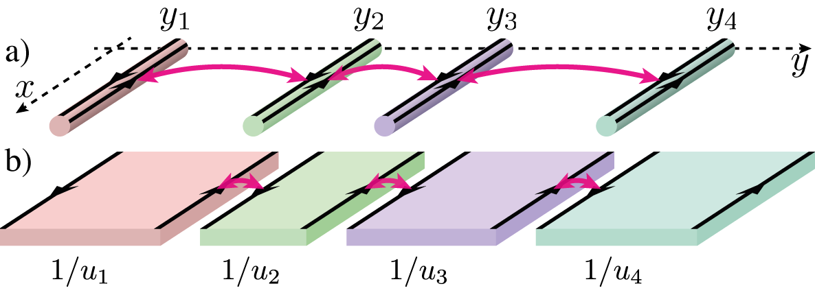
Figure 1: The mapping from (a) non-uniformly coupled wires to (b) coupled Hall droplets. Wires are placed at a set of (non-uniformly spaced) positions $\{y_{j}\}$ and coupled together to form a non-uniform fractional Hall phase. Couplings depend on the inter-wire separation, and so are themselves non-uniform. The left- and right-movers on each differently fractionalised wire can be mapped onto the left- and right-moving edge modes in each fractional Hall droplet. The couplings necessary to gap out the non-uniform arrangement of wires in (a) are identical to the couplings necessary to gap out the fractionalised gapless edge modes of adjacent fractional quantum Hall droplets in (b).

We show that the non-crystalline fractional quantum Hall states constructed in this way display features different from their crystalline counterparts. Specifically, we find distinct ground state degeneracy and anyon properties, which depend on the real-space arrangement of the wires. The zoology of anyons includes three types of fractionalised excitations: an excitation constrained to move along the wires (known as lineon in the fractonic language), a composite particle only able to travel up to the next wire and back (which we call a spread-lineon or s-lineon for short), and a composite anyon with complete freedom to travel throughout the system, which we refer to as a C-anyon. Their mutual statistics depends on the real-space arrangement of the wires, that differ in general compared to the crystalline case.

The outline of this paper is as follows: In Section II we lay the foundations for our model, defining the wire construction and its reformulation in terms of bosonised operators. In Section III we show how the degrees of freedom in a single wire may be re-expressed in a basis of fractionalised bosonic operators. Next, we show how couplings may be introduced between adjacent wires that gap out these fractionalised excitations, thus allowing the wires to host a single correlated phase of matter. Importantly, we see that it is possible to couple two adjacent wires even when each hosts differently fractionalised excitations, and discuss the conditions under which this coupling preserves exact solvability and is gapped. Finally, in Section IV we show how this constitutes a general construction of composite and disordered fractional phases, created by gluing many regions with different fractionalisation together. We determine the ground state degeneracy of such a composite system and study the properties of the quasiparticles (both fractonic and non-fractonic) that emerge, determining their charge and braiding statistics.

II The Model

We start by introducing the model, which will follow a familiar procedure to Refs. [102, 103, 104]. We construct an array of coupled fermionic wires, aligned in the $x$-direction, with the $j^{\textup{th}}$ wire placed at position $y_{j}$. Penetrating the plane is a magnetic field $B$, which we represent in the Landau gauge, $\textbf{A}=-By\hat{\textbf{x}}$. On each wire sits a single species of fermion, represented with the creation operators $\psi_{j}(x)$ that satisfy

$$\{\psi_{j}^{\dagger}(x),\psi_{k}^{\phantom{{\dagger}}}(x^{\prime})\}=2\pi\delta_{jk}\delta(x-x^{\prime}).$$ (1)

The Hamiltonian for each uncoupled wire is given by

$$H_{j}=\int\frac{\mathrm{d}x}{2\pi}\psi_{j}^{\dagger}(x)\frac{\left(-i\partial_{x}-By_{j}\right)^{2}}{2m}\psi_{j}^{\phantom{{\dagger}}}(x),$$ (2)

which leads to a parabolic dispersion for the fermions on each wire, with the parabola shifted according to the wire’s position, $E_{j}(k)=\left(k-By_{j}\right)^{2}/2m$. We impose a global Fermi level and corresponding Fermi momentum, $E_{F}=k_{F}/2m$, such that in each wire all momentum states that satisfy $|k_{j}-By_{j}|\leq k_{F}$ are filled, as shown in Fig. 2a.

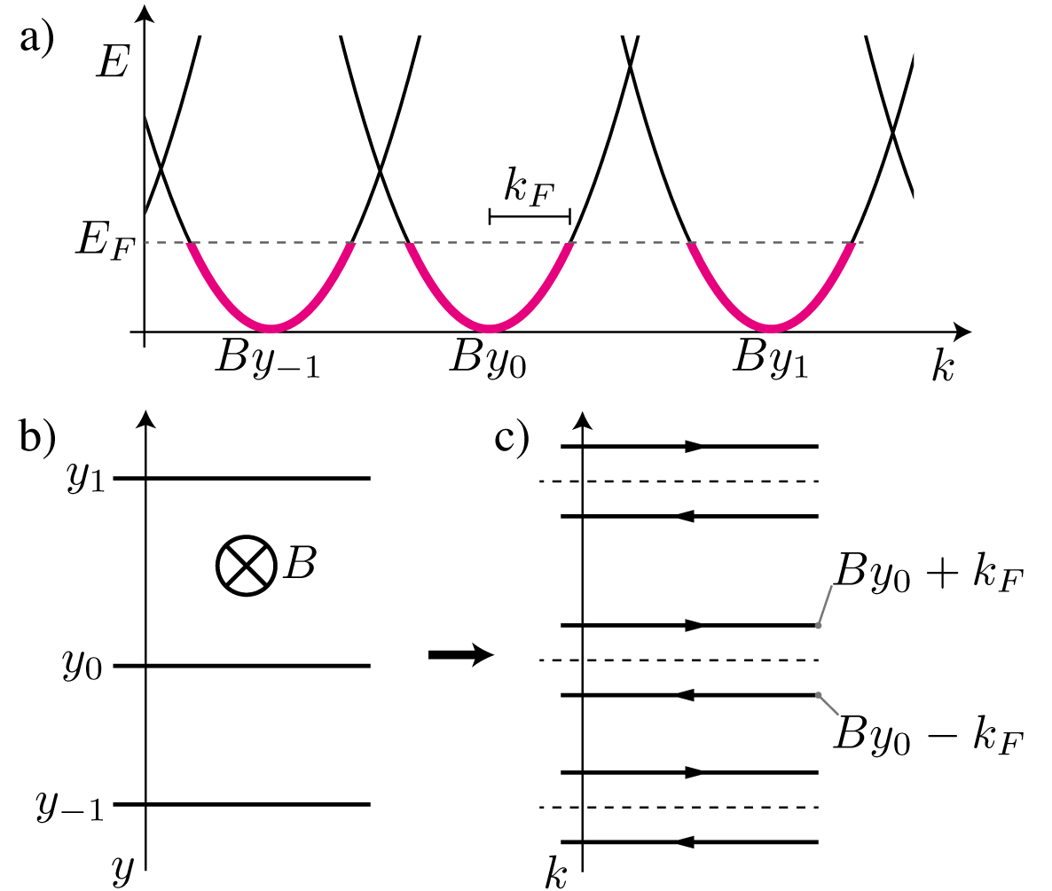
Figure 2: (a) Dispersion for three coupled wires placed at positions $y_{j}$ in a field $B$. Filled states are highlighted in magenta and the Fermi momentum is labelled with $k_{F}$. Note that wires here are not regularly spaced, so the centres of the parabolas are also not evenly spaced. (b) Real space diagram showing the positions of each wire, and the orientation of the applied field. (c) The low-energy spectrum of each wire is effectively split into a set of left movers and right movers, shifted from the central $k$ of each wire by $k_{F}$. Dashed lines indicate the values of $By_{j}$.

For a given Fermi level, the low-energy, long-wavelength properties of the system are defined only by the electrons close to $E_{F}$. Thus, we may construct an effective description by linearising the dispersion relation around these points. On each wire, the $\psi_{j}(x)$ fermion can be decomposed into a pair of $\psi^{R}_{j}(x)$ and $\psi^{L}_{j}(x)$ fermions, corresponding to right-movers and left-movers, by separating positive and negative momentum states. We thus derive the linearised Hamiltonian for a given wire as

$$H_{j}^{\textup{Lin}} =H_{j}^{R}+H_{j}^{L},$$ (3)

$$H_{j}^{R} =\int\frac{\mathrm{d}x}{2\pi}v{\psi^{R}_{j}}^{\dagger}(x)(-i\partial_{x}){\psi^{R}_{j}}^{\phantom{{\dagger}}}(x),$$ (4)

$$H_{j}^{L} =\int\frac{\mathrm{d}x}{2\pi}v{\psi^{L}_{j}}^{\dagger}(x)(i\partial_{x}){\psi^{L}_{j}}^{\phantom{{\dagger}}}(x),$$ (5)

with $v=\frac{k_{F}}{m}$. Each wire is effectively split into a pair of wires, each with unidirectional transport at a pair of momenta shifted by $\pm k_{F}$, as shown in Fig. 2b. Note that Eqs. 5 and 4 should include a shift by the momentum at the Fermi level, $k_{j}^{p}=y_{j}B+(-1)^{p}k_{F}$, where $p\in\{R,L\}$. This shift is removed by redefining $\psi^{a}_{j}(x)\rightarrow e^{ik_{j}^{p}x}\psi^{a}_{j}(x)$.

II.1 Allowed Couplings

To realise an effective 2D phase, we must now introduce couplings between adjacent wires. A general coupling is expressed in terms of a set of parameters $s_{j}^{R}$ and $s_{j}^{L}$, that denote the number of right and left-movers created respectively on the $j^{\textup{th}}$ wire. Such a coupling may be written as

$$\mathcal{O}_{\{s_{j}\}}(x)\propto\prod_{j}{\psi^{R}_{j}}^{(s_{j}^{R})}(x){\psi^{L}_{j}}^{(s_{j}^{L})}(x)+h.c.,$$ (6)

where we write ${\psi^{a}_{j}}^{\dagger}$ when $s_{j}^{p}>0$. Since fermionic operators square to zero, these terms must be written using a point-splitting prescription [166]. The coupling Hamiltonian is expressed as a sum over all such coupling terms.

The couplings in Eq. 6 may be represented pictorially as shown in Fig. 3a. It will be convenient to re-express these in terms of two new variables,

$$n_{j} =s_{j}^{R}+s_{j}^{L},$$ (7)

$$m_{j} =s_{j}^{R}-s_{j}^{L},$$ (8)

where $n_{j}$ is the total number of fermions arriving at or leaving the wire, and $m_{j}$ encodes the transfer of fermions from $L$ to $R$ on a given wire. Note that $n_{j}$ and $m_{j}$ can take any value so long as both are even or both are odd,

$$m_{j}=n_{j}\mod 2.$$ (9)

Such couplings must generally satisfy charge and momentum conservation. To conserve charge, couplings must not produce a net change in the overall number of fermions,

$$\sum_{j}n_{j}=0,$$ (10)

whereas to conserve momentum we require that

$$\sum_{j}By_{j}n_{j}+k_{F}m_{j}=0.$$ (11)

We have freedom to choose the position of each wire, $y_{j}$. For a desired coupling between a set of $a$ wires we have two constraints and $a$ degrees of freedom. Thus, provided the coupling satisfies charge conservation, it is always possible to choose values of $\{y_{j}\}$ such that momentum is conserved. Every coupling thus implies a set of positions (or family of positions for $a>2$) for which this coupling conserves momentum. Thus, constructing an irregular array of wires necessitates irregular, spatially dependent couplings between wires.

II.2 Bosonisation

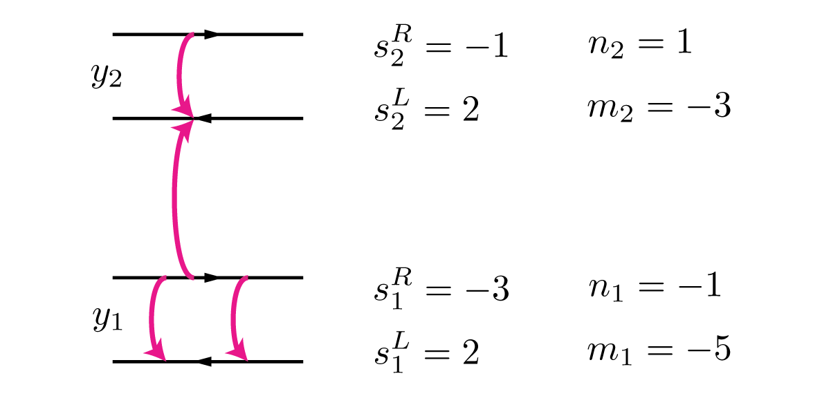
Figure 3: A diagram for an example coupling between two wires, showing left and right movers explicitly. Vertical arrows indicate the transfer of fermions between wires, and the description of the hopping is shown in terms of $s_{j}$, and equivalently in terms of $n/m_{j}$. The $s_{j}$ parameters correspond exactly to the number of left and right fermions arriving on each wire, whereas $n_{j}$ denotes the total number of fermions arriving, and $m_{j}$ denotes the change of occupation from left to right on each wire.

So far, we have constructed a generic Hamiltonian, represented by a set of linearised dispersive terms, $H^{\textup{Lin}}_{j}$, Eq. 3, and some set of couplings $\mathcal{O}_{\{s_{j}\}}(x)$, Eq. (6). The next step is to write down the bosonic reformulation of this system [167, 168, 166]. We primarily use the conventions of Ref. [166], introducing a set of bosonic fields for left and right movers on each wire, $\phi_{j}^{L/R}$, which satisfy the following commutation relations

$$[\partial_{x}\phi_{j}^{p}(x),\phi_{k}^{q}(x^{\prime})]=(-1)^{p}2\pi i\,\delta_{jk}\delta_{pq}\delta(x-x^{\prime}).$$ (12)

We make use of the bosonisation identity to express our system in terms of these operators,

$$\psi^{p}_{j}(x) \propto e^{-i\phi_{j}^{p}(x)},$$ (13)

where we have neglected to include the terms proportional to number density, as well as Klein factors [166, 102, 103]. Furthermore, we use the following two identities for the kinetic term in $H^{\textup{Lin}}_{j}$ and the fermionic number density,

$${\psi^{p}_{j}}^{\dagger}(x)[-i\partial_{x}]\psi^{p}_{j}(x) =(-1)^{p}\frac{1}{2}{(\partial_{x}\phi_{j}^{p}(x))^{2}},$$ (14)

$$\rho^{p}_{j}={\psi^{p}_{j}}^{\dagger}(x)\psi^{p}_{j}(x) =(-1)^{p}\partial_{x}\phi_{j}^{p}.$$ (15)

Thus, the linearised Hamiltonian takes the following bosonic form,

$$H_{j}^{\textup{Lin}}=\int\frac{\mathrm{d}x}{2\pi}\frac{v}{2}\left[\left(\partial_{x}\phi_{j}^{L}(x)\right)^{2}+\left(\partial_{x}\phi_{j}^{R}(x)\right)^{2}\right].$$ (16)

Finally, we can write an arbitrary coupling between wires in terms of the bosonic fields, by combining Eqs. 6 and 13

$$\mathcal{O}_{\{s_{j}\}}(x)\propto\cos\bigg{(}\sum_{j}s_{j}^{L}\phi_{j}^{L}(x)+s_{j}^{R}\phi_{j}^{R}(x)\bigg{)}.$$ (17)

II.2.1 Sum and Difference Fields

Let us define a pair of bosonic sum and difference fields, which will often be more convenient than working in the $\phi^{a}_{j}$ basis,

$$\varphi_{j} =\frac{1}{2}\left(\phi_{j}^{R}(x)+\phi_{j}^{L}(x)\right),$$ (18)

$$\theta_{j} =\frac{1}{2}\left(\phi_{j}^{R}(x)-\phi_{j}^{L}(x)\right),$$ (19)

which satisfy the commutation relations

$$\left[\partial_{x}\theta_{j}(x),\varphi_{k}(x^{\prime})\right] =\pi i\delta_{jk}\delta(x-x^{\prime}),$$ (20)

$$\left[\partial_{x}\theta_{j}(x),\theta_{k}(x^{\prime})\right] =\left[\partial_{x}\varphi_{j}(x),\varphi_{k}(x^{\prime})\right]=0.$$ (21)

In terms of these fields, the linearised Hamiltonian, Eq. 16, takes the form

$$H_{j}^{\textup{Lin}}=\int\frac{\mathrm{d}x}{2\pi}v\left[\left(\partial_{x}\varphi_{j}(x)\right)^{2}+\left(\partial_{x}\theta_{j}(x)\right)^{2}\right],$$ (22)

and each coupling, given by Eq. 17, may be written in terms of the $n_{j}$ and $m_{j}$ variables defined in Eqs. 7 and 8,

$$\mathcal{O}_{\{s_{j}\}}(x)\propto\cos\bigg{(}\sum_{j}n_{j}\varphi_{j}(x)+m_{j}\theta_{j}(x)\bigg{)}.$$ (23)

Let us also consider the total density operator on a given wire,

$$\rho_{j}(x)=L^{\dagger}_{j}(x)L_{j}(x)+R^{\dagger}_{j}(x)R_{j}(x).$$ (24)

Written in terms of bosonic fields, using Eq. 15, this takes the form

$$\begin{aligned} \rho_{j}(x)&=\partial_{x}\phi^{R}(x)-\partial_{x}\phi^{L}(x),\\ &=2\partial_{x}\theta_{j}(x).\end{aligned}$$ (25)

Thus, we see that the variation of $\theta_{j}(x)$ encodes the fermionic density on the $j$^th wire.

III Fractionalisation

In this section, we shall show how the construction above allows us to produce fractionalised fermionic states. First, we will show in Section III.1 how the left and right-moving fermions on a single wire can be re-expressed in terms of a pair of fractionalised quasiparticle fields. By introducing an appropriate coupling between such fields, we then see how one can stabilise a fractionalised phase, where these quasiparticles make up the low-energy excitations. This discussion largely follows Refs. [102, 103]. Then in Section III.2 we show how it is possible to construct composite materials by connecting wires with different fractionalisation. Crucially, we will see that it is possible to introduce couplings that can gap out left edge modes from one wire with right edge modes from another, where the two wires are fractionalised differently.

III.1 Uniform Fractionalised Phases

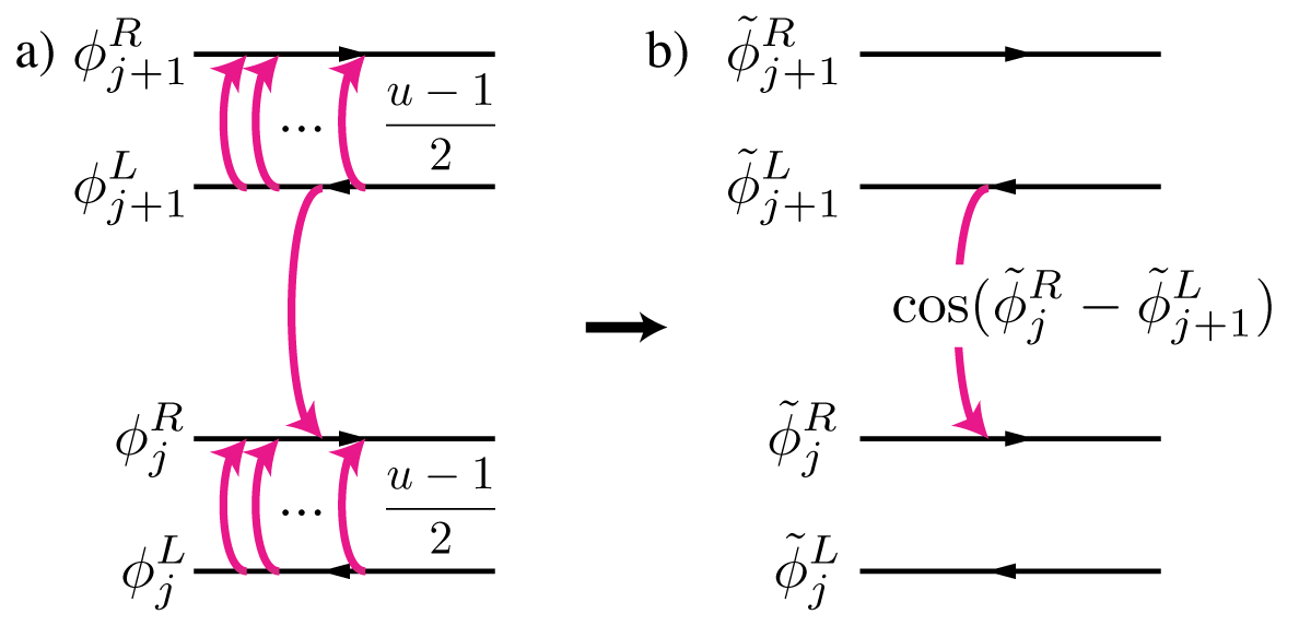
Figure 4: (a) The coupling that stabilises a $1/u$ Laughlin phase. (b) By locally rotating the Hilbert space on each wire in terms of new $\tilde{\phi}^{R/L}$ fields, the coupling from subplot (a) is re-expressed as a simple locking term between two fractionalised fields, see Eq. (33).

We start by introducing a change of basis on each wire, from our bare $\theta$ and $\varphi$ fields to a new set of fractionalised bosonic fields. This transformation is defined by a parameter $u\in\mathbb{N}$.

$$\tilde{\phi}^{R}_{j}(x) =\varphi_{j}(x)+u\theta_{j}(x),$$ (26)

$$\tilde{\phi}^{L}_{j}(x) =\varphi_{j}(x)-u\theta_{j}(x).$$ (27)

These new fields satisfy similar commutation relations to the bare fields, Eq. 12, although they are rescaled by a factor of $u$,

$$[\partial_{x}\tilde{\phi}^{p}_{j}(x),\tilde{\phi}^{q}_{k}(x^{\prime})]=\mp 2\pi iu\delta_{jk}\delta_{pq}\delta(x-x^{\prime}).$$ (28)

As we shall see in Section IV, these fields correspond to a pair of $1/u$-fractionalised chiral left and right movers.

Now all that remains is to construct an interaction that couples these fractionalised right and left movers between adjacent wires, which will ensure that the system as a whole is in a $1/u$ fractionalised phase. We consider a coupling between the wires at $j$ and $j+1$ given by the parameters

$$m_{j}=m_{j+1} =u,$$ (29)

$$n_{j} =+1,$$ (30)

$$n_{j+1} =-1.$$ (31)

A diagram of this coupling is shown in Fig. 4a. In terms of bosonic fields, this leads to a term of the form

$$\mathcal{O}(x)=\cos\left(\varphi_{j}+u\theta_{j}-\varphi_{j+1}+u\theta_{j+1}\right).$$ (32)

Comparing to Eqs. 26 and 27, we see that this coupling can be written as

$$\mathcal{O}(x)=\cos\left(\tilde{\phi}^{R}_{j}-\tilde{\phi}^{L}_{j+1}\right),$$ (33)

where we have coupled a fractionalised right mover from one wire onto the left mover on the wire above. Next, we transform to a new set of sum and difference fields,

$$\tilde{\varphi}_{j+\frac{1}{2}} =\frac{1}{2}\left(\tilde{\phi}_{j}^{R}(x)+\tilde{\phi}_{j+1}^{L}(x)\right),$$ (34)

$$\tilde{\theta}_{j+\frac{1}{2}} =\frac{1}{2}\left(\tilde{\phi}_{j}^{R}(x)-\tilde{\phi}_{j+1}^{L}(x)\right).$$ (35)

These sum and difference fields exist at the boundary between the $j$^th and $(j+1)$^th wires, which we will define as the $j+\frac{1}{2}$ quasiwire. In what follows, bare fermion $\theta$ and $\phi$ fields will be defined on the original wires, whereas the fractionalised $\tilde{\theta}$ and $\tilde{\phi}$ fields exist on these quasiwires.

We find that these have almost identical commutation relations to those satisfied by $\theta$ and $\varphi$, see Eqs. 20 and 21, aside from an additional factor of $u$,

$$[\partial_{x}\tilde{\theta}_{j+\frac{1}{2}}(x),\tilde{\varphi}_{k+\frac{1}{2}}(x^{\prime})] =\pi iu\delta_{jk}\delta(x-x^{\prime}),$$ (36)

$$[\partial_{x}\tilde{\theta}_{j+\frac{1}{2}}(x),\tilde{\theta}_{k+\frac{1}{2}}(x^{\prime})] =0,$$ (37)

$$[\partial_{x}\tilde{\varphi}_{j+\frac{1}{2}}(x),\tilde{\varphi}_{k+\frac{1}{2}}(x^{\prime})] =0.$$ (38)

Thus, the coupling becomes

$$\mathcal{O}(x)=\cos\left(2\tilde{\theta}_{j+\frac{1}{2}}\right).$$ (39)

This operator satisfies two properties that are necessary for the system to admit an exact solution: $\tilde{\theta}_{j+\frac{1}{2}}$ must commute between wires, and $\tilde{\theta}_{j+\frac{1}{2}}(x)$ must commute with $\tilde{\theta}_{j+\frac{1}{2}}(x^{\prime})$ when $x\neq x^{\prime}$. This ensures that all couplings across the $x$ and $y$ directions commute with one another, and thus can be independently satisfied in the ground state.

III.2 Gluing Fractions Together

Now, let us consider an interface between two sets of coupled wires, where we wish to enforce different fractionalisations ($u_{1}$ and $u_{2}$) in each wire, as shown in Fig. 5. Thus, we wish to couple a $u_{1}$-fractionalised mode, $\tilde{\phi}^{R}_{1}$, from the lower wire with a $u_{2}$-fractionalised mode, $\tilde{\phi}^{L}_{2}$, from the upper wire. This coupling must take an analogous form to Eq. 33, which preserves the exact solubility of the system. With that in mind, let us propose a trial coupling

$$\mathcal{O}(x)=\cos\left(b\tilde{\phi}^{R}_{1}-a\tilde{\phi}^{L}_{2}\right),$$ (40)

where $a$ and $b$ are a pair of parameters that we must choose. Note that we require $a,b\in\mathbb{Z}$ for it to be possible to express this coupling in terms of bare fermions.

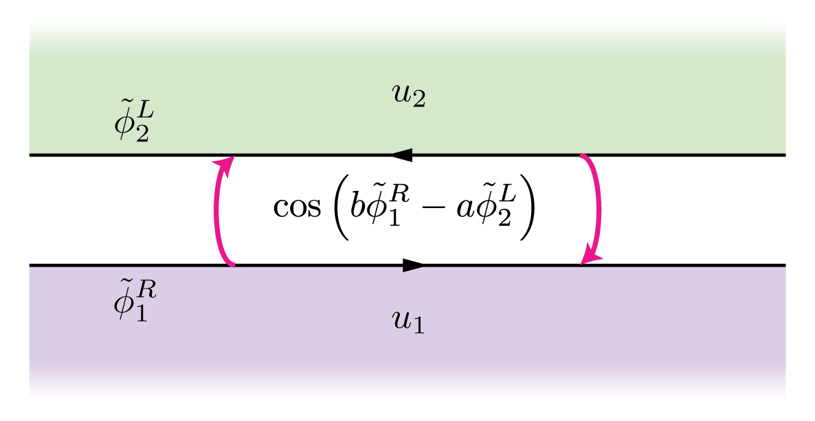
Figure 5: Two regions of coupled wires where the lower (purple) region forms a $1/u_{1}$ fractionalised Laughlin phase and the upper (green) region forms a $1/u_{2}$ phase. A coupling is introduced between the two respective edge modes that pairs $b$ $u_{1}$-quasiparticles with $a$ $u_{2}$-quasiparticles. By choosing appropriate values of $a$ and $b$ such that $u_{1}/u_{2}=a^{2}/b^{2}$, see Eq. (44), we can ensure the boundary remains gapped.

This coupling determines a pair of operators that play the same role as the $\tilde{\theta}$ and $\tilde{\varphi}$ operators presented in Eqs. 34 and 35,

$$\tilde{\theta}_{1.5}=\frac{1}{2}(b\tilde{\phi}^{R}_{1}-a\tilde{\phi}^{L}_{2}),$$ (41)

$$\tilde{\varphi}_{1.5}=\frac{1}{2}(b\tilde{\phi}^{R}_{1}+a\tilde{\phi}^{L}_{2}).$$ (42)

These should obey an analogous set of commutation relations as Eqs. 36, 37 and 38. In particular, for the coupling to preserve exact solubility, we require that $\tilde{\theta}_{1.5}$ commute with itself at different positions in space. Calculating this explicitly for $\tilde{\theta}$, we find that

$$[\partial_{x}\tilde{\theta}_{1.5}(x),\tilde{\theta}_{1.5}(x^{\prime})]=\frac{\pi i}{4}(u_{1}b^{2}-u_{2}a^{2})\delta(x-x^{\prime}).$$ (43)

Thus, we require

$$\frac{u_{1}}{u_{2}}=\left(\frac{a}{b}\right)^{2}$$ (44)

for $\tilde{\theta}_{1.5}$ to describe a conserved quantity. Since all variables here must be $\in\mathbb{Z}$. Thus, it is only possible to introduce such a coupling between a pair of fractionalised phases if the ratio between fractions is a square of a rational number. This is consistent with the so-called null-vector criterion proposed by Haldane [9], which is also discussed in detail in [164, 165]. Following this condition, let us write the fractionalisation coefficients $u_{1}$ and $u_{2}$ in terms of a common factor $u$, and our pair of integers $a$ and $b$, according to

$$u_{1} =ua^{2},$$ (45)

$$u_{2} =ub^{2},$$ (46)

We may now write the full commutation relations of the quasiparticle sum and difference operators, analogous to Eqs. 36, 37 and 38,

$$[\partial_{x}\tilde{\theta}_{1.5}(x),\tilde{\varphi}_{1.5}(x^{\prime})] =\pi iua^{2}b^{2}\delta(x-x^{\prime}),$$ (47)

$$[\partial_{x}\tilde{\theta}_{1.5}(x),\tilde{\theta}_{1.5}(x^{\prime})] =[\partial_{x}\tilde{\varphi}_{1.5}(x),\tilde{\varphi}_{1.5}(x^{\prime})]=0,$$ (48)

and the coupling between the two regions can be written in a familiar form

$$\mathcal{O}(x)=\cos\left(2\tilde{\theta}_{1.5}(x)\right).$$ (49)

III.2.1 Charge Conservation

Remarkably, we have seen that it is possible to introduce a coupling between two fractionalised phases with different fractionalisation, such that the boundary between the phases is gapped. However, such a coupling comes with a price, which is that we have violated charge conservation. To see how, let us convert our coupling back into bare fermion sum and difference fields using the identities

$$\tilde{\phi}_{1}^{R} =\varphi_{1}+ua^{2}\theta_{1},$$ (50)

$$\tilde{\phi}_{2}^{L} =\varphi_{2}-ub^{2}\theta_{2},$$ (51)

such that the coupling becomes

$$\mathcal{O}(x)=\cos\left(b\varphi_{1}-a\varphi_{2}+ua^{2}b\theta_{1}+uab^{2}\theta_{2}\right).$$ (52)

Thus, following the discussion in Section II.1, we see that such a term involves a net addition (or subtraction in the case of the hermitian conjugate) of $(a-b)$ bare fermions to the system. Taken alone, we see that this coupling does not respect charge conservation [164, 165]. However, as is shown in Appendix B, charge conservation may be restored by including an additional non-fractionalised wire which plays the role of a substrate. This exchanges charge with our system, but changes none of the properties of the fractionalised phase, and so we neglect to write explicitly it in what follows.

III.2.2 Momentum Conservation

We may additionally want to check that this coupling satisfies momentum conservation. Comparing with Eq. 11, we see that the condition imposed is

$$B(by_{1}-ay_{2})+k_{F}uab(a+b)=0.$$ (53)

Since we are free to choose the values of $y_{j}$, this condition is always satisfiable. Furthermore, this relation provides a correspondence between the relative fractionalisation of each wires and their positions in real space. Thus, in order to produce a composite phase where different wires have different fractionalisation, we necessarily must place wires at non-uniform separation from one another.

IV A General Construction for Non-Uniform Fractionalisation

We now have all the ingredients necessary to construct a generic composite fractionalised system. That is, given a set of wires, we have shown that it is possible to build couplings that can put each wire in a $1/{u_{j}}$ fractionalised phase . Additionally, we have seen that, provided all fractions take the form $u_{j}=ua_{j}^{2}$, with a common $u$ and all $a_{j}$ coprime, it is possible to introduce a coupling between each wire such that the system forms an overall gapped phase. This construction involves the series of transformations given above, which we compile in Appendix A for ease of use.

We now examine the properties of such a composite construction. In Section IV.1 we determine the degeneracy of the ground state, showing that by mixing fractionalised phases a composite system is able to realise phase with a ground state degeneracy distinct from any of the constituent phases. In Section IV.2 we review the definition of charge carried by every quasiparticle in the uniform Laughlin phase, following [102]. Next, extending to the disordered context, a notion of overall charge cannot be defined (see Section III.2.1), however we define and calculate a quantity analogous to charge, which is conserved. Finally, in Section IV.3 we discuss the braiding of excitations in such a composite fractional material. We explicitly calculate their exchange statistics and show how the system divides into composite fractionalised anyons which are free to move throughout the system, and lineons which can only propagate in the $x$-direction.

Let us start by establishing the most generic configuration, in which we have an array of $N$ wires at positions $y_{j}$. We wish to place each wire in a $1/{u{a_{j}^{2}}}$-fractionalised phase. Thus, we write the degrees of freedom of each wire in terms of left and right-moving fractionalised bosonic fields, $\tilde{\phi}_{j}^{L/R}$, whose commutator includes a factor of $ua_{j}^{2}$, following Eq. 28.

We place a coupling between each pair of adjacent wires that takes the form $\cos(2\tilde{\theta}_{j+\frac{1}{2}})$, with

$$\tilde{\theta}_{j+\frac{1}{2}} =\frac{1}{2}\left(a_{j+1}\tilde{\phi}_{j}^{R}-a_{j}\tilde{\phi}_{j+1}^{L}\right),$$ (54)

$$\tilde{\varphi}_{j+\frac{1}{2}} =\frac{1}{2}\left(a_{j+1}\tilde{\phi}_{j}^{R}+a_{j}\tilde{\phi}_{j+1}^{L}\right).$$ (55)

Thus, the overall Hamiltonian is

$$H=H_{\textup{Kin}}+\int\frac{dx}{2\pi}\sum_{j}\cos\left(2\tilde{\theta}_{j+\frac{1}{2}}(x)\right),$$ (56)

where $H_{\textup{Kin}}$ is a quadratic function in $\{\partial_{x}\tilde{\theta}_{j+\frac{1}{2}}\}$ and $\{\partial_{x}\tilde{\varphi}_{j+\frac{1}{2}}\}$. Let us parametrise $H_{\textup{Kin}}$ in terms of a $2N\times 2N$ matrix $M$ as

$$H_{Kin}=\int\frac{dx}{2\pi}\begin{pmatrix}\partial_{x}\tilde{\bm{\varphi}}\\ \partial_{x}\tilde{\bm{\theta}}\end{pmatrix}^{T}\begin{pmatrix}M_{\varphi\varphi}&M_{\theta\varphi}\\ M_{\varphi\theta}&M_{\theta\theta}\end{pmatrix}\begin{pmatrix}\partial_{x}\tilde{\bm{\varphi}}\\ \partial_{x}\tilde{\bm{\theta}}\end{pmatrix},$$ (57)

where $\tilde{\bm{\varphi}}$ represents the column vector $\begin{pmatrix}\tilde{\varphi}_{0.5}&...&\tilde{\varphi}_{N-\frac{1}{2}}\end{pmatrix}^{T}$, with a similar expression for $\tilde{\bm{\theta}}$.

Since the coupling is expressed exclusively in terms of the difference field $\tilde{\theta}$, the only condition for the model to remain solvable is that terms involving $\tilde{\varphi}$ (which does not commute with $\tilde{\theta}$) are weak. In the usual bosonisation limit $M_{\varphi\varphi}=M_{\theta\varphi}=M_{\varphi\theta}=0$, so all terms in $H$ commute precisely, and thus we may treat $\tilde{\theta}$ as a classical variable, replacing it with its expectation value. Thus, the system sits in a gapped ground state defined by the lowest energy configuration of $\{\tilde{\theta}_{j+\frac{1}{2}}\}$.

Provided that no terms in $H_{\textup{Kin}}$ involving $\tilde{\varphi}$ are strong enough to close the gap to the $\tilde{\theta}$-ordered ground state, we can effectively treat the system as fluctuating close to this exact, effectively classical, ground state. In what follows, we shall assume that we are working in this limit, the conventional limit where such bosonisation constructions are valid [102, 103, 104].

At this point, the Hamiltonian has been reduced to an interplay between two sets of terms: coupling terms, which are minimised when all fields are fixed to a multiple of $\pi$, and kinetic terms quadratic in $\partial_{x}\tilde{\theta}$, which penalise spatially changing $\tilde{\theta}$ and vanish when it is constant. Thus, it is straightforward to write down the ground state which satisfies both terms: All fields are spatially uniform and pinned to a multiple of $\pi$,

$$\tilde{\theta}_{j+\frac{1}{2}}(x)=\tilde{\theta}_{j+\frac{1}{2}}\in\pi\mathbb{Z}.$$ (58)

IV.1 Ground State Degeneracy

Clearly, our system has some degree of ground state degeneracy. The only requirement to minimise the energy is that every $\tilde{\theta}$ sits at an integer value, and each field has an infinite number of such values that it can take. Thus, one might naively expect that the ground state has infinite degeneracy. To avoid this contradiction, some configurations of $\tilde{\theta}$ must be equivalent. To see how, note that by bosonising we introduced a spurious degree of freedom. A fermionic field is unchanged under a trivial transformation $\psi\rightarrow e^{2i\pi}\psi$, so adding a multiple of $2\pi$ to the bare fermion bosonic fields also cannot correspond to a physical change in the system. Note that a similar calculation of the ground state degeneracy for a uniformly spaced set of wires, can be found in [170].

With this in mind, let us consider a system of $N$ coupled wires with periodic boundaries in both the $x$ and $y$ directions. That is, the $(N/2-1)^{\textup{th}}$ wire is coupled to the $(-N/2)^{\textup{th}}$ wire. We shall assume that the system is in a ground state, each pair of wires has a uniform value of $\braket{\theta_{j+\frac{1}{2}}(x)}$ pinned to a multiple of $\pi$.

Within this system, we focus (without loss of generality) on a set of three wires at positions $j=0,1,2$, each set to fractions $ua_{j}^{2}$, and introduce the following gauge transformation on the $1^{\textup{st}}$ wire,

$$\phi_{1}^{R} \rightarrow\phi_{1}^{R}+2\pi\alpha,$$ (59)

$$\phi_{1}^{L} \rightarrow\phi_{1}^{L}+2\pi\beta,$$ (60)

with parameters $\alpha,\beta\in\mathbb{Z}$. Under this transformation, our sum and difference fields Eqs. 18 and 19 change according to

$$\varphi_{1}\rightarrow\varphi_{1}+(\alpha+\beta)\pi,$$ (61)

$$\theta_{1}\rightarrow\theta_{1}+(\alpha-\beta)\pi.$$ (62)

Thus, let us define a new pair of variables $\gamma=\alpha+\beta$ and $\delta=\alpha-\beta$. Given that $\alpha$ and $\beta$ are free to take any integer value, we see that $\gamma$ and $\delta$ can also take any value provided they are both even or both odd. Following the transformation through to the couplings, we find that

$$2\tilde{\theta}_{1.5} \rightarrow 2\tilde{\theta}_{1.5}+\left(\gamma+ua_{1}^{2}\delta\right)a_{2}\pi,$$ (63)

$$2\tilde{\theta}_{0.5} \rightarrow 2\tilde{\theta}_{0.5}+\left(-\gamma+ua_{1}^{2}\delta\right)a_{0}\pi.$$ (64)

Let us consider two cases. First we shall look at the case of a uniform Laughlin phase ($a_{j}=1,\forall j$) and verify the known result that a phase with $1/u$ fractionalised quasiparticles should have a $u$-fold degenerate ground state. Then we shall extend the analysis to the general case ($a_{j}\neq 1$), finding the degeneracy of a general composite system.

The Uniform Case: Setting all $a_{j}=1$, we ensure all wires have the same fractionalisation. Let us consider the effect of two gauge transformations, where any other gauge transformation can be produced by successively applying these two. Thus, a quantity that is invariant under these two is gauge invariant in general.

First we look at the transformation parametrised by $\gamma=2,\delta=0$. The effect on our fields is

$$\tilde{\theta}_{1.5} \rightarrow\tilde{\theta}_{1.5}+\pi,$$ (65)

$$\tilde{\theta}_{0.5} \rightarrow\tilde{\theta}_{0.5}-\pi.$$ (66)

Successively applying such a transformation on different wires allows one to make any change to the $\tilde{\theta}$ values that preserves $\sum_{j}\tilde{\theta}_{j+\frac{1}{2}}$.

Next, we consider a transformation parametrised by $\gamma=1,\delta=1$. The effect on our fields is

$$\tilde{\theta}_{1.5} \rightarrow\tilde{\theta}_{1.5}+\frac{u+1}{2}\pi,$$ (67)

$$\tilde{\theta}_{0.5} \rightarrow\tilde{\theta}_{0.5}+\frac{u-1}{2}\pi.$$ (68)

Thus, we see that under such a transformation, the value of $\sum_{n}\tilde{\theta}_{j+\frac{1}{2}}$ changes by

$$\sum_{n}\tilde{\theta}_{j+\frac{1}{2}}\rightarrow\sum_{n}\tilde{\theta}_{j+\frac{1}{2}}+u\pi.$$ (69)

Thus, we propose that the only gauge invariant quantity one can derive from the values of $\tilde{\theta}$ is

$$A_{GS}=\frac{1}{\pi}\sum_{n}\tilde{\theta}_{j+\frac{1}{2}}\mod u.$$ (70)

Since $A_{GS}$ can take $u$ possible integer values, we find that the number of degenerate ground states is

$$N_{GS}=u,$$ (71)

which is the expected ground state degeneracy for a $1/u$ Laughlin phase.

The Non-uniform Case— We now revisit the same argument, while allowing for $a_{j}\neq 1$. Additionally, let us also require (without loss of generality) that all adjacent $a_{j}$ values are coprime, since any common factors may be absorbed into $u$. First, considering the transformation $\gamma=2,\delta=0$, we find an overall change to our fields of

$$\frac{\tilde{\theta}_{1.5}}{a_{1}a_{2}} \rightarrow\frac{\tilde{\theta}_{1.5}}{a_{1}a_{2}}+\frac{\pi}{a_{1}},$$ (72)

$$\frac{\tilde{\theta}_{0.5}}{a_{0}a_{1}} \rightarrow\frac{\tilde{\theta}_{0.5}}{a_{0}a_{1}}-\frac{\pi}{a_{1}}.$$ (73)

Thus, in this case, let us propose the following candidate for our overall conserved quantity:

$$A_{GS}=\frac{1}{\pi}\sum_{j}\frac{\tilde{\theta}_{j+\frac{1}{2}}}{a_{j}a_{j+1}}.$$ (74)

Next, we once again consider the $\gamma=1,\delta=1$ gauge transformation, which produces a change in our fields of

$$\frac{\tilde{\theta}_{1.5}}{a_{1}a_{2}} \rightarrow\frac{\tilde{\theta}_{1.5}}{a_{1}a_{2}}+\left(ua_{1}+\frac{1}{a_{1}}\right)\frac{\pi}{2},$$ (75)

$$\frac{\tilde{\theta}_{0.5}}{a_{0}a_{1}} \rightarrow\frac{\tilde{\theta}_{0.5}}{a_{0}a_{1}}+\left(ua_{1}-\frac{1}{a_{1}}\right)\frac{\pi}{2},$$ (76)

under which the total value of $A_{GS}$ changes by

$$A_{GS}\rightarrow A_{GS}+ua_{1}.$$ (77)

Similarly, choosing any other wire, we are free to perform such a gauge transformation, adding $\pm ua_{j}$ to the value of $A_{GS}$, for any $a_{j}$ present in the system. This means that, starting at an arbitrary value of $A_{GS}$, we may freely gauge transform to any other value that can be written in the form

$$A_{GS}\rightarrow A_{GS}+u\sum_{j}w_{j}a_{j},$$ (78)

where the sum is over all wires, with arbitrary $w_{j}\in\mathbb{Z}$. Since all $a_{j}$ are coprime, we invoke Bezout’s identity [171], which states that the sum on the right can be made to equal to any multiple of $u$ by choosing appropriate values of $\{a_{j}\}$. Thus, any pair of configurations for which $A_{GS}$ differs by a multiple of $u$ must be gauge equivalent.

All that remains is to determine how many gauge-inequivalent values of $A_{GS}$ exist. Since each $\tilde{\theta}$ field can take any value that is a multiple of $\pi$, the overall value of $A_{GS}$ can always be expressed in the form

$$A_{GS} =\frac{1}{\pi}\sum_{j}\frac{\tilde{\theta}_{j+\frac{1}{2}}}{a_{j}a_{j+1}},$$ (79)

$$=\frac{1}{\pi}\sum_{j}\left(\frac{b_{j}}{a_{j}}+\frac{b_{j+1}}{a_{j+1}}\right),$$ (80)

where $b_{j},b_{j+1}\in\mathbb{Z}$ must be chosen to satisfy $b_{j}a_{j+1}+b_{j+1}a_{j}=\tilde{\theta}_{j+\frac{1}{2}}$. Since the $a$ are coprime, we state two consequences of Bezout’s identity [171]. Firstly, $b_{j}$ and $b_{j+1}$ can be chosen for any $\tilde{\theta}_{j+\frac{1}{2}}$. Secondly, $\tilde{\theta}_{j+\frac{1}{2}}$ can be chosen such that $b_{j}$ takes any value mod $a_{j}$, and $b_{j+1}$ takes any value mod $a_{j+1}$ .

Consequently, $A_{GS}$ for the whole system can take any value that may be written as

$$A_{GS}=w+\sum_{j}\frac{b_{j}}{a_{j}},$$ (81)

with $w$ and all $b_{j}$ arbitrarily chosen integers. Thus, there are a total of $\prod_{j}a_{j}$ unique values of $A_{GS}$ between 0 and 1, and thus on any integer-length interval $[x,x+1)$. Note that this product is over all unique values of $a_{j}$ in the system.

Finally, since two configurations are gauge-equivalent only when they differ by a multiple of $u$, the number of degenerate ground states of the composite system is

$$N_{GS}=u\prod_{j}a_{j},$$ (82)

where the product is again over all unique values of $a_{j}$ present in the system.

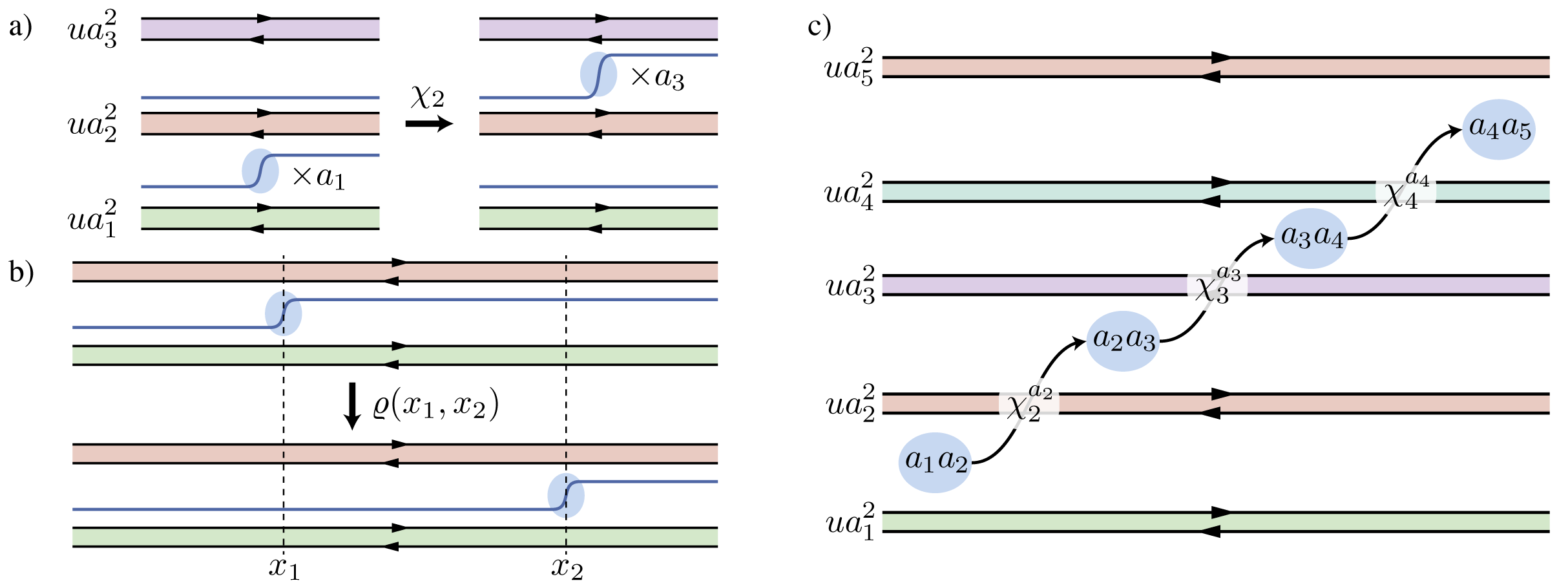
Figure 6: Transport of anyons through a system of fractionalised wires. Each wire may be differently fractionalised with $ua_{j}$, indicated by colour, as well as being unevenly displaced from one another. (a) The $\chi$ operator, Eq. 90, is responsible for transport in the $y$-direction. On a set of three coupled wires, the $\chi_{2}(x)$ operator destroys a composite of $a_{1}$ quasiparticles on the $\tilde{\theta}_{1.5}$ quasiwire, and creates a composite of $a_{3}$ quasiparticles from the $\tilde{\theta}_{2.5}$ quasiwire. (b) The $\rho$ operator, Eq. (95), is responsible for transport in the $x$-direction, where the operator $\rho(x_{1},x_{2})$ destroys a single kink at position $x_{1}$ and creates one at $x_{2}$ on the same wire. (c) On a given $\tilde{\theta}_{j+\frac{1}{2}}$ quasiwire, a composite excitation with $a_{j}a_{j+1}$ multiplicity can travel freely to the quasiwire above and below by applying the $\chi_{j}$ operator $a_{j}$ times. Furthermore, the nature of the $\chi$ operator is such that it ensures the new quasiparticle is always created with the correct multiplicity to allow it to travel onto the wire beyond.

IV.2 Quasiparticle Charge

We have seen that the ground state degeneracy of the system of coupled wires has a non-trivial dependence on the fractionalisation of all constituent wires in the system. Since the ground state degeneracy is related to the nature of the quasiparticle excitations, let us now explicitly derive the properties of these excitations.

Quasiparticles in the bosonised system correspond to a kink in $\tilde{\theta}_{j+\frac{1}{2}}$, where the value jumps by $\pm\pi$. As a warm-up, let us start by determining the bare charge carried by quasiparticles in the well-studied uniform case (all $a_{j}=1$), and then move on to the more involved non-uniform case.

The Uniform Case: Following Eq. 25, we may write down the expression for the total bare fermion charge contained on the $j^{\textup{th}}$ wire within a region $x_{I}\rightarrow x_{F}$ as

$$Q_{j}(x_{I},x_{F}) =\int_{x_{I}}^{x_{F}}\frac{dx}{2\pi}\rho_{j}(x),$$ (83)

$$=\left[\frac{\theta_{j}(x)}{\pi}\right]_{x_{I}}^{x_{F}}.$$ (84)

Using Eqs. 27, 26, 34 and 35 we may now re-express the bare density in terms of our fractionalised density variables $\tilde{\varphi}$ and $\tilde{\theta}$,

$$\frac{\theta_{j}(x)}{\pi}=\frac{1}{2u\pi}\left(\tilde{\varphi}_{j+\frac{1}{2}}-\tilde{\varphi}_{j-\frac{1}{2}}+\tilde{\theta}_{j+\frac{1}{2}}+\tilde{\theta}_{j-\frac{1}{2}}\right).$$ (85)

Now, taking a sum over a number of wires from $j=1$ to $j=N$, we find that terms with $\tilde{\varphi}$ cancel out in the bulk of the region, leaving

$$\begin{aligned} \sum_{j=1}^{N}\frac{\theta_{j}(x)}{\pi}&=\frac{1}{u}\sum_{j=1}^{N-1}\frac{\tilde{\theta}_{j+\frac{1}{2}}}{\pi}+\left(\textup{boundary terms}\right),\end{aligned}$$ (86)

where the boundary terms exist only on the $1^{\textup{st}}$ and $N^{\textup{th}}$ wires, so we neglect them. Thus, we see from Eq. (83) that a kink where $\tilde{\theta}_{j+\frac{1}{2}}$ changes by $\pi$ within the bulk of the region must correspond to adding a fractional charge of $1/u$.

The Non-uniform Case: We may once again re-express the bare fermion density in terms of fractionalised fields, although we now must use Eqs. 54 and 55, to get

$$\frac{\theta_{j}}{\pi}=\frac{1}{2ua_{j}\pi}\left(\frac{\tilde{\varphi}_{j+\frac{1}{2}}}{a_{j}a_{j+1}}-\frac{\tilde{\varphi}_{j-\frac{1}{2}}}{a_{j}a_{j-1}}+\frac{\tilde{\theta}_{j+\frac{1}{2}}}{a_{j}a_{j+1}}+\frac{\tilde{\theta}_{j-\frac{1}{2}}}{a_{j}a_{j-1}}\right).$$ (87)

By considering the denominators in this expression, we see that there are no neat cancellations in $\sum_{j}{\theta_{j}}$, which now retains dependence both on the $\tilde{\varphi}$ and $\tilde{\theta}$ fields in the bulk. This is unsurprising, since we have already established that bare fermionic charge is not conserved in the composite system, see Section III.2.1, unless a substrate is included, see Appendix B. Thus, we should not be surprised to see that overall charge does not have a well-defined expectation value. Rather, let us consider the quantity

$$\sum_{j=1}^{N}\frac{a_{j}\theta_{j}}{\pi} =\frac{1}{u\pi}\sum_{j=1}^{N-1}\frac{\tilde{\theta}_{j+\frac{1}{2}}}{a_{j}a_{j+1}}+\left(\textup{boundary terms}\right).$$ (88)

Since this is expressed only in terms of $\tilde{\theta}$, it is conserved and has a well-defined expectation value close to the ground state.

IV.3 Composite Statistics

In this section, we calculate anyonic braiding statistics. This calculation takes three parts. In the first we establish the operators necessary to transport anyons throughout the system. Next, we see how the properties of these transport operators lead to the emergence of two types of excitation: a set of composite anyons that are free to travel throughout the system along both axes, and a set of lineons which are confined to move only in the $x$-direction [173, 174]. Finally, we braid both sets of anyons and calculate relative statistics.

IV.3.1 Moving Anyons

Between Quasiwires—Let us first consider the backscattering of a single fermion from $R$ to $L$ on a single wire, represented by the following operator,

$$\begin{aligned} \chi_{j}(x)=&{\psi^{L}_{j}}^{\dagger}(x){\psi^{R}_{j}}_{j}(x)\\ &\rightarrow e^{-i[\phi^{R}_{j}(x)-\phi^{L}_{j}(x)]}.\end{aligned}$$ (89)

Re-expressed in terms of fractionalised fields, this takes the form

$$\chi_{j}(x)=\exp\left(\frac{-i}{ua_{j}^{2}}[\tilde{\phi}^{R}_{j}(x)-\tilde{\phi}^{L}_{j}(x)]\right).$$ (90)

We now compute the effect of $\chi_{j}(x)$ on the $\partial_{x}\tilde{\theta}(x^{\prime})$ fields,

$$[\partial_{x}\tilde{\theta}_{j+\frac{1}{2}}(x),\chi_{j}(x^{\prime})] =\pi a_{j+1}\delta(x-x^{\prime})\chi_{j}(x^{\prime}),$$ (91)

$$[\partial_{x}\tilde{\theta}_{j-\frac{1}{2}}(x),\chi_{j}(x^{\prime})] =-\pi a_{j-1}\delta(x-x^{\prime})\chi_{j}(x^{\prime}),$$ (92)

which we use to derive the following identities,

$$\chi_{j}^{-1}\partial_{x}\tilde{\theta}_{j+\frac{1}{2}}\chi_{j}=\partial_{x}\tilde{\theta}_{j+\frac{1}{2}}+\pi a_{j+1}\delta(x-x^{\prime}),$$ (93)

$$\chi_{j}^{-1}\partial_{x}\tilde{\theta}_{j-\frac{1}{2}}\chi_{j}=\partial_{x}\tilde{\theta}_{j-\frac{1}{2}}-\pi a_{j-1}\delta(x-x^{\prime}),$$ (94)

where $\chi$ acts at $x^{\prime}$ and $\partial\tilde{\theta}$ acts at $x$. Thus, we see see that the operator removes $a_{j-1}$ quasiparticles on the $\tilde{\theta}_{j-\frac{1}{2}}$ quasiwire and creates $a_{j+1}$ quasiparticles on the $\tilde{\theta}_{j+\frac{1}{2}}$ quasiwire. A diagram is shown in Fig. 6a. Thus, we see that in the $y$-direction, quasiparticles can only be moved in groups of $a_{j}$.

Along Quasiwires—The operator that transfers a quasiparticle from $x_{1}$ to $x_{2}$ along the $j+1/2$ quasiwire is

$$\varrho_{j+\frac{1}{2}}(x_{1},x_{2}) =\exp\left(i\frac{\tilde{\varphi}_{j+\frac{1}{2}}(x_{1})-\tilde{\varphi}_{j+\frac{1}{2}}(x_{2})}{{ua_{j}^{2}a_{j+1}^{2}}}\right),$$ (95)

$$=\exp\left(i\frac{\int_{x_{2}}^{x_{1}}\mathrm{d}x\,\partial_{x}\tilde{\varphi}_{j+1/2}(x)}{ua_{j}^{2}a_{j+1}^{2}}\right),$$ (96)

which is a local operator since $\partial_{x}\tilde{\varphi}$ can always be written in terms of the bare fermion densities, see Eq. 15. This operator allows us to transport a single $\pm\pi$ kink along a wire to any arbitrary position.

IV.3.2 Lineons and Composite Anyons

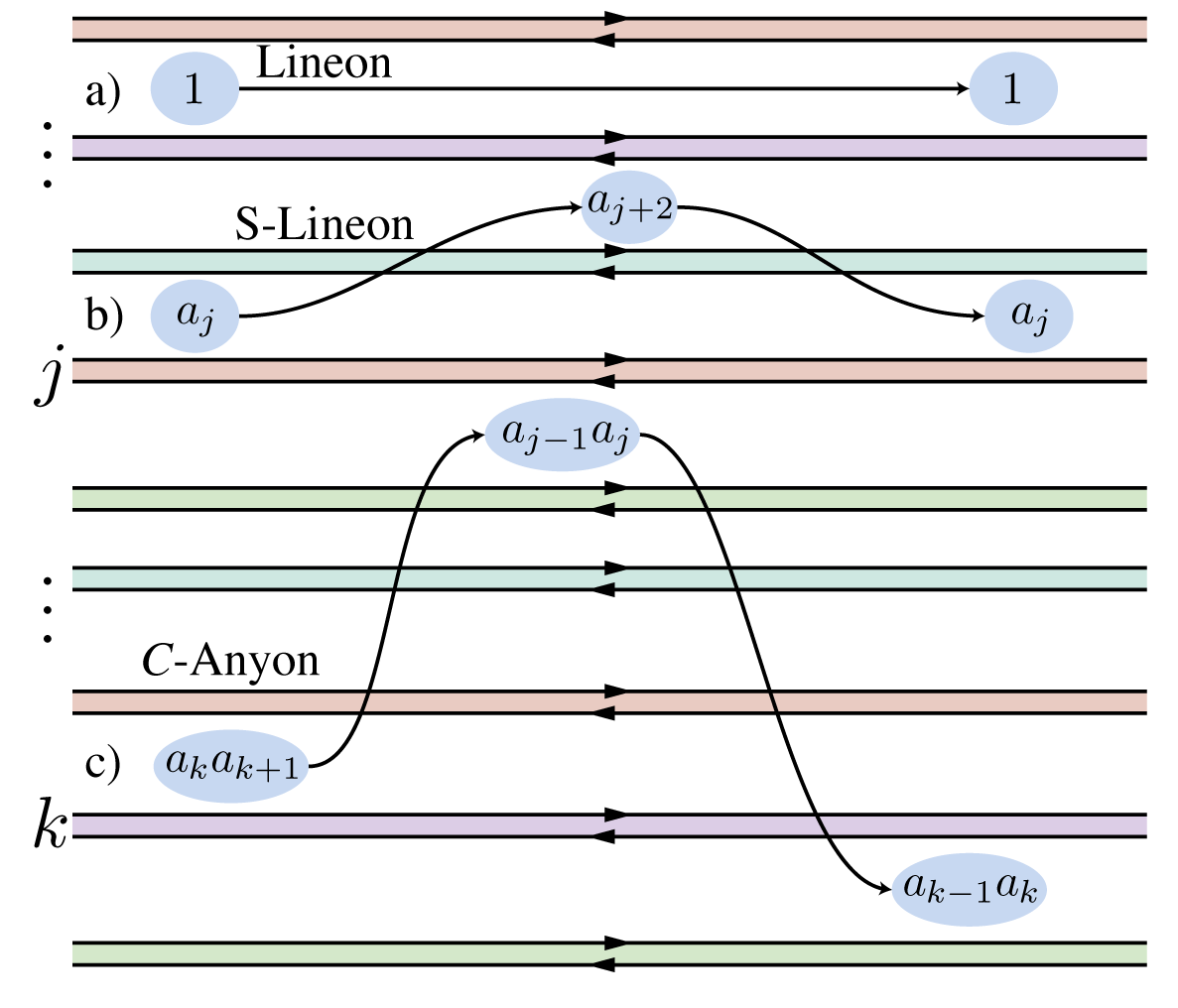
Figure 7: Three types of fractionalised excitations in a system of unevenly spaced wires, where the $j$^th wire is in a $1/ua_{j}^{2}$ phase. (a) A single kink between the $j$ and $j+1$ wire corresponds to an excitation carrying ${1}/{ua_{j}^{2}a_{j+1}^{2}}$ statistics, and is constrained to only move in the $x$ direction. (b) A composite of $a_{j}$ kinks between the $j$ and $j+1$ wire is only able to travel up to the next wire and back. (c) Finally, a $C$-anyon, a composite of $a_{k}a_{k+1}$ kinks has complete freedom to travel throughout the system. Note that (a) and (b) are fractons, constrained to move in the $x$-direction, whereas (c) is not constrained.

Following the form of the above quasiparticle transport operators Eqs. 90 and 95, we see that the $x$ and $y$-directions in our model effectively ‘see’ a different type of quasiparticle. In the $x$-direction, each quasiparticle is free to move independently along the wire. However, in the $y$-direction quasiparticles can only be transported together in groups of $a_{j}$, where each interface between wires with a different value of $a_{j}$ thus transfers a different number of quasiparticles, as shown in Fig. 6. Thus, it is natural to ask if there is a minimal combined quasiparticle that is free to travel throughout the system in both directions.

To answer this, we consider a set of $\eta$ quasiparticles at the same position on a quasiwire at $\tilde{\theta}_{j+\frac{1}{2}}$. In order to be able to travel freely in the $y$-direction, we must at least be able to hop this set of quasiparticles both onto the quasiwire above and the one below. Thus, there are two $\chi$ operators to consider, following Eqs. 91 and 92. To move the bundle up to the next wire, we must apply a $\chi_{j+1}$ operator, which destroys $a_{j}$ kinks and creates $a_{j+2}$ kinks on the next quasiwire. Similarly, to move the bundle down, we must apply a $\chi_{j}^{\dagger}$ operator, which destroys $a_{j+1}$ kinks and creates $a_{j-1}$ on the quasiwire below. Thus, for this bundle of quasiparticles to be freely mobile, we must have started with a number $\eta$ of particles in the bundle that is both divisible by $a_{j}$ and $a_{j+1}$. Since all $a_{j}$ are coprime, the minimal acceptable bundle contains $a_{j}\times a_{j+1}$ quasiparticles.

Now, suppose we start with such a bundle of $a_{j}\times a_{j+1}$ quasiparticles on the $\tilde{\theta}_{j+\frac{1}{2}}$ quasiwire and wish to transport it to the quasiwire above. Since $\chi_{j+1}$ only moves $a_{j}$ individual quasiparticles, we will have to apply it $a_{j+1}$ times. Each time we destroy $a_{j}$ particles and create $a_{j+2}$ particles on the next wire. Thus, we finish having removed the full bundle, and created a bundle of $a_{j+1}\times a_{j+2}$ quasiparticles on the quasiwire above, at $\tilde{\theta}_{j+1,j+2}$. Remarkably, the transport operators conspire to ensure that the bundle created on the next wire has the right multiplicity to allow it to hop onto the wire above, and so on. A diagram of this process is shown in Fig. 6c.

Excitations in the system can thus be classified broadly into three types. One has a set of fractionalised quasiparticles corresponding to a single $\pm\pi$ kink on a given quasiwire. These are constrained to only move in the $x$-direction – constituting a set of fractonic excitations called lineons [173, 174]. Next, we may combine a group of $a_{j}$ such excitations to form a constrained compound particle, which can only hop over one adjacent wire, but no further. These have also constrained motion as lineons, but are spread among two wires, and hence we refer to them as spread-lineons, or s-lineons for short. Finally, combining $a_{j}\times a_{j+1}$ fractonic quasiparticles on the $\tilde{\theta}_{j+\frac{1}{2}}$ quasiwire produces a free composite quasiparticle that may travel unimpeded throughout the system. We shall label these as $C$-particles. These three cases are shown in Fig. 7.

IV.3.3 Braiding

Let us now calculate the braiding statistics of the anyons in our system. Only $C$-type composite particles can be transported freely around the system, whereas lineons can only participate by having a $C$-type quasiparticle moved around them. Note that, for the braiding statistics to pick up only a topological phase, one must perform braiding with all quasiparticles well-separated in space. Bringing kinks close to one another changes the energy of the system, causing the phase to precess. To avoid this, we assume that quasiparticles are always well-separated throughout the braiding operation.

To determine the braiding statistics, we must first examine the $\chi$ operators responsible for moving a kink between wires. Starting with Eq. 90, we rewrite the term in the exponential as

$$\tilde{\phi}^{R}_{j}(x)-\tilde{\phi}^{L}_{j}(x)=\frac{\tilde{\varphi}_{j+\frac{1}{2}}+\tilde{\theta}_{j+\frac{1}{2}}}{a_{j+1}}-\frac{\tilde{\varphi}_{j-\frac{1}{2}}-\tilde{\theta}_{j-\frac{1}{2}}}{a_{j-1}}.$$ (97)

Next, we consider the operation that moves a single $C$-particle throughout the system, shown in Fig. 6c, where we apply each $\chi_{j}$ operator $a_{j}$ times. Since $\chi$ on different wires commute, we may write the overall operator that transports a $C$-particle from the $(j-\frac{1}{2})$^th to the $(k+\frac{1}{2})$^th quasiwire as the following product of operators,

$$\prod_{i=j}^{k}\chi_{i}^{a_{i}}(x)=\exp\left(\frac{-i}{u}\sum_{i=j}^{k}\frac{\tilde{\phi}^{R}_{i}(x)-\tilde{\phi}^{L}_{i}(x)}{a_{i}}\right),$$ (98)

inserting Eq. 97, we find that all $\tilde{\varphi}$ operators cancel out aside from those at the endpoints,

$$\prod_{i=j}^{k}\chi_{i}^{a_{i}}(x)=\exp\left(-i\sum_{i=j}^{k-1}\frac{2\tilde{\theta}_{i,i+1}}{ua_{i}a_{i+1}}+\hat{\mathcal{O}}_{\textup{endpoints}}\right),$$ (99)

with

$$\hat{\mathcal{O}}_{\textup{endpoints}}=-i\left(\frac{\tilde{\phi}^{R}_{k}}{ua_{k}}-\frac{\tilde{\phi}^{L}_{j}}{ua_{j}}\right).$$ (100)

We have split the operator into two terms. $\hat{\mathcal{O}}_{\textup{endpoints}}$ is responsible for destroying $a_{j-1}a_{j}$ quasiparticles on the $j+\frac{1}{2}$ quasiwire and creating $a_{k}a_{k+1}$ quasiparticles on the $k,k+1$ quasiwire. We find an additional term in Eq. 99 which adds a phase that depends on the absolute value of $\tilde{\theta}$ along the path from $j$ to $k$. Since we are working on the assumption $\tilde{\theta}$ has well-defined expectation value, we see that the effect of this term is simply to apply a global phase of

$$\gamma=\sum_{i=j}^{k-1}\frac{2\braket{\tilde{\theta}_{i,i+1}(x)}}{ua_{i}a_{i+1}}$$ (101)

to the wavefunction of our system.

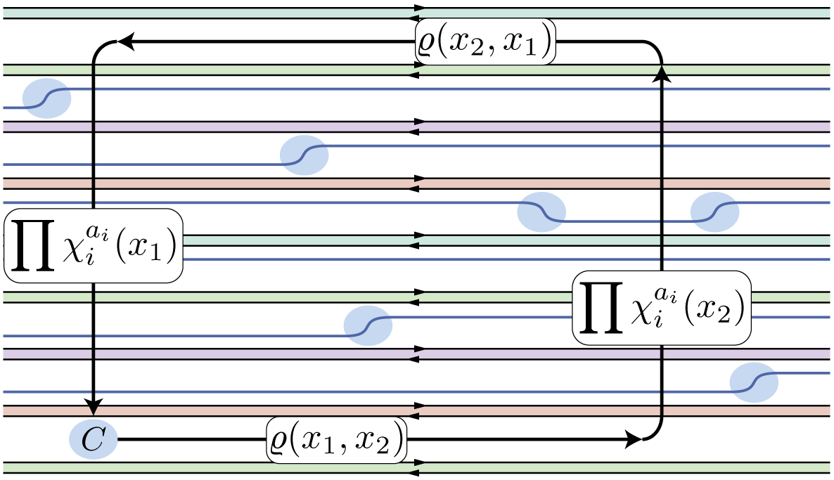
Figure 8: A single $C$-quasiparticle is transported around a loop, shown in black, with the corresponding operator for each section of the loop shown explicitly. Quasiparticles encircled by this loop lead to a difference in $\tilde{\theta}$ measured by the $C$-particle on the two sections where it moves in the $y$-direction. Thus, the overall phase accumulated on the path is a direct measure of the number of kinks contained inside the loop.

Thus, let us consider moving a single $C$-type quasiparticle around a loop in the system, as shown in Fig. 8. Such an operation involves four operators. In the $x$-direction, we require two $\varrho$ operators. We work under the assumption that there are no other quasiparticles obstructing the translation of our $C$ anyon along its path—so that the phase does not precess with any non-topological phases. Thus, transport in the $x$-direction has no effect on the phase accumulated around this loop.

However, as we have just seen, transporting a kink in the $y$ direction causes the system to accumulate a phase that depends on the value of $\tilde{\theta}$ along the path. Thus, the full loop picks up an overall phase of

$$\gamma_{\textup{loop}}=\sum_{i=j}^{k-1}\frac{2\braket{\tilde{\theta}_{i,i+1}(x_{2})}-2\braket{\tilde{\theta}_{i,i+1}(x_{1})}}{ua_{i}a_{i+1}}.$$ (102)

This term exactly counts the number of kinks inside the encircled region, since each single kink leads to a $\Delta\tilde{\theta}$ of $\pi$ between the left and right side of the loop.

We can read the mutual statistics of our anyons directly from Eq. 102. A single fractonic quasiparticle contributes a phase of $2\pi/ua_{j}a_{j+1}$ when encircled by a $C$-particle, whereas a $C$-type particle appears with multiplicity $a_{j}a_{j+1}$, and so contributes a total phase of $2\pi/u$. Thus, such C-anyons act like Laughlin quasiparticles fractionalised with the common divisor of all constituent fractions in the system. Finally, a pair of s-lineons may be braided around one another, across the only wire they are able to cross (which we choose to be the $j$^th wire for this example), incurring a phase of $2\pi/ua_{j}^{2}$—the fractionalisation of their shared wire.

V Discussion and Conclusions

In summary, we have provided an exactly solvable model for a non-crystalline topological order that displays qualitatively different phenomenology to its crystalline counterpart. To do so, we have extended the coupled-wire construction of the fractional Hall effect to non-crystalline systems, considering the properties of inhomogeneous arrays of coupled wires. Conservation of momentum requires an inhomogeneous system to also have inhomogeneous couplings, which ensure that different parts of the system have differently fractionalised excitations. Adjacent regions with different fractionalisation may then be coupled to one another in such a way that the system as a whole remains gapped and solvable. This is possible provided the ratio of each fractionalisation is a square of a rational number, which we enforce by setting each region’s fractionalisation to an integer $ua_{j}^{2}$. This has allowed us to propose a general and solvable construction for composite, and disordered, fractionalised systems.

The phenomenology of the resulting fractionalized phase is determined by the non-uniformity, and differs significantly from the uniform case. The ground state degeneracy depends non-trivially on the fractionalisation, and consequently the wire spacing, of the constituent parts. It is given by $N_{\textit{GS}}=u\prod_{j}a_{j}$, whereas the degeneracy of a single uniform phase would be $ua^{2}$. The quasiparticles that emerge in this system also display different statistics compared to the crystalline case. We see a separation of the quasiparticles into two types: a set of lineons, which are confined to move only in the $x$ direction, and a set of composite anyons—bundles of a set number of lineons—which are free to move throughout the system in $x$ and $y$. Finally, we have calculated the anyons’ mutual statistics, finding that the composite anyons have statistics given by the common denominator of all fractions. Single lineons (which cannot braid since they are confined to a line) have mutual statistics with the composite anyons of $ua_{j}a_{j+1}$, for a lineon on the $(j+\frac{1}{2})^{\textup{th}}$ quasiwire. Finally, s-lineons live adjacent to a single wire, and braid with the statistics of quasiparticles on that wire only. Hence, both the ground state degeneracy and the excitation’s statistics offer richer possibilities compared to the uniform case.

Our work shows that correlated disorder in the wire position can lead to novel fractional quantum Hall phenomenology, in sharp contrast to the known instabilities of fractional quantum Hall edges subjected to random disorder [7, 8, 9, 10, 6, 11]. While we have not attempted to describe a microscopic Hamiltonian, it is possible to envision different experimental platforms where our construction can be relevant. It is tantalizing to speculate that strain, ever present in real-experiments, can modify the existing wire description of twisted moiré heterostructures [155, 156, 157, 158, 159, 160, 161, 162, 163] into inhomogeneous wire couplings. These could be solved using the approach presented in this work. A different approach to realize unevenly spaced wires is to use electrostatic potentials. Placing electrodes of different sizes with electrostatic potentials of alternating sign can create effective 1D wires that can couple to each other and realise our construction [175, 133]. Alternatively, heterostructures can also realize a different fractional quantum Hall effect in neighbouring layers [176]. Experiments have also demonstrated coupling between integer and fractional quantum Hall states [177, 178, 179, 180, 181] where our construction is also applicable. Finally, our model can be realised in ultra-cold atomic gases which couple 1D systems, following similar protocols as for proposals to realise crystalline coupled-wire constructions [182, 183, 184, 185, 132, 146, 186, 187].

We have restricted our discussion to non-uniform Laughlin fractional quantum Hall states as an example of topological order. However, similar non-uniform wire constructions can be applicable to a broad set of systems including other (potentially non-Abelian) fractionalised topological phases [108, 109, 110, 111, 112, 114, 115, 116, 117, 118, 119, 120, 121, 122, 123, 124, 125, 126, 127, 129, 130, 131, 132, 133, 134, 104, 135, 136, 137, 138], spin liquids [139, 140, 141, 142, 143, 144, 145, 146, 147, 148] and fractonic states [149, 150, 151, 152, 153, 154]. A concrete and enticing future direction is the construction of non-abelian fractional quantum Hall states, generalizing existing results for crystalline wire constructions [103, 111]. As a follow-up work, it will be interesting to bridge our findings with earlier attempts to define fractional quantum Hall states with trial wave-functions on non-crystalline lattices, such as fractals [13, 14, 15, 16, 18] and quasicrystals [19].

VI Acknowledgements

We thank Jens H. Bardarson, Joan Bernabeu, Alberto Cortijo, Gwendal Fève, Michele Filippone, Serge Florens, Tobias Meng, Cécile Repellin, and Pok Man Tam for helpful discussions. AGG and PD acknowledge financial support from the European Research Council (ERC) Consolidator grant under grant agreement No. 101042707 (TOPOMORPH). JS is supported by the program QuanTEdu-France No. ANR-22-CMAS-0001 France 2030.

Appendix A Glossary of Identities

Here we present a list of several identities, used throughout the paper.

A.1 Boson Transformations

1. Sum and difference fields:

   $$\varphi_{j} =\frac{1}{2}\left(\phi^{R}_{j}+\phi^{L}_{j}\right)$$ (103)

   $$\theta_{j} =\frac{1}{2}\left(\phi^{R}_{j}-\phi^{L}_{j}\right)$$ (104)

   with inverse operation

   $$\phi^{R}_{j} =\varphi_{j}+\theta_{j}$$ (105)

   $$\phi^{L}_{j} =\varphi_{j}-\theta_{j}$$ (106)

2. Quasiparticle Fields:

   $$\tilde{\phi}^{R}_{j} =\varphi_{j}+ua_{j}^{2}\theta_{j}$$ (107)

   $$\tilde{\phi}^{L}_{j} =\varphi_{j}-ua_{j}^{2}\theta_{j}$$ (108)

   with inverse operation

   $$\varphi_{j} =\frac{1}{2}\left(\tilde{\phi}^{R}_{j}+\tilde{\phi}^{L}_{j}\right)$$ (109)

   $$\theta_{j} =\frac{1}{2ua_{j}^{2}}\left(\tilde{\phi}^{R}_{j}-\tilde{\phi}^{L}_{j}\right)$$ (110)

3. Quasiwire Sum and Difference:

   $$\tilde{\varphi}_{j+\frac{1}{2}} =\frac{1}{2}\left(a_{j+1}\tilde{\phi}^{R}_{j}+a_{j}\tilde{\phi}^{L}_{j+1}\right)$$ (111)

   $$\tilde{\theta}_{j+\frac{1}{2}} =\frac{1}{2}\left(a_{j+1}\tilde{\phi}^{R}_{j}-a_{j}\tilde{\phi}^{L}_{j+1}\right)$$ (112)

   with inverse operation

   $$\tilde{\phi}^{R}_{j} =\frac{\tilde{\varphi}_{j+\frac{1}{2}}+\tilde{\theta}_{j+\frac{1}{2}}}{a_{j+1}}$$ (113)

   $$\tilde{\phi}^{L}_{j} =\frac{\tilde{\varphi}_{j-\frac{1}{2}}-\tilde{\theta}_{j-\frac{1}{2}}}{a_{j-1}}$$ (114)

A.2 Commutation Relations

1. Bare fermions bosonic field commutation relations:

   $$\left[\partial_{x}\theta_{j}(x),\varphi_{k}(x^{\prime})\right] =\pi i\delta_{jk}\delta(x-x^{\prime}),$$ (115)

   $$\left[\partial_{x}\theta_{j}(x),\theta_{k}(x^{\prime})\right] =\left[\partial_{x}\varphi_{j}(x),\varphi_{k}(x^{\prime})\right]=0.$$ (116)

2. New bosonic fields on a wire with fractionalisation $u$,

   $$[\partial_{x}\tilde{\phi}^{L/R}_{j}(x),\tilde{\phi}^{L/R}_{k}(x^{\prime})]=\mp 2\pi iu\delta_{jk}\delta(x-x^{\prime}).$$ (117)

3. Quasiwire commutation relations where both wires have a common fraction, $u$,

   $$[\partial_{x}\tilde{\theta}_{j+\frac{1}{2}}(x),\tilde{\varphi}_{k+\frac{1}{2}}(x^{\prime})] =\pi iu\delta_{jk}\delta(x-x^{\prime}),$$ (118)

   $$[\partial_{x}\tilde{\theta}_{j+\frac{1}{2}}(x),\tilde{\theta}_{k+\frac{1}{2}}(x^{\prime})] =0,$$ (119)

   $$[\partial_{x}\tilde{\varphi}_{j+\frac{1}{2}}(x),\tilde{\varphi}_{k+\frac{1}{2}}(x^{\prime})] =0.$$ (120)

4. Quasiwires with different fractions, where the $j$^th wire has fraction $ua_{j}^{2}$,

   $$[\partial_{x}\tilde{\theta}_{j+\frac{1}{2}}(x),\tilde{\varphi}_{j+\frac{1}{2}}(x^{\prime})] =\pi iua_{j}^{2}a_{j+1}^{2}\delta(x-x^{\prime}),$$ (121)

   $$[\partial_{x}\tilde{\theta}_{j+\frac{1}{2}}(x),\tilde{\theta}_{j+\frac{1}{2}}(x^{\prime})] =0$$ (122)

   $$[\partial_{x}\tilde{\varphi}_{j+\frac{1}{2}}(x),\tilde{\varphi}_{j+\frac{1}{2}}(x^{\prime})] =0,$$ (123)

Appendix B Charge conservation

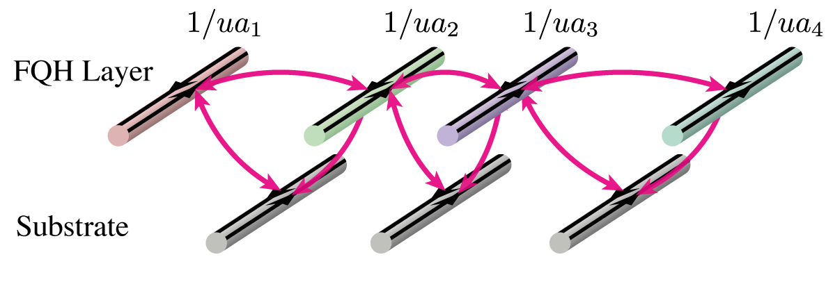
Figure S1: The first layer depicts a configuration of wires with each pair of wires hosting differently fractionalised quasiparticles, labelled as the fractional quantum Hall (FQH) layer. A second layer of un-fractionalised wires is added as a substrate, ensuring that all couplings respect charge conservation.

As discussed in Section III.2.1 the total charge of the system is not conserved when coupling two regions characterized by different fractional fillings [164, 165]. In this Appendix, we show that coupling the system to a substrate allows us to restore charge conservation while keeping the system gapped.

Consider the coupling between two regions with fractional coefficients $ua^{2}$ and $ub^{2}$ (with $a\neq b$). The corresponding coupling operator is given by Eq. (52), which we recall here for convenience:

$$\mathcal{O}(x)=\cos\left(b\varphi_{1}-a\varphi_{2}+ua^{2}b\theta_{1}+uab^{2}\theta_{2}\right).$$ (124)

Comparing this expression with Eq. 23, we can extract the values of $n_{1},n_{2},m_{1},m_{2}$, see Eqs. 7 and 8. According to the charge conservation condition Eq. 10, the net charge created or destroyed on each wire is $n_{j}$, and the total charge is conserved only if $n_{1}+n_{2}=0$. This condition is violated here, as $(b-a)$ charges are effectively added to or removed from the system, indicating a breakdown of charge conservation.

This issue can be resolved by introducing an additional substrate wire at the interface, serving as a charge reservoir. An example configuration is shown in Fig. S1. For fermions, $a$ and $b$ are odd, and hence $a-b$ is even, allowing for the symmetric placement of $(a-b)/2$ charges on right- and left-moving modes of the extra wire. Labelling the substrate wire with the subscript $\mathrm{sub}$, we assign $s_{\mathrm{sub}}^{R}=(a-b)/2$ and $s_{\mathrm{sub}}^{L}=(a-b)/2$, resulting in: $n_{\mathrm{sub}}=(a-b),m_{\mathrm{sub}}=0$.

The modified coupling operator, incorporating the substrate wire, becomes:

$$\begin{aligned} \mathcal{O}(x)=\cos\big{(}b\varphi_{1}&-a\varphi_{2}+(a-b)\varphi_{\mathrm{sub}}\\ &+ua^{2}b\theta_{1}+uab^{2}\theta_{2}\big{)}.\end{aligned}$$ (125)

Importantly, this expression only depends on the bosonic phase field $\varphi_{\mathrm{sub}}$, so the substrate wire remains non-fractionalised. The coupling always adds or removes an even number of fermions to the substrate, since $a-b$ is always even. Thus, the substrate may interpreted to be in a superconducting phase where charge is conserved modulo $a-b$ [102, 188, 189].

To satisfy momentum conservation must we must also fulfil the condition in Eq. (53)

$$B\left[by_{1}-ay_{2}+(a-b)y_{\mathrm{sub}}\right]+k_{F}uab(a+b)=0,$$ (126)

which can be rewritten as

$$B\left[b(y_{1}-y_{\mathrm{sub}})-a(y_{2}-y_{\mathrm{sub}})\right]+k_{F}uab(a+b)=0.$$ (127)

This condition simply reflects an origin shift, which can always be satisfied by appropriately positioning the wires.

Finally, since the field expressions associated with the fractional quantum Hall layer do not involve those of the substrate, the canonical commutation relations remain unchanged in its presence. Moreover, both the $\rho$ operator, propagating along a quasiwire and defined in  Eq. 95, and the $\chi$ operator, the tunnelling between neighbouring quasiwires defined in  Eq. 89, commute with the substrate fields and are thus unaffected by the substrate.

References

- Kitaev [2003] A. Kitaev, Fault-tolerant quantum computation by anyons, Annals of Physics 303, 2 (2003).
- Nayak et al. [2008] C. Nayak, S. H. Simon, A. Stern, M. Freedman, and S. Das Sarma, Non-Abelian anyons and topological quantum computation, Rev. Mod. Phys. 80, 1083 (2008).
- Wen [2007] X.-G. Wen, Quantum Field Theory of Many-Body Systems (Oxford University Press, 2007).
- Tsui et al. [1982] D. C. Tsui, H. L. Stormer, and A. C. Gossard, Two-Dimensional Magnetotransport in the Extreme Quantum Limit, Phys. Rev. Lett. 48, 1559 (1982).
- Laughlin [1983] R. B. Laughlin, Anomalous Quantum Hall Effect: An Incompressible Quantum Fluid with Fractionally Charged Excitations, Phys. Rev. Lett. 50, 1395 (1983).
- Sheng et al. [2003] D. N. Sheng, X. Wan, E. H. Rezayi, K. Yang, R. N. Bhatt, and F. D. M. Haldane, Disorder-Driven Collapse of the Mobility Gap and Transition to an Insulator in the Fractional Quantum Hall Effect, Physical Review Letters 90, 256802 (2003).
- Kane et al. [1994] C. L. Kane, M. P. A. Fisher, and J. Polchinski, Randomness at the edge: Theory of quantum Hall transport at filling =2/3, Phys. Rev. Lett. 72, 4129 (1994).
- Kane and Fisher [1995] C. L. Kane and M. P. A. Fisher, Impurity scattering and transport of fractional quantum Hall edge states, Phys. Rev. B 51, 13449 (1995).
- Haldane [1995] F. D. M. Haldane, Stability of Chiral Luttinger Liquids and Abelian Quantum Hall States, Phys. Rev. Lett. 74, 2090 (1995).
- Kao et al. [1999] H.-c. Kao, C.-H. Chang, and X.-G. Wen, Binding Transition in Quantum Hall Edge States, Phys. Rev. Lett. 83, 5563 (1999).
- Yutushui et al. [2024] M. Yutushui, J. Park, and A. D. Mirlin, Localization and conductance in fractional quantum Hall edges, Phys. Rev. B 110, 035402 (2024).
- Simon [2023] S. H. Simon, Topological Quantum (Oxford University Press, New York, 2023).
- Manna et al. [2020] S. Manna, B. Pal, W. Wang, and A. E. B. Nielsen, Anyons and fractional quantum Hall effect in fractal dimensions, Phys. Rev. Res. 2, 023401 (2020).
- Manna et al. [2022a] S. Manna, C. W. Duncan, C. A. Weidner, J. F. Sherson, and A. E. B. Nielsen, Anyon braiding on a fractal lattice with a local Hamiltonian, Phys. Rev. A 105, L021302 (2022a).
- Manna et al. [2023] S. Manna, C. W. Duncan, C. A. Weidner, J. F. Sherson, and A. E. B. Nielsen, Erratum: Anyon braiding on a fractal lattice with a local Hamiltonian [Phys. Rev. A 105, L021302 (2022)], Phys. Rev. A 107, 069901 (2023).
- Li et al. [2022a] X. Li, M. C. Jha, and A. E. B. Nielsen, Laughlin topology on fractal lattices without area law entanglement, Phys. Rev. B 105, 085152 (2022a).
- Jha and Nielsen [2023] M. C. Jha and A. E. B. Nielsen, Properties of Laughlin states on fractal lattices, Journal of Statistical Mechanics: Theory and Experiment 2023, 053103 (2023).
- Jaworowski et al. [2023] B. d. z. Jaworowski, M. Iversen, and A. E. B. Nielsen, Approximate Hofstadter- and Kapit-Mueller-like parent Hamiltonians for Laughlin states on fractals, Phys. Rev. A 107, 063315 (2023).
- Duncan et al. [2020] C. W. Duncan, S. Manna, and A. E. B. Nielsen, Topological models in rotationally symmetric quasicrystals, Phys. Rev. B 101, 115413 (2020).
- Cai et al. [2023] J. Cai, E. Anderson, C. Wang, X. Zhang, X. Liu, W. Holtzmann, Y. Zhang, F. Fan, T. Taniguchi, K. Watanabe, Y. Ran, T. Cao, L. Fu, D. Xiao, W. Yao, and X. Xu, Signatures of fractional quantum anomalous Hall states in twisted MoTe2, Nature 622, 63 (2023).
- Zeng et al. [2023] Y. Zeng, Z. Xia, K. Kang, J. Zhu, P. Knüppel, C. Vaswani, K. Watanabe, T. Taniguchi, K. F. Mak, and J. Shan, Thermodynamic evidence of fractional Chern insulator in moiré MoTe2, Nature 622, 69 (2023).
- Park et al. [2023] H. Park, J. Cai, E. Anderson, Y. Zhang, J. Zhu, X. Liu, C. Wang, W. Holtzmann, C. Hu, Z. Liu, T. Taniguchi, K. Watanabe, J.-H. Chu, T. Cao, L. Fu, W. Yao, C.-Z. Chang, D. Cobden, D. Xiao, and X. Xu, Observation of fractionally quantized anomalous Hall effect, Nature 622, 74 (2023).
- Xu et al. [2023] F. Xu, Z. Sun, T. Jia, C. Liu, C. Xu, C. Li, Y. Gu, K. Watanabe, T. Taniguchi, B. Tong, J. Jia, Z. Shi, S. Jiang, Y. Zhang, X. Liu, and T. Li, Observation of Integer and Fractional Quantum Anomalous Hall Effects in Twisted Bilayer MoTe2, Phys. Rev. X 13, 031037 (2023).
- Kang et al. [2024] K. Kang, B. Shen, Y. Qiu, Y. Zeng, Z. Xia, K. Watanabe, T. Taniguchi, J. Shan, and K. F. Mak, Evidence of the fractional quantum spin Hall effect in moiré MoTe2, Nature 628, 522 (2024).
- Lu et al. [2024] Z. Lu, T. Han, Y. Yao, A. P. Reddy, J. Yang, J. Seo, K. Watanabe, T. Taniguchi, L. Fu, and L. Ju, Fractional quantum anomalous Hall effect in multilayer graphene, Nature 626, 759 (2024).
- Xie et al. [2024] J. Xie, Z. Huo, X. Lu, Z. Feng, Z. Zhang, W. Wang, Q. Yang, K. Watanabe, T. Taniguchi, K. Liu, Z. Song, X. C. Xie, J. Liu, and X. Lu, Even- and Odd-denominator Fractional Quantum Anomalous Hall Effect in Graphene Moiré Superlattices, Preprint at https://arxiv.org/abs/2405.16944 (2024).
- Waters et al. [2024] D. Waters, A. Okounkova, R. Su, B. Zhou, J. Yao, K. Watanabe, T. Taniguchi, X. Xu, Y.-H. Zhang, J. Folk, and M. Yankowitz, Interplay of electronic crystals with integer and fractional Chern insulators in moiré pentalayer graphene, Preprint at https://arxiv.org/abs/22408.10133 (2024).
- Lu et al. [2024] Z. Lu, T. Han, Y. Yao, J. Yang, J. Seo, L. Shi, S. Ye, K. Watanabe, T. Taniguchi, and L. Ju, Extended Quantum Anomalous Hall States in Graphene/hBN Moiré Superlattices, Preprint at https://arxiv.org/abs/2408.10203 (2024).
- Neupert et al. [2011] T. Neupert, L. Santos, C. Chamon, and C. Mudry, Fractional Quantum Hall States at Zero Magnetic Field, Phys. Rev. Lett. 106, 236804 (2011).
- Tang et al. [2011] E. Tang, J.-W. Mei, and X.-G. Wen, High-Temperature Fractional Quantum Hall States, Phys. Rev. Lett. 106, 236802 (2011).
- Sun et al. [2011] K. Sun, Z. Gu, H. Katsura, and S. Das Sarma, Nearly Flatbands with Nontrivial Topology, Phys. Rev. Lett. 106, 236803 (2011).
- Sheng et al. [2011] D. N. Sheng, Z.-C. Gu, K. Sun, and L. Sheng, Fractional quantum Hall effect in the absence of Landau levels, Nature Communications 2, 389 (2011).
- Regnault and Bernevig [2011] N. Regnault and B. A. Bernevig, Fractional Chern Insulator, Phys. Rev. X 1, 021014 (2011).
- Grushin and Repellin [2023] A. G. Grushin and C. Repellin, Amorphous and Polycrystalline Routes toward a Chiral Spin Liquid, Phys. Rev. Lett. 130, 186702 (2023).
- Cassella et al. [2023] G. Cassella, P. d’Ornellas, T. Hodson, W. M. H. Natori, and J. Knolle, An exact chiral amorphous spin liquid, Nature Communications 14, 6663 (2023).
- Kraus et al. [2012] Y. E. Kraus, Y. Lahini, Z. Ringel, M. Verbin, and O. Zilberberg, Topological States and Adiabatic Pumping in Quasicrystals, Physical Review Letters 109, 106402 (2012).
- Tran et al. [2015] D. T. Tran, A. Dauphin, N. Goldman, and P. Gaspard, Topological Hofstadter insulators in a two-dimensional quasicrystal, Physical Review B 91, 085125 (2015).
- Bandres et al. [2016] M. A. Bandres, M. C. Rechtsman, and M. Segev, Topological Photonic Quasicrystals: Fractal Topological Spectrum and Protected Transport, Physical Review X 6, 011016 (2016).
- Fuchs and Vidal [2016] J.-N. Fuchs and J. Vidal, Hofstadter butterfly of a quasicrystal, Physical Review B 94, 205437 (2016).
- Huang and Liu [2018] H. Huang and F. Liu, Theory of spin Bott index for quantum spin Hall states in nonperiodic systems, Phys. Rev. B 98, 125130 (2018).
- Fuchs et al. [2018] J.-N. Fuchs, R. Mosseri, and J. Vidal, Landau levels in quasicrystals, Physical Review B 98, 145 (2018).
- Loring [2019] T. A. Loring, Bulk spectrum and K-theory for infinite-area topological quasicrystals, Journal of Mathematical Physics 60, 081903 (2019).
- Varjas et al. [2019] D. Varjas, A. Lau, K. Pöyhönen, A. R. Akhmerov, D. I. Pikulin, and I. C. Fulga, Topological Phases without Crystalline Counterparts, Phys. Rev. Lett. 123, 196401 (2019).
- Chen et al. [2019] R. Chen, D.-H. Xu, and B. Zhou, Topological Anderson insulator phase in a quasicrystal lattice, Phys. Rev. B 100, 115311 (2019).
- He et al. [2019] A.-L. He, L.-R. Ding, Y. Zhou, Y.-F. Wang, and C.-D. Gong, Quasicrystalline Chern insulators, Phys. Rev. B 100, 214109 (2019).
- Zilberberg [2021] O. Zilberberg, Topology in quasicrystals, Opt. Mater. Express 11, 1143 (2021).
- Hua et al. [2021] C.-B. Hua, Z.-R. Liu, T. Peng, R. Chen, D.-H. Xu, and B. Zhou, Disorder-induced chiral and helical Majorana edge modes in a two-dimensional Ammann-Beenker quasicrystal, Phys. Rev. B 104, 155304 (2021).
- Jeon et al. [2022] J. Jeon, M. J. Park, and S. Lee, Length scale formation in the Landau levels of quasicrystals, Phys. Rev. B 105, 045146 (2022).
- Schirmann et al. [2024] J. Schirmann, S. Franca, F. Flicker, and A. G. Grushin, Physical Properties of an Aperiodic Monotile with Graphene-like Features, Chirality, and Zero Modes, Phys. Rev. Lett. 132, 086402 (2024).
- Agarwala and Shenoy [2017] A. Agarwala and V. B. Shenoy, Topological Insulators in Amorphous Systems, Phys. Rev. Lett. 118, 236402 (2017).
- Mansha and Chong [2017] S. Mansha and Y. D. Chong, Robust edge states in amorphous gyromagnetic photonic lattices, Phys. Rev. B 96, 121405 (2017).
- Xiao and Fan [2017] M. Xiao and S. Fan, Photonic Chern insulator through homogenization of an array of particles, Phys. Rev. B 96, 100202 (2017).
- Mitchell et al. [2018] N. P. Mitchell, L. M. Nash, D. Hexner, A. M. Turner, and W. T. M. Irvine, Amorphous topological insulators constructed from random point sets, Nature Physics 14, 380 (2018).
- Bourne and Prodan [2018] C. Bourne and E. Prodan, Non-commutative Chern numbers for generic aperiodic discrete systems, Journal of Physics A: Mathematical and Theoretical 51, 235202 (2018).
- Pöyhönen et al. [2018] K. Pöyhönen, I. Sahlberg, A. Westström, and T. Ojanen, Amorphous topological superconductivity in a Shiba glass, Nature Communications 9, 2103 (2018).
- Minarelli et al. [2019] E. L. Minarelli, K. Pöyhönen, G. A. R. van Dalum, T. Ojanen, and L. Fritz, Engineering of Chern insulators and circuits of topological edge states, Physical Review B 99, 165413 (2019).
- Chern [2019] G.-W. Chern, Topological insulator in an atomic liquid, Europhysics Letters 126, 37002 (2019).
- Mano and Ohtsuki [2019] T. Mano and T. Ohtsuki, Application of Convolutional Neural Network to Quantum Percolation in Topological Insulators, Journal of the Physical Society of Japan 88, 123704 (2019).
- Corbae et al. [2023a] P. Corbae, S. Ciocys, D. Varjas, E. Kennedy, S. Zeltmann, M. Molina-Ruiz, S. M. Griffin, C. Jozwiak, Z. Chen, L.-W. Wang, A. M. Minor, M. Scott, A. G. Grushin, A. Lanzara, and F. Hellman, Observation of spin-momentum locked surface states in amorphous Bi2Se3, Nature Materials 22, 200 (2023a).
- Costa et al. [2019] M. Costa, G. R. Schleder, M. Buongiorno Nardelli, C. Lewenkopf, and A. Fazzio, Toward Realistic Amorphous Topological Insulators, Nano Letters 19, 8941 (2019).
- Marsal et al. [2020] Q. Marsal, D. Varjas, and A. G. Grushin, Topological Weaire–Thorpe models of amorphous matter, Proceedings of the National Academy of Sciences 117, 30260 (2020).
- Sahlberg et al. [2020] I. Sahlberg, A. Westström, K. Pöyhönen, and T. Ojanen, Topological phase transitions in glassy quantum matter, Phys. Rev. Res. 2, 013053 (2020).
- Ivaki et al. [2020] M. N. Ivaki, I. Sahlberg, and T. Ojanen, Criticality in amorphous topological matter: Beyond the universal scaling paradigm, Physical Review Research 2, 043301 (2020).
- Agarwala et al. [2020] A. Agarwala, V. Juričić, and B. Roy, Higher-order topological insulators in amorphous solids, Physical Review Research 2, 012067 (2020).
- Grushin [2022] A. G. Grushin, Topological phases of amorphous matter, in Low-Temperature Thermal and Vibrational Properties of Disordered Solids, edited by M. A. Ramos (World Scientific, 2022) Chap. 11.
- Wang et al. [2021] J.-H. Wang, Y.-B. Yang, N. Dai, and Y. Xu, Structural-Disorder-Induced Second-Order Topological Insulators in Three Dimensions, Physical Review Letters 126, 206404 (2021).
- Corbae et al. [2021] P. Corbae, F. Hellman, and S. M. Griffin, Structural disorder-driven topological phase transition in noncentrosymmetric BiTeI, Phys. Rev. B 103, 214203 (2021).
- Focassio et al. [2021] B. Focassio, G. R. Schleder, M. Costa, A. Fazzio, and C. Lewenkopf, Structural and electronic properties of realistic two-dimensional amorphous topological insulators, 2D Materials 8, 025032 (2021).
- Mitchell et al. [2021] N. P. Mitchell, A. M. Turner, and W. T. M. Irvine, Real-space origin of topological band gaps, localization, and reentrant phase transitions in gyroscopic metamaterials, Physical Review E 104, 025007 (2021).
- Spring et al. [2021] H. Spring, A. Akhmerov, and D. Varjas, Amorphous topological phases protected by continuous rotation symmetry, SciPost Physics 11, 022 (2021).
- Wang et al. [2022] C. Wang, T. Cheng, Z. Liu, F. Liu, and H. Huang, Structural Amorphization-Induced Topological Order, Physical Review Letters 128, 056401 (2022).
- Marsal et al. [2023] Q. Marsal, D. Varjas, and A. G. Grushin, Obstructed insulators and flat bands in topological phase-change materials, Phys. Rev. B 107, 045119 (2023).
- Peng et al. [2022] T. Peng, C.-B. Hua, R. Chen, Z.-R. Liu, H.-M. Huang, and B. Zhou, Density-driven higher-order topological phase transitions in amorphous solids, Phys. Rev. B 106, 125310 (2022).
- Uría-Álvarez et al. [2022] A. J. Uría-Álvarez, D. Molpeceres-Mingo, and J. J. Palacios, Deep learning for disordered topological insulators through their entanglement spectrum, Phys. Rev. B 105, 155128 (2022).
- Muñoz Segovia et al. [2023] D. Muñoz Segovia, P. Corbae, D. Varjas, F. Hellman, S. M. Griffin, and A. G. Grushin, Structural spillage: An efficient method to identify noncrystalline topological materials, Phys. Rev. Res. 5, L042011 (2023).
- Corbae et al. [2023b] P. Corbae, J. D. Hannukainen, Q. Marsal, D. Muñoz-Segovia, and A. G. Grushin, Amorphous topological matter: Theory and experiment, Europhysics Letters 142, 16001 (2023b).
- Manna et al. [2024a] S. Manna, S. K. Das, and B. Roy, Noncrystalline topological superconductors, Phys. Rev. B 109, 174512 (2024a).
- Ciocys et al. [2024] S. T. Ciocys, Q. Marsal, P. Corbae, D. Varjas, E. Kennedy, M. Scott, F. Hellman, A. G. Grushin, and A. Lanzara, Establishing coherent momentum-space electronic states in locally ordered materials, Nature Communications 15, 8141 (2024).
- Ur´ıa-Álvarez and Palacios [2024] A. Uría-Álvarez and J. Palacios, Amorphization-induced topological and insulator-metal transitions in bidimensional BixSb1-x alloys, Preprint at https://arxiv.org/abs/2410.16034 (2024).
- Brzezińska et al. [2018] M. Brzezińska, A. M. Cook, and T. Neupert, Topology in the Sierpiński-Hofstadter problem, Phys. Rev. B 98, 205116 (2018).
- Pai and Prem [2019] S. Pai and A. Prem, Topological states on fractal lattices, Phys. Rev. B 100, 155135 (2019).
- Iliasov et al. [2020] A. A. Iliasov, M. I. Katsnelson, and S. Yuan, Hall conductivity of a Sierpiński carpet, Phys. Rev. B 101, 045413 (2020).
- Fremling et al. [2020] M. Fremling, M. van Hooft, C. M. Smith, and L. Fritz, Existence of robust edge currents in Sierpiński fractals, Phys. Rev. Res. 2, 013044 (2020).
- Yang et al. [2020] Z. Yang, E. Lustig, Y. Lumer, and M. Segev, Photonic Floquet topological insulators in a fractal lattice, Light: Science & Applications 9, 128 (2020).
- Manna et al. [2024b] S. Manna, S. K. Das, and B. Roy, Noncrystalline topological superconductors, Phys. Rev. B 109, 174512 (2024b).
- Manna and Roy [2023] S. Manna and B. Roy, Inner skin effects on non-Hermitian topological fractals, Communications Physics 6, 10 (2023).
- Li et al. [2022b] J. Li, Q. Mo, J.-H. Jiang, and Z. Yang, Higher-order topological phase in an acoustic fractal lattice, Science Bulletin 67, 2040 (2022b).
- Zheng et al. [2022] S. Zheng, X. Man, Z.-L. Kong, Z.-K. Lin, G. Duan, N. Chen, D. Yu, J.-H. Jiang, and B. Xia, Observation of fractal higher-order topological states in acoustic metamaterials, Science Bulletin 67, 2069 (2022).
- Biesenthal et al. [2022] T. Biesenthal, L. J. Maczewsky, Z. Yang, M. Kremer, M. Segev, A. Szameit, and M. Heinrich, Fractal photonic topological insulators, Science 376, 1114 (2022).
- Ivaki et al. [2022] M. N. Ivaki, I. Sahlberg, K. Pöyhönen, and T. Ojanen, Topological random fractals, Communications Physics 5, 327 (2022).
- Manna et al. [2022b] S. Manna, S. Nandy, and B. Roy, Higher-order topological phases on fractal lattices, Phys. Rev. B 105, L201301 (2022b).
- Ren et al. [2023] B. Ren, Y. V. Kartashov, L. J. Maczewsky, M. S. Kirsch, H. Wang, A. Szameit, M. Heinrich, and Y. Zhang, Theory of nonlinear corner states in photonic fractal lattices, Nanophotonics 12, 3829 (2023).
- Salib et al. [2024] D. J. Salib, A. J. Mains, and B. Roy, Topological insulators on fractal lattices: A general principle of construction, Phys. Rev. B 110, L241302 (2024).
- Lai et al. [2024] P. Lai, H. Liu, B. Xie, W. Deng, H. Wang, H. Cheng, Z. Liu, and S. Chen, Spin Chern insulator in a phononic fractal lattice, Phys. Rev. B 109, L140104 (2024).
- Canyellas et al. [2024] R. Canyellas, C. Liu, R. Arouca, L. Eek, G. Wang, Y. Yin, D. Guan, Y. Li, S. Wang, H. Zheng, C. Liu, J. Jia, and C. Morais Smith, Topological edge and corner states in bismuth fractal nanostructures, Nature Physics 20, 1421 (2024).
- Li and Yan [2024] Z. Li and P. Yan, Peculiar corner states in magnetic fractals, Phys. Rev. B 110, 024402 (2024).
- Lage et al. [2024] L. L. Lage, N. C. Rappe, and A. Latgé, Corner and edge states in topological Sierpinski Carpet systems, Journal of Physics: Condensed Matter 37, 025303 (2024).
- Emery et al. [2000] V. J. Emery, E. Fradkin, S. A. Kivelson, and T. C. Lubensky, Quantum Theory of the Smectic Metal State in Stripe Phases, Phys. Rev. Lett. 85, 2160 (2000).
- Vishwanath and Carpentier [2001] A. Vishwanath and D. Carpentier, Two-Dimensional Anisotropic Non-Fermi-Liquid Phase of Coupled Luttinger Liquids, Phys. Rev. Lett. 86, 676 (2001).
- Mukhopadhyay et al. [2001a] R. Mukhopadhyay, C. L. Kane, and T. C. Lubensky, Sliding Luttinger liquid phases, Phys. Rev. B 64, 045120 (2001a).
- Mukhopadhyay et al. [2001b] R. Mukhopadhyay, C. L. Kane, and T. C. Lubensky, Crossed sliding Luttinger liquid phase, Phys. Rev. B 63, 081103 (2001b).
- Kane et al. [2002] C. L. Kane, R. Mukhopadhyay, and T. C. Lubensky, Fractional Quantum Hall Effect in an Array of Quantum Wires, Phys. Rev. Lett. 88, 036401 (2002).
- Teo and Kane [2014] J. C. Y. Teo and C. L. Kane, From Luttinger liquid to non-Abelian quantum Hall states, Phys. Rev. B 89, 085101 (2014).
- Tam and Kane [2021] P. M. Tam and C. L. Kane, Nondiagonal anisotropic quantum Hall states, Phys. Rev. B 103, 035142 (2021).
- Tam et al. [2020] P. M. Tam, Y. Hu, and C. L. Kane, Coupled wire model of orbifold quantum hall states, Phys. Rev. B 101, 125104 (2020).
- Tam et al. [2022] P. M. Tam, J. W. F. Venderbos, and C. L. Kane, Toric-code insulator enriched by translation symmetry, Phys. Rev. B 105, 045106 (2022).
- Clarke et al. [2013] D. J. Clarke, J. Alicea, and K. Shtengel, Exotic non-Abelian anyons from conventional fractional quantum Hall states, Nature Communications 4, 1348 (2013).
- Neupert et al. [2014] T. Neupert, C. Chamon, C. Mudry, and R. Thomale, Wire deconstructionism of two-dimensional topological phases, Phys. Rev. B 90, 205101 (2014).
- Klinovaja and Loss [2014] J. Klinovaja and D. Loss, Integer and fractional quantum Hall effect in a strip of stripes, The European Physical Journal B 87, 171 (2014).
- Oreg et al. [2014] Y. Oreg, E. Sela, and A. Stern, Fractional helical liquids in quantum wires, Phys. Rev. B 89, 115402 (2014).
- Sagi and Oreg [2014] E. Sagi and Y. Oreg, Non-Abelian topological insulators from an array of quantum wires, Phys. Rev. B 90, 201102 (2014).
- Santos et al. [2015] R. A. Santos, C.-W. Huang, Y. Gefen, and D. B. Gutman, Fractional topological insulators: From sliding Luttinger liquids to Chern-Simons theory, Phys. Rev. B 91, 205141 (2015).
- Cano et al. [2015] J. Cano, T. L. Hughes, and M. Mulligan, Interactions along an entanglement cut in abelian topological phases, Phys. Rev. B 92, 075104 (2015).
- Klinovaja et al. [2015] J. Klinovaja, Y. Tserkovnyak, and D. Loss, Integer and fractional quantum anomalous Hall effect in a strip of stripes model, Phys. Rev. B 91, 085426 (2015).
- Sagi and Oreg [2015] E. Sagi and Y. Oreg, From an array of quantum wires to three-dimensional fractional topological insulators, Phys. Rev. B 92, 195137 (2015).
- Sagi et al. [2015] E. Sagi, Y. Oreg, A. Stern, and B. I. Halperin, Imprint of topological degeneracy in quasi-one-dimensional fractional quantum Hall states, Phys. Rev. B 91, 245144 (2015).
- Meng [2015] T. Meng, Fractional topological phases in three-dimensional coupled-wire systems, Phys. Rev. B 92, 115152 (2015).
- Meng et al. [2016] T. Meng, A. G. Grushin, K. Shtengel, and J. H. Bardarson, Theory of a D fractional chiral metal: Interacting variant of the Weyl semimetal, Phys. Rev. B 94, 155136 (2016).
- Mross et al. [2016] D. F. Mross, J. Alicea, and O. I. Motrunich, Explicit Derivation of Duality between a Free Dirac Cone and Quantum Electrodynamics in () Dimensions, Phys. Rev. Lett. 117, 016802 (2016).
- Iadecola et al. [2016] T. Iadecola, T. Neupert, C. Chamon, and C. Mudry, Wire constructions of Abelian topological phases in three or more dimensions, Phys. Rev. B 93, 195136 (2016).
- Fuji et al. [2016] Y. Fuji, Y.-C. He, S. Bhattacharjee, and F. Pollmann, Bridging coupled wires and lattice Hamiltonian for two-component bosonic quantum Hall states, Phys. Rev. B 93, 195143 (2016).
- Sagi et al. [2017a] E. Sagi, A. Haim, E. Berg, F. von Oppen, and Y. Oreg, Fractional chiral superconductors, Phys. Rev. B 96, 235144 (2017a).
- Kane et al. [2017] C. L. Kane, A. Stern, and B. I. Halperin, Pairing in Luttinger Liquids and Quantum Hall States, Phys. Rev. X 7, 031009 (2017).
- Park et al. [2018] M. J. Park, S. Raza, M. J. Gilbert, and J. C. Y. Teo, Coupled wire models of interacting Dirac nodal superconductors, Phys. Rev. B 98, 184514 (2018).
- Kane and Stern [2018] C. L. Kane and A. Stern, Coupled wire model of orbifold quantum Hall states, Phys. Rev. B 98, 085302 (2018).
- Fuji and Furusaki [2019] Y. Fuji and A. Furusaki, Quantum Hall hierarchy from coupled wires, Phys. Rev. B 99, 035130 (2019).
- Laubscher et al. [2019] K. Laubscher, D. Loss, and J. Klinovaja, Fractional topological superconductivity and parafermion corner states, Phys. Rev. Res. 1, 032017 (2019).
- Bardyn et al. [2019] C.-E. Bardyn, M. Filippone, and T. Giamarchi, Bulk pumping in two-dimensional topological phases, Phys. Rev. B 99, 035150 (2019).
- Imamura et al. [2019a] Y. Imamura, K. Totsuka, and T. H. Hansson, From coupled-wire construction of quantum Hall states to wave functions and hydrodynamics, Phys. Rev. B 100, 125148 (2019a).
- Han and Teo [2019] B. Han and J. C. Y. Teo, Coupled-wire description of surface topological order, Phys. Rev. B 99, 235102 (2019).
- Meng [2020] T. Meng, Coupled-wire constructions: a Luttinger liquid approach to topology, The European Physical Journal Special Topics 229, 527 (2020).
- Crépel et al. [2020] V. Crépel, B. Estienne, and N. Regnault, Microscopic study of the coupled-wire construction and plausible realization in spin-dependent optical lattices, Phys. Rev. B 101, 235158 (2020).
- Laubscher et al. [2020] K. Laubscher, D. Loss, and J. Klinovaja, Majorana and parafermion corner states from two coupled sheets of bilayer graphene, Phys. Rev. Res. 2, 013330 (2020).
- Li et al. [2020] C. Li, H. Ebisu, S. Sahoo, Y. Oreg, and M. Franz, Coupled wire construction of a topological phase with chiral tricritical Ising edge modes, Phys. Rev. B 102, 165123 (2020).
- Laubscher et al. [2021] K. Laubscher, C. S. Weber, D. M. Kennes, M. Pletyukhov, H. Schoeller, D. Loss, and J. Klinovaja, Fractional boundary charges with quantized slopes in interacting one- and two-dimensional systems, Phys. Rev. B 104, 035432 (2021).
- Zhang [2022] J.-H. Zhang, Strongly correlated crystalline higher-order topological phases in two-dimensional systems: A coupled-wire study, Phys. Rev. B 106, L020503 (2022).
- Laubscher et al. [2023] K. Laubscher, P. Keizer, and J. Klinovaja, Fractional second-order topological insulator from a three-dimensional coupled-wires construction, Phys. Rev. B 107, 045409 (2023).
- Pinchenkova et al. [2025] V. Pinchenkova, K. Laubscher, and J. Klinovaja, Fractional chiral second-order topological insulator from a three-dimensional array of coupled wires, Preprint at https://arxiv.org/abs/2504.06101 (2025).
- Meng et al. [2015] T. Meng, T. Neupert, M. Greiter, and R. Thomale, Coupled-wire construction of chiral spin liquids, Phys. Rev. B 91, 241106 (2015).
- Gorohovsky et al. [2015] G. Gorohovsky, R. G. Pereira, and E. Sela, Chiral spin liquids in arrays of spin chains, Phys. Rev. B 91, 245139 (2015).
- Patel and Chowdhury [2016] A. A. Patel and D. Chowdhury, Two-dimensional spin liquids with topological order in an array of quantum wires, Phys. Rev. B 94, 195130 (2016).
- Huang et al. [2016] P.-H. Huang, J.-H. Chen, P. R. S. Gomes, T. Neupert, C. Chamon, and C. Mudry, Non-Abelian topological spin liquids from arrays of quantum wires or spin chains, Phys. Rev. B 93, 205123 (2016).
- Lecheminant and Tsvelik [2017] P. Lecheminant and A. M. Tsvelik, Lattice spin models for non-Abelian chiral spin liquids, Phys. Rev. B 95, 140406 (2017).
- Pereira and Bieri [2018] R. G. Pereira and S. Bieri, Gapless chiral spin liquid from coupled chains on the kagome lattice, SciPost Phys. 4, 004 (2018).
- Ferraz et al. [2019] G. Ferraz, F. B. Ramos, R. Egger, and R. G. Pereira, Spin Chain Network Construction of Chiral Spin Liquids, Phys. Rev. Lett. 123, 137202 (2019).
- Slagle et al. [2022] K. Slagle, Y. Liu, D. Aasen, H. Pichler, R. S. K. Mong, X. Chen, M. Endres, and J. Alicea, Quantum spin liquids bootstrapped from Ising criticality in Rydberg arrays, Phys. Rev. B 106, 115122 (2022).
- Mondal et al. [2023] S. Mondal, A. Agarwala, T. Mishra, and A. Prakash, Symmetry-enriched criticality in a coupled spin ladder, Phys. Rev. B 108, 245135 (2023).
- Gao et al. [2025] T. Gao, N. Tausendpfund, E. L. Weerda, M. Rizzi, and D. F. Mross, Triangular lattice models of the Kalmeyer-Laughlin spin liquid from coupled wires, Preprint at https://arxiv.org/abs/2502.13223 (2025).
- Halász et al. [2017] G. B. Halász, T. H. Hsieh, and L. Balents, Fracton Topological Phases from Strongly Coupled Spin Chains, Phys. Rev. Lett. 119, 257202 (2017).
- Leviatan and Mross [2020] E. Leviatan and D. F. Mross, Unification of parton and coupled-wire approaches to quantum magnetism in two dimensions, Phys. Rev. Res. 2, 043437 (2020).
- Sullivan et al. [2021] J. Sullivan, A. Dua, and M. Cheng, Fractonic topological phases from coupled wires, Phys. Rev. Res. 3, 023123 (2021).
- May-Mann et al. [2022] J. May-Mann, Y. You, T. L. Hughes, and Z. Bi, Interaction-enabled fractonic higher-order topological phases, Phys. Rev. B 105, 245122 (2022).
- Fuji and Furusaki [2023] Y. Fuji and A. Furusaki, Bridging three-dimensional coupled-wire models and cellular topological states: Solvable models for topological and fracton orders, Phys. Rev. Res. 5, 043108 (2023).
- You et al. [2025] Y. You, J. Bibo, T. L. Hughes, and F. Pollmann, Fractonic critical point proximate to a higher-order topological insulator: A Coupled wire approach, Annals of Physics 474, 169927 (2025).
- Wu et al. [2019] X.-C. Wu, C.-M. Jian, and C. Xu, Coupled-wire description of the correlated physics in twisted bilayer graphene, Phys. Rev. B 99, 161405 (2019).
- Chou et al. [2019] Y.-Z. Chou, Y.-P. Lin, S. Das Sarma, and R. M. Nandkishore, Superconductor versus insulator in twisted bilayer graphene, Phys. Rev. B 100, 115128 (2019).
- Chen et al. [2020] C. Chen, A. H. Castro Neto, and V. M. Pereira, Correlated states of a triangular net of coupled quantum wires: Implications for the phase diagram of marginally twisted bilayer graphene, Phys. Rev. B 101, 165431 (2020).
- Chou et al. [2021] Y.-Z. Chou, F. Wu, and J. D. Sau, Charge density wave and finite-temperature transport in minimally twisted bilayer graphene, Phys. Rev. B 104, 045146 (2021).
- Lee et al. [2021] J. M. Lee, M. Oshikawa, and G. Y. Cho, Non-fermi liquids in conducting two-dimensional networks, Phys. Rev. Lett. 126, 186601 (2021).
- Hsu et al. [2023] C.-H. Hsu, D. Loss, and J. Klinovaja, General scattering and electronic states in a quantum-wire network of moiré systems, Phys. Rev. B 108, L121409 (2023).
- Hu et al. [2024a] Y. Hu, Y. Xu, and B. Lian, Twisted coupled wire model for a moiré sliding Luttinger liquid, Phys. Rev. B 110, L201106 (2024a).
- Shavit and Oreg [2024] G. Shavit and Y. Oreg, Quantum Geometry and Stabilization of Fractional Chern Insulators Far from the Ideal Limit, Phys. Rev. Lett. 133, 156504 (2024).
- Hu et al. [2024b] Y. Hu, Y. Xu, and B. Lian, Twisted coupled wire model for a moiré sliding Luttinger liquid, Phys. Rev. B 110, L201106 (2024b).
- Santos and Hughes [2017] L. H. Santos and T. L. Hughes, Parafermionic Wires at the Interface of Chiral Topological States, Phys. Rev. Lett. 118, 136801 (2017).
- May-Mann and Hughes [2019] J. May-Mann and T. L. Hughes, Families of gapped interfaces between fractional quantum Hall states, Phys. Rev. B 99, 155134 (2019).
- von Delft and Schoeller [1998] J. von Delft and H. Schoeller, Bosonization for beginners — refermionization for experts, Annalen der Physik 510, 225 (1998).
- Haldane [1981] F. D. M. Haldane, ’Luttinger liquid theory’ of one-dimensional quantum fluids. I. Properties of the Luttinger model and their extension to the general 1D interacting spinless Fermi gas, Journal of Physics C: Solid State Physics 14, 2585 (1981).
- Senechal [1999] D. Senechal, An introduction to bosonization, Preprint at https://arxiv.org/abs/cond-mat/9908262 (1999).
- [169] Of course, for fermionic systems we require odd, however the same can be done starting with bosons to obtain even fractions.
- Imamura et al. [2019b] Y. Imamura, K. Totsuka, and T. H. Hansson, From coupled-wire construction of quantum Hall states to wave functions and hydrodynamics, Phys. Rev. B 100, 125148 (2019b).
- Bézout [1779] E. Bézout, Théorie générale des équations algébriques, Manuscripta; History of science, 18th and 19th century (Ph.-D. Pierres, 1779).
- [172] To illustrate why the latter holds, consider the effect on and when .
- Nandkishore and Hermele [2019] R. M. Nandkishore and M. Hermele, Fractons, Annual Review of Condensed Matter Physics 10, 295–313 (2019).
- Pretko et al. [2020] M. Pretko, X. Chen, and Y. You, Fracton phases of matter, International Journal of Modern Physics A 35, 2030003 (2020).
- Martin et al. [2008] I. Martin, Y. M. Blanter, and A. F. Morpurgo, Topological Confinement in Bilayer Graphene, Phys. Rev. Lett. 100, 036804 (2008).
- Liu et al. [2019] X. Liu, Z. Hao, K. Watanabe, T. Taniguchi, B. I. Halperin, and P. Kim, Interlayer fractional quantum Hall effect in a coupled graphene double layer, Nature Physics 15, 893 (2019).
- Grivnin et al. [2014] A. Grivnin, H. Inoue, Y. Ronen, Y. Baum, M. Heiblum, V. Umansky, and D. Mahalu, Nonequilibrated counterpropagating edge modes in the fractional quantum hall regime, Phys. Rev. Lett. 113, 266803 (2014).
- Hashisaka et al. [2021] M. Hashisaka, T. Jonckheere, T. Akiho, S. Sasaki, J. Rech, T. Martin, and K. Muraki, Andreev reflection of fractional quantum hall quasiparticles, Nature Communications 12, 2794 (2021).
- Dutta et al. [2022] B. Dutta, W. Yang, R. Melcer, H. K. Kundu, M. Heiblum, V. Umansky, Y. Oreg, A. Stern, and D. Mross, Distinguishing between non-abelian topological orders in a quantum hall system, Science 375, 193 (2022).
- Cohen et al. [2023] L. A. Cohen, N. L. Samuelson, T. Wang, T. Taniguchi, K. Watanabe, M. P. Zaletel, and A. F. Young, Universal chiral Luttinger liquid behavior in a graphene fractional quantum Hall point contact, Science 382, 542 (2023).
- Hashisaka et al. [2023] M. Hashisaka, T. Ito, T. Akiho, S. Sasaki, N. Kumada, N. Shibata, and K. Muraki, Coherent-incoherent crossover of charge and neutral mode transport as evidence for the disorder-dominated fractional edge phase, Phys. Rev. X 13, 031024 (2023).
- Jaksch and Zoller [2003] D. Jaksch and P. Zoller, Creation of effective magnetic fields in optical lattices: the hofstadter butterfly for cold neutral atoms, New Journal of Physics 5, 56 (2003).
- Celi et al. [2014] A. Celi, P. Massignan, J. Ruseckas, N. Goldman, I. B. Spielman, G. Juzeliūnas, and M. Lewenstein, Synthetic gauge fields in synthetic dimensions, Phys. Rev. Lett. 112, 043001 (2014).
- Budich et al. [2017] J. C. Budich, A. Elben, M. Łkacki, A. Sterdyniak, M. A. Baranov, and P. Zoller, Coupled atomic wires in a synthetic magnetic field, Phys. Rev. A 95, 043632 (2017).
- Salerno et al. [2019] G. Salerno, H. M. Price, M. Lebrat, S. Häusler, T. Esslinger, L. Corman, J.-P. Brantut, and N. Goldman, Quantized hall conductance of a single atomic wire: A proposal based on synthetic dimensions, Phys. Rev. X 9, 041001 (2019).
- Zhou et al. [2023] T.-W. Zhou, G. Cappellini, D. Tusi, L. Franchi, J. Parravicini, C. Repellin, S. Greschner, M. Inguscio, T. Giamarchi, M. Filippone, J. Catani, and L. Fallani, Observation of universal Hall response in strongly interacting Fermions, Science 381, 427 (2023).
- Zhou et al. [2024] T. W. Zhou, T. Beller, G. Masini, J. Parravicini, G. Cappellini, C. Repellin, T. Giamarchi, J. Catani, M. Filippone, and L. Fallani, Measuring Hall voltage and Hall resistance in an atom-based quantum simulator, Preprint at https://arxiv.org/abs/2411.09744 (2024).
- Seroussi et al. [2014] I. Seroussi, E. Berg, and Y. Oreg, Topological superconducting phases of weakly coupled quantum wires, Phys. Rev. B 89, 104523 (2014).
- Sagi et al. [2017b] E. Sagi, A. Haim, E. Berg, F. von Oppen, and Y. Oreg, Fractional chiral superconductors, Phys. Rev. B 96, 235144 (2017b).