Instituto de Computação, Universidade Federal Fluminense, Brasil and http://www.ic.uff.br/˜lfignacio lfignacio@ic.uff.brhttps://orcid.org/0000-0002-3797-6053FAPERJ-JCNE (E-26/201.372/2022) and CNPq-Universal (406173/2021-4). LIRMM, Université de Montpellier, CNRS, France and https://www.lirmm.fr/˜sau/ ignasi.sau@lirmm.frhttps://orcid.org/0000-0002-8981-9287French project ELiT (ANR-20-CE48-0008-01). Instituto de Computação, Universidade Federal Fluminense, Brasil and IMPA - Instituto de Matemática Pura e Aplicada, Brasil and http://www.ic.uff.br/˜ueverton ueverton@ic.uff.brhttps://orcid.org/0000-0002-5320-9209CNPq (312344/2023-6), and FAPERJ (E-26/201.344/2021). Université de Lorraine, CNRS, Inria, LORIA, F-54000 Nancy, France and https://lipn.univ-paris13.fr/˜valenciapabon/ mario.valencia@loria.frhttps://orcid.org/0009-0006-0564-4341French project Abysm (ANR-23-CE48-0017). \CopyrightCunha, Sau, Souza, and Valencia-Pabon \ccsdesc[100]Theory of computation Parameterized complexity and exact algorithms; Mathematics of computing → Combinatorics. \relatedversionA conference version of this article will appear in the proceedings of ICALP 2025. We would like to thank the reviewers for their helpful remarks. \hideLIPIcs
Computing Distances on Graph Associahedra is Fixed-parameter Tractable
Abstract
An elimination tree of a connected graph is a rooted tree on the vertices of obtained by choosing a root and recursing on the connected components of to obtain the subtrees of . The graph associahedron of is a polytope whose vertices correspond to elimination trees of and whose edges correspond to tree rotations, a natural operation between elimination trees. These objects generalize associahedra, which correspond to the case where is a path. Ito et al. [ICALP 2023] recently proved that the problem of computing distances on graph associahedra is NP-hard. In this paper we prove that the problem, for a general graph , is fixed-parameter tractable parameterized by the distance . Prior to our work, only the case where is a path was known to be fixed-parameter tractable. To prove our result, we use a novel approach based on a marking scheme that restricts the search to a set of vertices whose size is bounded by a (large) function of .
keywords:
graph associahedra, elimination tree, rotation distance, parameterized complexity, fixed-parameter tractable algorithm, combinatorial shortest path, reconfiguration.1 Introduction
Given a connected and undirected graph , an elimination tree of is any rooted tree that can be defined recursively as follows. If , then consists of a single root vertex . Otherwise, a vertex is chosen as the root of , and an elimination tree is created for each connected component of . Each root of these elimination trees of is a child of in . For a disconnected graph , an elimination forest of is the disjoint union of elimination trees of the connected components of . Equivalently, an elimination forest of a graph is a rooted forest (that is, a forest with a root in every connected component) on vertex set such that for each edge , vertex is an ancestor of vertex in , or vice versa.
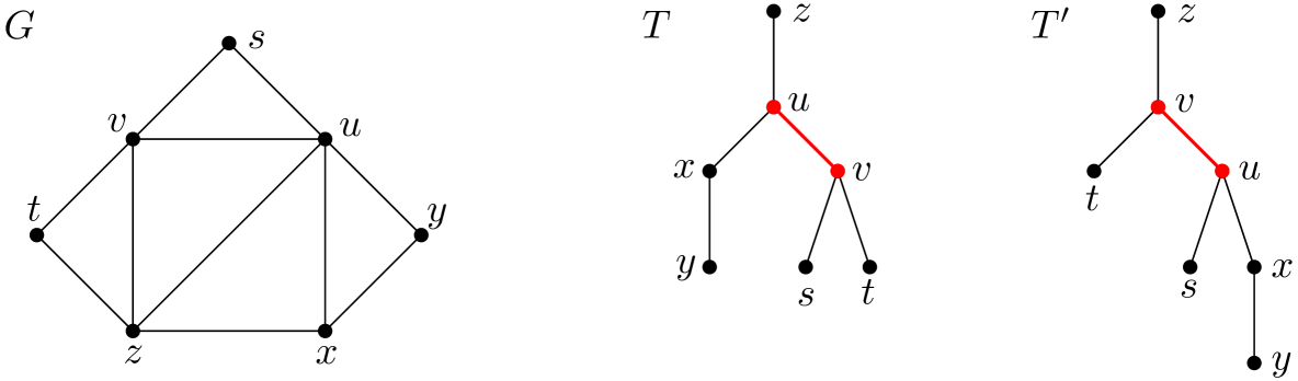
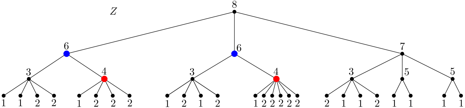
Figure 1 illustrates an example of two elimination trees and of a graph . With slight (and standard) abuse of notation, we use the same labels for the vertices of a graph and any of its elimination trees. Note that an elimination tree is unordered, i.e., there is no ordering associated with the children of a vertex in the tree. Similarly, there is no ordering among the elimination trees in an elimination forest.
Elimination trees have been studied extensively in various contexts, including graph theory, combinatorial optimization, polyhedral combinatorics, data structures, or VLSI design; see the recent paper by Cardinal, Merino, and Mütze [7] and the references therein. In particular, elimination trees play a prominent role in structural and algorithmic graph theory, as they appear naturally in several contexts. As a relevant example, the treedepth of a graph is defined as the minimum height of an elimination forest of [32].
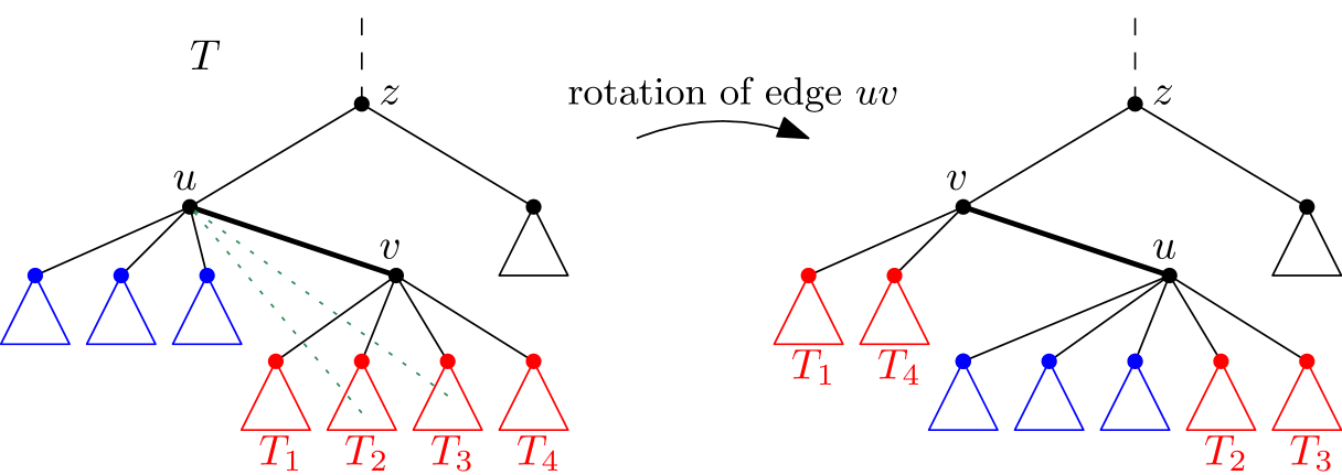
Given a class of combinatorial objects and a “local change” operation between them, the corresponding flip graph has as vertices the combinatorial objects, and its edges connect pairs of objects that differ by the prescribed change operation. In this article, we focus on the case where this class of combinatorial objects is the set of elimination forests of a graph . For these objects, the commonly considered “local change” operation is that of edge rotation defined as follows, where we suppose for simplicity that is connected. Given an elimination tree of a graph , the rotation of an edge , with being the parent of , creates another elimination of , denoted by , obtained, informally, by just swapping the choice of and in the recursive definition of (that is, in the so-called elimination ordering), and updating the parent of the subtrees rooted at accordingly; see Figure 2 for an illustration. The formal definition can be found in section 3 (cf. 3.1).
For example, in Figure 1, . The definition of the rotation operation clearly implies that it is self-inverse with respect to any edge, that is, for any elimination tree of a graph and any edge , it holds that . The rotation distance between two elimination trees of a graph , denoted by , is the minimum number of rotations it takes to transform into . The self-invertibility property of rotations discussed above implies that .
It is well known that for any graph , the flip graph of elimination forests of under tree rotations is the skeleton of a polytope, referred to as the graph associahedron and that was introduced by Carr, Devadoss, and Postnikov [17, 11, 36]. For the particular cases of being a complete graph, a cycle, a path, a star, or a disjoint union of edges, is the permutahedron, the cyclohedron, the (standard) associahedron, the stellohedron, or the hypercube, respectively; see the introduction of [7] for nice figures to illustrate these objects.
Graph associahedra naturally generalize associahedra, which correspond to the particular case where is a path. As mentioned in [7], the associahedron has a rich history and literature, connecting computer science, combinatorics, algebra, and topology [39, 27, 23, 37]. See the introduction of the paper by Ceballos, Santos, and Ziegler [12] for a historical account. In an associahedron, each vertex corresponds to a binary tree over a set of elements, and each edge corresponds to a rotation operation between two binary trees, an operation used in standard online binary search tree algorithms [1, 22, 40]. Binary trees are in bijection with many other Catalan objects such as triangulations of a convex polygon, well-formed parenthesis expressions, Dyck paths, etc. [41]. For instance, in triangulations of a convex polygon, the rotation operation maps to another simple operation, known as a flip, which removes the diagonal of a convex quadrilateral formed by two triangles and replaces it by the other diagonal.
Related work.
Distances on graph associahedra have been object of intensive study. Probably, the most studied parameter is the diameter, that is, the maximum distance between two vertices of . A number of influential articles either determine the diameter exactly, or provide lower and upper bounds, or asymptotic estimates, for the cases where the underlying graph is a path [39, 37], a star [31], a cycle [38], a tree [31, 6], a complete bipartite graph [8], a caterpillar [3], a trivially perfect graph [8], a graph in which some width parameter (such as treedepth or treewidth) is bounded [8], or a general graph [31].
Our focus is on the algorithmic problem of determining the distance between two vertices of , or equivalently, determining the rotation distance between two given elimination trees of a graph . There are very few cases where this problem is known to be solvable in polynomial time, namely when is a complete graph (folklore), a star [9], or a complete split graph [9]. The complexity of the case where is a path is a notorious long-standing open problem. On the positive side, for being a path, there exist a polynomial-time -approximation algorithm [15] and several fixed-parameter tractable (FPT) algorithms when the distance is the parameter [14, 25, 26, 28, 30]. It is worth mentioning that there are some hardness results on generalized settings [29, 34, 2] and polynomial-time algorithms for some type of restricted rotations [13].
Our result.
The NP-hardness result of Ito et al. [24] (see also [10]) paves the way for studying the parameterized complexity of the problem of computing distances on graph associahedra. Thus, in this article we are interested in the following parameterized problem, where we consider the natural parameter, that is, the desired distance.
As mentioned above, Rotation Distance was known to be polynomial-time solvable on complete graphs, stars, and complete split graphs [9], and FPT algorithms were only known on paths [14, 25, 26, 28, 30]. In this article we vastly generalize the known results by providing an FPT algorithm to solve the Rotation Distance problem for a general input graph . More precisely, we prove the following theorem.
Theorem 1.1.
The Rotation Distance problem can be solved in time , with
In particular, Theorem 1.1 yields a linear-time algorithm to solve Rotation Distance for every fixed value of the distance . To the best of our knowledge, this is the first positive algorithmic result for the general Rotation Distance problem (i.e., with no restriction on the input graph ), and we hope that it will find algorithmic applications in the many contexts where graph associahedra arise naturally [17, 11, 36, 7, 31, 24]. Our result can also been seen through the lens of the very active area of the parameterized complexity of graph reconfiguration problems; see [4] for a recent survey.
Organization.
In section 2 we present an overview of the main ideas of the algorithm of Theorem 1.1, which may serve as a road map to read the rest of the article. In section 3 we provide standard preliminaries about graphs and parameterized complexity and fix our notation, in section 4 we formally present our FPT algorithm (split into several subsections), and in section 5 we discuss several directions for further research.
2 Overview of the main ideas of the algorithm
Our approach to obtain an FPT algorithm to solve Rotation Distance is novel, and does not build on previous work. Given two elimination trees and of a connected graph and a positive integer , our goal is to decide whether there exists what we call an -rotation sequence from to , for some , that is, an ordered list of edges to be rotated in order to obtain from , going through the intermediate elimination trees (all of the same graph ); see section 3 for the formal definition. At a high level, our approach is based on identifying a subset of marked vertices , of size bounded by a function of , so that we can assume that the desired rotation sequence uses only vertices in . Once this is proved, an FPT algorithm follows directly by applying brute force and guessing all possible rotations using vertices in .
A crucial observation (cf. subsection 4.1) is that a rotation may change the set of children of at most three vertices (but the parent of arbitrarily many vertices, such as the roots of and in Figure 2). Motivated by this, we say that a vertex is -children-bad if its set of children in is different from its set of children in . By subsection 4.1, we may assume (cf. subsection 4.1) that we are dealing with an instance in which the number of -children-bad vertices is at most .
In a first step, we prove (cf. 4.3) that we can assume that the desired sequence of at most rotations to transform into uses only vertices lying in the union of the balls of radius around -children-bad vertices of , which we denote by . The proof of 4.3 exploits, in particular, the fact that a rotation may increase or decrease vertex distances (in the corresponding trees) by at most one (cf. Equation 1). This is then used to show that if a rotation uses some vertex outside of , then it can be “simplified” into another one that does not (cf. Figure 3).
By 4.3, we restrict henceforth to rotations using only vertices in . We can consider each connected component of , since it can be easily seen that we can assume that there are at most of them. By definition of , the diameter of such a component is (cf. Equation 3). Thus, the “only” obstacle to obtain the desired FPT algorithm is that the vertices in can have an arbitrarily large degree. Note that in the particular case where the underlying graph has bounded degree, the maximum degree of any elimination tree of is bounded, and therefore in that case is bounded by a function of , and an FPT algorithm follows immediately. To the best of our knowledge, this result was not known for graphs other than paths (albeit, with a better running time than the one that results from just brute-forcing on the set , which is of the form ).
Our strategy to deal with high-degree vertices in is as follows. Fix one connected component of . Our goal is to identify a subset of size bounded by a function of , such that we can restrict our search to rotations using only vertices in . To find such a “small” set , we define the notion of type of a vertex , in such a way that the number of different types is bounded by a function of . Then, we will prove via our marking algorithm that it is enough to keep in , for each type, a number of vertices bounded again by a function of .
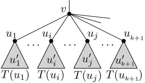
Before defining the types, we need to define the trace of a vertex in . To get some intuition, look at the rotation depicted in Figure 2. Note that, for each of the subtrees that are children of in , what determines whether they are children of or in the resulting subtree is whether some vertex in is adjacent to or not. Iterating this idea, if we are about to perform at most rotations starting from , then the behavior of such a subtree , assuming that no vertex of it is used by a rotation, is determined by its neighborhood in a set of ancestors of size at most the diameter of , and this is what the trace is intended to represent. That is, the trace of a vertex in , denoted by , captures “abstractly” the neighborhood of the whole subtree rooted at among (the ordered set of) its ancestors within the designated vertex set ; see 4.8 for the formal definition of trace and Figure 4 for an example. We stress that, when considering the neighborhood in the set of ancestors, we look at the whole subtree rooted at , and not only at its restriction to the set .
Equipped with the definition of trace, we can define the notion of type, which is somehow involved (cf. 4.9) and whose intuition behind is the following. For our marking algorithm to make sense, we want that if two vertices with the same parent (called -siblings) have the same type (within ), denoted by , and an -rotation sequence from to uses some vertex from but uses no vertex in , then there exists another -rotation sequence from to that uses vertices in instead of those in . To guarantee this replacement property, we need a stronger condition than just and having the same trace. Informally, we need them to have the same “variety of traces among their children within ”. More formally, this leads to a recursive definition where, in the leaves of (that are not necessarily leaves of ), the type corresponds to the trace, and for non-leaves, the type is defined by the trace and by the number of children of each possible lower type. Note that, a priori, the number of children of a given type may be unbounded, which would rule out the objective of bounding the number of types as a function of . To overcome this obstacle, the crucial and simple observation is that at most subtrees rooted at a vertex of contain vertices used by the desired rotation sequence (cf. 4.14). This implies that if there are at least -siblings of the same type, necessarily the whole subtree of at least one of them, say , will not be used by , implying that (and its whole subtree) achieves the desired parent in without being used by , and the same occurs to any other -sibling of the same type. Thus, keeping track of the existence of at least such children (regardless of their actual number) is enough to capture this “static” behavior, and allows us to shrink the possible distinct numbers to keep track of to a function of (cf. Equation 4, where the “” is justified by the previous discussion). Finally, for technical reasons we also incorporate into the type of a vertex its desired parent in , in case it defers from its parent in (cf. function ). See 4.9 for the formal definition of type and Figure 5 for an example with .
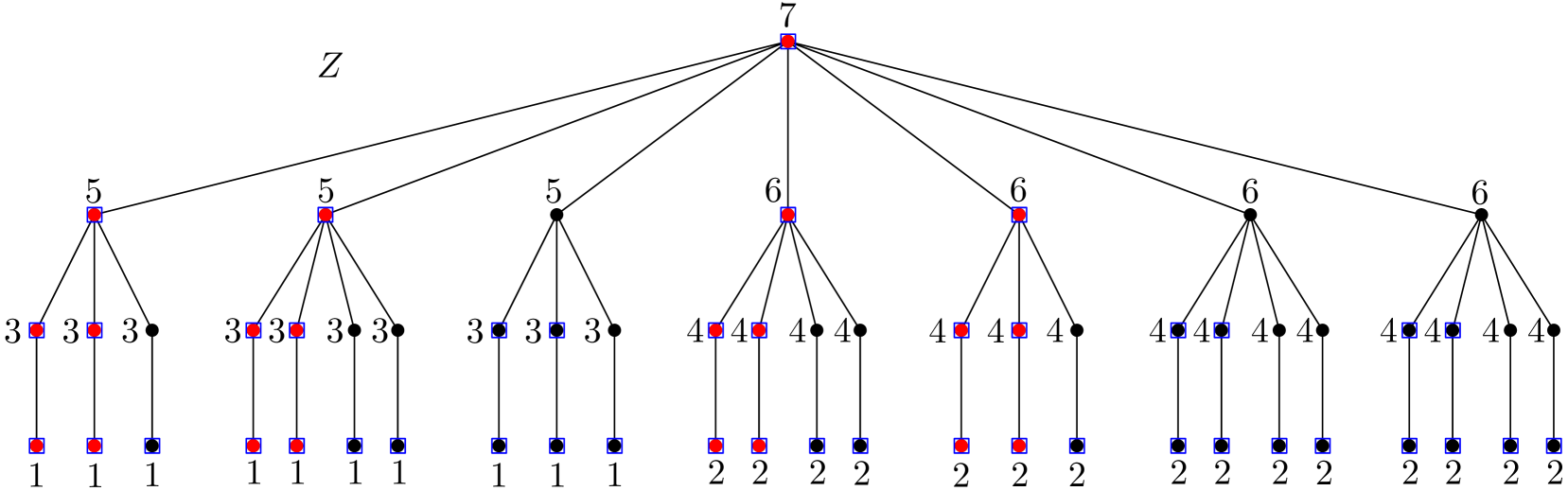
We prove (cf. 4.10) that the number of types is indeed bounded by a (large) function depending only on , and this function is what yields the upper bound on the asymptotic running time of the FPT algorithm of Theorem 1.1. Moreover, we show (cf. subsection 4.3) that the type of a vertex can be computed in time . We then use the notion of type and the bound given by 4.10 to define the desired set of size bounded by a function of . In order to find , we apply a marking algorithm on , that first identifies a set of pre-marked vertices, whose size is not necessarily bounded by a function of , and then “prunes” this set in a root-to-leaf fashion to find the desired set of marked vertices of appropriate size. See Figure 6 for an example of the marking algorithm for . We define (where denotes the set of connected components), and we call it the set of marked vertices of . We prove (cf. 4.12) that the size of is roughly equal to the number of types, and that the set can be computed in time FPT.
Once we have our set of marked vertices at hand, it remains to prove that we can restrict the rotations to use only vertices in . This is proved in our main technical result (cf. 4.16), whose proof critically exploits the recursive definition of the types. In a nutshell, we consider an -rotation sequence from to , for some , minimizing, among all -rotation sequences from to , the number of used vertices in . Our goal is to define another -rotation sequence from to using strictly less vertices in than , contradicting the choice of . To this end, let be a furthest (with respect to the distance to ) non-marked vertex of that is used by . We distinguish two cases.
In Case 1, we assume that has a marked -sibling with (cf. Figure 8). It is not difficult to prove that we can define from by just replacing with in all the rotations of involving (cf. 4 and 5).
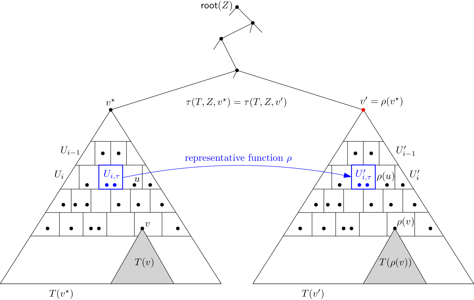
In Case 2, all -siblings of with , if any, are non-marked. In this case, in order to define another -rotation sequence from to that uses more marked vertices than , we need to modify in a more global way than in Case 1. Namely, in order to define , we need a more global (and involved) replacement, which we achieve via what we call a representative function . To define , we first guarantee the existence of a very helpful vertex that is a non-marked ancestor of having a marked -sibling of the same type such that no vertex in is used by ; see 6 and Figure 9. Exploiting the recursive definition of type, we then define our representative function , mapping vertices used by in to vertices in of the same type (cf. 7), and prove that we can define from by replacing each vertex used by in by its image via in in all the rotations of involving (cf. 8 and 9).
3 Preliminaries
Graphs.
We use standard graph-theoretic notation, and we refer the reader to [18] for any undefined terms. An edge between two vertices of a graph is denoted by . For a graph and a vertex set , the graph has vertex set and edge set . A connected component of a graph is a connected subgraph that is maximal (with respect to the addition of vertices or edges) with this property. We let denote the set of connected components of a graph . The distance between two vertices in , denoted by , is the length of a shortest path between and in . The diameter of , denoted by , is the maximum length of a shortest path between any two vertices of . We will often consider distances and the diameter of some rooted tree that is (a subtree of) an elimination tree of a graph . We stress that refers to the distance between and in , not in , and the same applies to .
For a graph , a vertex , and an integer , we denote by the set of vertices within distance at most from in , including itself. For a set , we let . For a subgraph of , we use as a shortcut for . In all these notations, we omit the superscript in the case where , that is, to refer to the usual neighborhood.
For a positive integer , we let denote the set . If is a function between two sets and and , we denote by the restriction of to .
Rooted trees.
For a rooted tree , we use to denote its root. For a vertex , we denote by the unique parent of in (or the empty set if is the root), by the set of children of in , by the set of ancestors of in (including itself), and by the set of descendants of in (including itself). The strict ancestors (resp. descendants) of are the vertices in the set (resp. ). We denote by the subtree of rooted at . Two vertices are -siblings if .
Rotation of an edge in an elimination tree.
We provide the formal definition of the rotation operation, which has been already informally defined in the introduction (cf. Figure 2).
Definition 3.1 (rotation operation).
Let be an elimination tree of a graph and let with . The rotation of in creates another elimination tree of defined as follows, where for better readability we use :
-
1.
.
-
2.
.
-
3.
If , let . Then .
-
4.
.
-
5.
Let . If is adjacent in to some vertex in , then ; otherwise .
-
6.
For every vertex , .
A -rotation sequence from an elimination tree to another elimination tree (of the same graph ) is an ordered set of edges such that, letting inductively and, for , with , we have that . In other words, a -rotation sequence consists of the ordered list of the edges to be rotated in order to obtain from , going through the intermediate elimination trees (of the same graph ). Clearly, if and only if there exists an -rotation sequence from to for some . We say that a vertex is used by a rotation sequence if it is an endpoint of some of the edges that are rotated by .
Parameterized complexity.
A parameterized problem is a language , for some finite alphabet . For an instance , the value is called the parameter. Such a problem is fixed-parameter tractable (FPT for short) if there is an algorithm that decides membership of an instance in time for some computable function . Consult [16, 33, 20, 19, 21] for background on parameterized complexity.
4 Formal description of the FPT algorithm
In this section we present our FPT algorithm to solve the Rotation Distance problem. We start in subsection 4.1 by providing some definitions and useful observations about the so-called good and bad vertices. In subsection 4.2 we show that we can assume that all the rotations involve vertices within balls of small radius around bad vertices. In subsection 4.3 we describe our marking algorithm, using the definition of type, and show that the set of marked vertices can be computed in FPT time. In subsection 4.4 we prove our main technical result (4.16), stating that we can restrict the desired rotations to involve only marked vertices. Finally, in subsection 4.5 we wrap up the previous results to prove Theorem 1.1.
4.1 Good and bad vertices
Throughout the paper, we assume that all the considered elimination trees are of a same fixed graph . For simplicity, we may assume henceforth that the considered input graph is connected.
Our algorithm exploits how a rotation in an elimination tree may affect the parents and the children of its vertices. Note that a single rotation of an edge , yielding an elimination tree , may change the parent of arbitrarily many vertices. Indeed, these vertices are the roots of the red subtrees in Figure 2, and the considered vertex may be adjacent to the root of arbitrarily many subtrees containing at least one vertex adjacent to : for each such root , but . As a concrete example, in Figure 1, but . On the other hand, item 6 of 3.1 implies that there are at most three vertices whose children set changes from to , namely as depicted in Figure 2. (Note that the sets of children of and always change, and that of changes provided that this vertex exists.) We state this observation formally, since it will be extensively used afterwards.
One rotation may change the set of children of at most three vertices.
The above discussion motivates the following definition.
Definition 4.1 (bad vertices).
Given two elimination trees and , a vertex is -children-bad (resp. (T,T’)-parent-bad) if (resp. ). A vertex is -bad if it is -children-bad, or -parent-bad, or both. A vertex is -good if it is not -bad.
Note that contains no -children-bad (or -parent-bad, or just -bad) vertices if and only if , that is, if and only if . Also, note that a vertex is -children-bad, with , if and only if at least one of its children is -parent-bad. subsection 4.1 directly implies the following necessary condition for the existence of a solution.
Given two elimination trees and , if then the number of -children-bad vertices is at most .
subsection 4.1 is equivalent to saying that we can safely conclude that any instance of Rotation Distance with at least -children-bad vertices is a no-instance. Thus, we can assume henceforth that we are dealing with an instance of Rotation Distance containing at most -children-bad vertices.
4.2 Restricting the rotations to small balls around bad vertices
Our next goal is to prove (4.3) that we can assume that the desired sequence of at most rotations to transform into uses only edges whose both endvertices lie in the union of all the balls of appropriate radius (depending only on ) around -children-bad vertices of , whose number is bounded by a function of by subsection 4.1.
In the next definition, for the sake of notational simplicity we omit , and from the notation , as we assume that they are already given, and fixed, as the input of our problem. We include in the considered set for technical reasons, namely in the proof of 2.
Definition 4.2 (union of balls of children-bad vertices).
Let be the set of -children-bad vertices. We define .
Lemma 4.3.
If , then there exists an -rotation sequence from to , with , using only vertices in .
Proof 4.4.
Let be an -rotation sequence from to , with . Let us denote by the number of edges in with at least one endvertex not in . Assuming that , we proceed to construct another -rotation sequence from to , with , such that . Repeating this procedure eventually yields a sequence as claimed in the statement of the lemma.
For , let be the -th edge of and let be the elimination tree obtained after the rotation of . Let also . For , we say that a vertex is affected by the rotation of if , and it is -affected if it is affected by the rotation of some edge in . Recall that a rotation affects at most three vertices, and that these vertices are within distance at most two in the original tree (cf. vertices in Figure 2). Moreover, any rotation may increase or decrease vertex distances by at most one, that is, for any and any two vertices , it holds that
| (1) |
Let be the set of -affected vertices, and note that . The observation above about the fact that the (two or three) vertices affected by a rotation are within distance at most two (in the tree where the rotation is done), together with Equation 1, imply that for every , it holds that
| (2) |
Since by assumption , there exists such that or (or both); assume without loss of generality that . Let be the connected component of containing vertices and (note that they indeed lie in the same component of since edge belongs to ). Let be the set of -children-bad vertices, and recall that . See Figure 3.
Claim 1.
No vertex in is -children-bad.
Proof 4.5 (Proof of claim).
Suppose towards a contradiction that the statement does not hold, and let . Since (see Figure 3), the definition of implies that , contradicting Equation 2 because both and belong to .
Claim 2.
All vertices in are -good.
Proof 4.6 (Proof of claim).
By 1, we only need to prove that no vertex in is -parent-bad. Since and no vertex in is -children-bad, the only vertex in that may be -parent-bad is its root, say . Vertex cannot be the root of , since in that case, the definition of and Equation 2 would imply that , a contradiction. Thus, since is not the root of , it has a parent in . But then, if were -parent-bad, then would be -children-bad, so , implying in turn that would also belong to the connected component of , contradicting the fact that .
Relying on 2, we define from an -rotation sequence from to , with , as follows: consists of the (ordered) edges appearing in , except from those with both endvertices lying in the connected component of .
Claim 3.
is an -rotation sequence from to with and .
Proof 4.7 (Proof of claim).
Note first that Equation 1 implies that both endpoints of any edge occurring in belong to the same connected component of , and therefore removing from those rotations with both endvertices in indeed results in a valid -rotation sequence from to another elimination tree of , in the sense that the edge rotations appearing in can indeed be done in a sequential way. Since at least edge has been removed from , it follows that (even if would be enough for our purposes) and that .
To conclude the proof, it just remains to verify that . We will do that by verifying that, for every vertex , it holds that and . We distinguish two cases.
Consider first a vertex . In this case, and its neighbors are involved in the same rotations in and in . Since is an -rotation sequence from to , we get that indeed and .
Finally, consider a vertex . By 2, is -good, implying that and . Since no rotation of involves , we get that and .
The above claim concludes the proof of the lemma.
By 4.3, we focus henceforth on trying to find an -rotation sequence from to , with , consisting only of edges with both endvertices in . First, we will consider each of the at most connected components of separately. In fact, we can get a better bound, as if has at least connected components, we can immediately conclude that we are dealing with a no-instance, since at least one rotation is needed in each component. Thus, we may assume that has at most connected components. On the other hand, since is defined as the union of at most balls of radius , it follows that every satisfies
| (3) |
Thus, by Equation 3, the “only” obstacle to obtain the desired FPT algorithm is that the vertices in can have an arbitrarily large degree. Note that in the particular case where the underlying graph has bounded degree, for instance if is a path [14, 25, 26, 28], the maximum degree of any elimination tree of is bounded, and therefore in that case is bounded by a function of , and an FPT algorithm follows immediately. To the best of our knowledge, this result was not known for graphs other than paths.
4.3 Description of the marking algorithm
As discussed in section 2, our strategy to deal with high-degree vertices in is as follows. For each connected component , our goal is to identify a subset of size bounded by a function of , such that we can restrict our search to rotations involving only pairs of vertices in . Clearly, this would yield the desired FPT algorithm. To find such a “small” set , we define the notion of type of a vertex , in such a way that the number of different types is bounded by a function of . Then, we will prove that it is enough to keep in , for each type, a number of vertices bounded again by a function of .
Let henceforth be a connected component of , which we consider as a rooted tree with its own set of leaves, which are not necessarily leaves in . We define to be the vertex in closest to in .
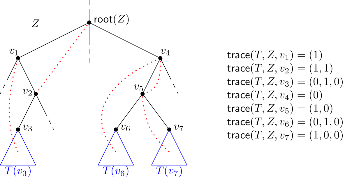
Before defining the types, we need to define the trace of a vertex in a designated vertex set that will correspond to a connected component of . Roughly speaking, the trace of a vertex captures “abstractly” the neighborhood of a (whole) subtree rooted at among (the ordered set of) its ancestors within the designated vertex set . We stress that, when considering the neighborhood in the set of ancestors, we look at the whole subtree rooted at , and not only at its restriction to the set .
Definition 4.8 (trace of a vertex in a component ).
Let be an elimination tree (of a graph ), let be a rooted subtree of corresponding to a connected component of , and let . The trace of in , denoted by , is a binary vector of dimension defined as follows (note that if , then its trace is empty). For , let be the ancestor of in such that . Then the -th coordinate of is if for some vertex , and otherwise.
See Figure 4 for an example of the trace of some vertices in a component .
For a vertex , let be equal to if , and to otherwise. Note that, by subsection 4.1, the function can take up to distinct values when ranging over all .
Definition 4.9 (type of a vertex in a component ).
Let be an elimination tree (of a graph ), let be a rooted subtree of corresponding to a connected component of , and let . The type of vertex , denoted by , is recursively defined as follows, where is the set of types occurring in the children of :
-
•
If is a leaf of , then consists of the pair .
-
•
Otherwise, consists of a tuple , where is a mapping defined such that, for every ,
(4)
See Figure 5 for an example for of how the types are computed in a component .
Lemma 4.10.
The set has size bounded by a function , with
| (5) |
Proof 4.11.
Let , and note that by Equation 3. For , let be the number of distinct types among the vertices in that are at distance exactly from in . Formally,
| (6) |
By the definition of type, since, on the one hand, all vertices at distance from are leaves of , and the number of possible traces among leaves is at most , and on the other hand the term corresponds to the possible distinct values of the function . For every , Equation 4 implies that
| (7) |
where the term again comes from the possible distinct values of the function , the term comes from the possible different traces within distance from , and the term follows from the fact that, for every , the function can take up to values for each type of a children of , together with the possibility that a type is not present among the children of . Note that a vertex with may have children being roots of any possible subtree with diameter at most , justifying the sum in Equation 7. Clearly, the upper bound of Equation 7 is maximized for , that is, for the children of , yielding the bound claimed in Equation 5.
Note that, in order to compute the type of a vertex in a component , the recursive definition of the types together with 4.10 easily imply the following observation, where the term comes from checking the neighborhood of within the set in the computation of the trace (cf. 4.8).
Let be an elimination tree of a graph , let be a rooted subtree of corresponding to a connected component of , and let . Then can be computed in time , where is the function from 4.10.
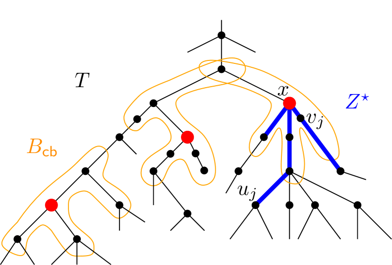
We will now use the notion of type and the bound given by 4.10 to define the desired set of size bounded by a function of . In order to find , we apply a marking algorithm on , that first identifies a set of pre-marked vertices, whose size is not necessarily bounded by a function of , and then “prunes” this set in a root-to-leaf fashion to find the desired set of marked vertices of appropriate size.
Start with . For every vertex and every , do the following:
-
•
If , add the whole set to .
-
•
Otherwise, add to an arbitrarily chosen subset of of size .
Finally, add to . We define and we call it the set of pre-marked vertices of .
We are now ready to define our bounded-size set . Start with and for , proceed inductively as follows: if is a vertex with that already belongs to , add to the set . Finally, for every -children-bad vertex of that belongs to , we add to the set . This concludes the construction of . Note that if a vertex belongs to , then the whole set belongs to as well. We define , and we call it the set of marked vertices of . See Figure 6 for an example of the marking algorithm.
Lemma 4.12.
The set of marked vertices has size bounded by a function , where has the same asymptotic growth as the function given by 4.10. Moreover, can be computed in time .
Proof 4.13.
Let us analyze the size of each set of separately, as their number is at most , and this factor gets subsumed by the asymptotic growth of . The diameter of is at most by Equation 3, so in order to bound the size of , it just remains to bound the degree of . By construction of , every vertex has at most children, where the term corresponds to the maximum number of -children-bad vertices (cf. subsection 4.1) that, together with their ancestors, have been marked within . Since the set is defined by pre-marking, for each vertex, at most children of each type, the set has size at most , where is the function given by 4.10. Thus, , where has the same asymptotic growth as .
As for computing the set in time , it follows from the definition of (that uses the set of pre-marked vertices ), that can be computed in time that is asymptotically dominated by computing the type of a vertex, which is bounded by by subsection 4.3.
4.4 Restricting the rotations to marked vertices
In this subsection we prove our main technical result (4.16), which immediately yields the desired FPT algorithm combined with 4.12 (whose proof uses 4.3), as discussed in subsection 4.5. We first need an easy lemma that will be extensively used in the proof of 4.16.
Lemma 4.14.
Let be an -rotation sequence from to , for some . For every vertex , there are at most vertices such that uses a vertex in each of the rooted subtrees .
Proof 4.15.
Assume towards a contradiction that there is a vertex having children, say , such that uses vertices with for . Then, since is made of at most rotations, by the pigeonhole principle necessarily there exist two children of and an integer such that , and none of occurs in any other rotation of other than . Since , it means that in the elimination tree where this rotation takes place, namely , it holds that . See Figure 7 for an illustration.
On the other hand, note that if is an elimination tree resulting from an elimination tree after the rotation of an edge , and are vertices of (and ) such that and , then necessarily , that is, necessarily the rotation involves at least one of and . See Figure 2 for a visualization of this claim, where the new edges that appear after the rotation of are and the edges between and some of the red subtrees: each of these new edges contains or .
Since because , and are -siblings, and , by the above paragraph there exists some integer , with , such that the rotation of contains at least one of and . This contradicts that fact that none of occurs in any other rotation of other than .
Note that, if in the statement of 4.14 we replaced “at most vertices” with “at most vertices”, then its proof would be trivial, as any of the at most rotations of involves two vertices, so at most distinct vertices overall. In that case, for the proof of 4.16 to go through, we would have to replace, in Equation 4 in the definition of type, “” with “” when taking the minimum. In the sequel we will often use a weaker version of 4.14, namely that for every vertex , at most vertices in are used by an -rotation sequence from to .
We are now ready to prove our main lemma.
Lemma 4.16.
If , then there exists an -rotation sequence from to , with , using only vertices in .
Proof 4.17.
Let be an -rotation sequence from to , for some , minimizing, among all -rotation sequences from to , the number of vertices in (that is, the non-marked vertices) used by . Note that exists by the hypothesis that . If there are no vertices in used by , then we are done, so assume that there are. Our goal is to define another -rotation sequence from to using strictly less vertices in than , contradicting the choice of and concluding the proof.
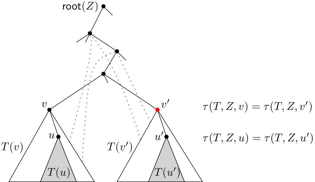
To this end, let be a furthest (with respect to the distance to ) non-marked vertex of that is used by . By 4.3, we can assume that . Let be the connected component of such that . For technical reasons, it will be helpful to assume that is not a leaf of . (This can be achieved, for instance, by observing that the analysis of the size of the components in 4.3 is not tight. Alternatively, we can just “artificially” increase their diameter by one –i.e., replacing with in the definition of – so that we can safely assume that the leaves of are never used by a rotation sequence.) Note that the choice of as a lowest (i.e., furthest) non-marked vertex of used by implies that for every vertex , the whole subtree remains intact throughout , meaning that it appears as a rooted subtree in all the intermediate elimination trees generated by the -rotation sequence . We distinguish two cases, the second one being considerably more involved, but that will benefit from the intuition developed in the first one.
Case 1: has a marked -sibling with .
Since is non-marked and by assumption it has some marked -sibling, the definition of (namely, that up to vertices of each type are recursively marked) and 4.14 imply that has some marked -sibling of the same type that is not used by . Let without loss of generality be such a -sibling of . Note that the choice of as a lowest non-marked vertex used by implies that the whole subtree remains intact throughout . See Figure 8 for an illustration. In this case, we define from by just replacing with in all the rotations of involving . We need to prove that is well-defined (that is, that the edges to be rotated do exist in the intermediate elimination trees) and that it is an -rotation sequence from to . Once this is proved, this case is done, as uses strictly more marked vertices than .
Claim 4.
is a well-defined -rotation sequence.
Proof 4.18 (Proof of claim).
We need to prove that if and for some and some , then . Let us prove it by induction. For , assume that for some . The choice of as a lowest non-marked vertex of used by implies that , and since is a -sibling of , it follows that . Assume now inductively that the edges to be rotated exist up to , and suppose that for some . Since , it follows in particular that (see the green dotted edges in Figure 8), and as and are -siblings, it follows that the rooted subtrees and have exactly the same neighbors in the set , that is,
| (8) |
Equation 8 implies that, up to , vertex has been following exactly the same moves in as the ones followed by vertex in . Thus, the fact that implies that , and the claim follows.
Claim 5.
is an -rotation sequence from to .
Proof 4.19 (Proof of claim).
By 4, is an -rotation sequence from to some elimination tree of . It remains to prove that . This is equivalent to proving that, for every vertex that is not a root in or , . By definition of , this is clearly the case for every vertex that is not in the set .
Consider first a vertex . Note that the whole rooted subtree remains intact throughout , in the same way as remains intact throughout . Moreover, since all -children-bad vertices belong to , and does not, it follows that is not -children-bad, that is, that . This implies that for every vertex .
Consider now vertices and . The choice of as a lowest non-marked vertex used by implies that all the descendants of in are -good, except maybe itself that may be -parent-bad. If that is the case, the hypothesis that and the fact that the function is part of the definition of the type of a vertex imply that is also -parent-bad and that . Recall that Equation 8 discussed above implies that follows in the same moves that follows in . And since , including the case where both sets are empty, it follows that .
Finally, consider a vertex . Note that the whole subtree remains intact throughout , in the same way as the whole subtree remains intact throughout for every vertex . Since such a vertex is -good by the choice of , we have that . The fact that implies, similarly to the discussion after Equation 8, that the subtree follows in the same moves followed by in , where is a vertex such that , which exists by the recursive definition of type (cf. 4.9) and the hypothesis that ; see Figure 8. Thus, , and the claim follows.
Case 2: all -siblings of with , if any, are non-marked.
In this case, in order to define another -rotation sequence from to that uses more marked vertices than , we need to modify in a more global way than what we did in Case 1 above, where it was enough to replace vertex with a marked -sibling of the same type. Now, in order to define , we need a more global replacement. To this end, the following claim guarantees the existence of a very helpful vertex . See Figure 9 for an illustration.
Claim 6.
There exists a unique vertex such that
-
•
is non-marked,
-
•
has a marked -sibling such that
-
–
, and
-
–
no vertex in is used by , and
-
–
-
•
is the vertex closest to satisfying the above properties.
Proof 4.20 (Proof of claim).
Since and , the definition of the marking algorithm implies that there exists a marked -sibling of with . Moreover, the fact that is defined by recursively marking up to vertices of each type implies, together with 4.14 and the fact that the desired vertex is non-marked, that there is some -sibling of with such that no vertex in is used by . Finally, we can clearly choose in a unique way as being the vertex closest to satisfying the above properties.
Note that Case 1 of the proof corresponds to the particular case where is equal to itself, but we prefer to separate both cases for the sake of readability. Intuitively, we will apply recursively the argument of Case 1 to the rooted subtrees and , starting with and , exploiting the definition of types to appropriately define the desired replacement of vertices to construct from .
Formally, let be the set of vertices in used by (so in Case 1, ), and let be the injective function defined as follows. For , let be the set of vertices in used by that are at distance exactly from vertex in . Note that some of the sets may be empty, and that contains . For every type occurring in a vertex in , let be the set of vertices of type in . Note that, if a set is non-empty, then defines a partition of into non-empty sets. Let be a set of marked vertices of type in of size (we shall prove in 7 that it exists). Then we define as any bijection between and . See Figure 9 for an illustration.
Claim 7.
The function is well-defined and injective.
Proof 4.21 (Proof of claim).
Assuming that the sets exist, it is clear that is injective. Hence, we shall prove that for every and every type occurring in a vertex in , there exists a set of marked vertices of type with . We proceed by induction on . For , and the only type occurring in is . Thus, we can just take , where is the vertex given by 6, so that . We now prove the statement for any , using the recursive definition of type (cf. 4.9). We may assume that , as otherwise there is nothing to prove. The facts that and that is marked imply that, for every and every type , the following holds:
-
•
If contains a set of at most vertices of type , all at distance exactly from , then contains a set of marked vertices of type with , all at distance exactly from .
-
•
If contains a set of at least vertices of type , all at distance exactly from , then contains a set of marked vertices of type with , all at distance exactly from .
It is important to pay attention to the difference between the above two items: while in the first one the set of marked vertices has the same size as , in the second one we can “only” guarantee, due to Equation 4, that , even if may be arbitrarily larger (even of size not bounded by any function of ). Fortunately, thanks to 4.14, this is enough for finding the desired set in order to define the representative function , as we proceed to discuss. Note that, for every and every type , it holds that , since may use only some of the vertices in .
Suppose first that, for some and some type , the first item above holds. Then, since , we can just take as any subset of of size .
Suppose now that the second item above holds, that is, that contains a set of at least vertices of type , all at distance exactly from . By 4.14, it holds that , and since , we can indeed define as any subset of of size , and the claim follows.
For every vertex (recall that is the set of vertices in used by ), the vertex is called the representative of . Note that the function is also defined on , since it is used by . We now define from by replacing, in the rotations defining the sequence, every vertex by its representative .
The following two claims correspond respectively to 4 and 5 of Case 1, and conclude the proof of the lemma.
Claim 8.
is a well-defined -rotation sequence.
Proof 4.22 (Proof of claim).
Similarly to the proof of 4, we need to prove that if , then for every the corresponding edge to be rotated in exists in the intermediate subtree. Suppose that is a rotation in , for some , such that for some . We distinguish three cases depending to whether the vertices involved in the rotation belong to or not.
-
•
Suppose first that none of belongs to . It is not difficult to verify that if , then as well, where is the tree obtained from by applying the first rotations of . Indeed, the fact that implies that the existence of such an edge with both endpoints outside is preserved when replacing the vertices in with their representatives.
-
•
Suppose now that both belong to . In this case, the edge of has been replaced by in . Note that both vertices belong to . The definition of the representative function implies that and , which in particular implies that and . It follows that vertex (resp. ) has been following the same moves within in as the ones followed by vertex (resp. ) within in . Thus, the fact that implies that .
-
•
Finally, suppose without loss of generality that and . This case is similar to the proof of 4, with the role of replaced with . Namely, it can be proved by induction on in a similar fashion. For , assume that with and . Then, by the definition of (cf. 6), necessarily and . Since and is a -sibling of , it follows that .
Assume now inductively that the edges to be rotated exist up to , and suppose that for some and . The fact that implies that , which implies in particular that and have exactly the same neighbors in the set , that is,
(9) The fact that and Equation 9 imply that, up to , vertex has been following the same moves within and in as the ones followed by vertex within and in . Thus, the fact that implies that , and the claim follows.
Claim 9.
is an -rotation sequence from to .
Proof 4.23 (Proof of claim).
The proof of this claim follows that of 5. By 8, is an -rotation sequence from to some elimination tree of . It remains to prove that . This is equivalent to proving that, for every vertex that is not a root in or , . By definition of , this is clearly the case for every vertex that is not in the set , given that . We distinguish three cases to deal with the vertices in .
-
•
Consider first a vertex different from . Note that the whole rooted subtree remains intact throughout , in the same way as the whole subtree remains intact throughout . Moreover, since all -children-bad vertices belong to , and does not (cf. 6), it follows that is not -children-bad, that is, that for every vertex . This implies that for every vertex different from .
-
•
Consider now vertices and . The definition of (cf. 6) implies that all the descendants of in are -good, except maybe itself that may be -parent-bad. If that is the case, the fact that and the fact that the function is part of the definition of the type of a vertex imply that is also -parent-bad and that . Similarly to Equation 8, the fact that implies that
(10) which implies that follows in the same moves that follows in . And since , including the case where both sets are empty, it follows that .
-
•
Finally, consider a vertex different from . First note that if neither nor any descendant of in (including itself) are used by , then, since no vertex in is used by , it follows that .
We now proceed recursively, by first considering a lowest vertex such that is used by . Note that such a vertex exists because (at least) is used by and we may assume that the leaves of are not used by , so by definition of this is also the case for the leaves of . Note that, by the choice of , the whole subtree remains intact throughout . Since such a vertex is -good because no vertex in is used by , we have that . The fact that implies that the subtree follows in the same moves within as the moved followed by in within , where is a vertex such that , which exists by the recursive definition of type and the hypothesis that . Thus, .
Finally, we consider vertices bottom-up in , assuming inductively that their strict descendants in already have their desired parent in and exploiting the recursive definition of type. When encountering such a vertex , we further distinguish three cases.
-
–
If neither nor are used by , since no vertex in is used by , it follows that .
-
–
If is used by , the analysis is similar to the case of in the proof of 5 (cf. Figure 8), by replacing the roles of and in 5, respectively, by and , where is a vertex such that . Note that is used by and that . We can recursively assume that for all strict descendants of , . The fact that implies that follows in within the same moves that follows in within . And since (recall that the function is part of the definition of type), including the case where both sets are empty (meaning that they already have their respective desired parents), and since the whole subtree remained intact throughout , it follows that .
-
–
Otherwise, if is not used by but is used by , we apply the same arguments as in the case where is a lowest such a vertex as discussed above, by replacing the property that “the whole subtree remains intact throughout ” with “for every strict descendant of , it holds that ”, which we can recursively assume. Thus, we conclude in the same way that .
-
–
The proof of the claim is now complete.
By 9, is an -rotation sequence from to , and it uses strictly more marked vertices than , because no vertex of is marked (by the conditions in 6), and within there is at least one marked vertex, namely . This concludes Case 2.
In both cases, we have defined from another -rotation sequence from to using strictly less vertices in than , contradicting the choice of and concluding the proof of the lemma.
4.5 Wrapping up the algorithm
We finally have all the ingredients to prove our main result, which we restate for convenience.
See 1.1
Proof 4.24.
Given a connected graph , two elimination trees and of , and a positive integer as input of the Rotation Distance problem, we proceed as follows.
By subsection 4.1, we can assume that our instance contains at most -children-bad vertices, which can be clearly identified in time linear in . Recall from 4.2 that, if we let be the set of -children-bad vertices, . By 4.3, If , then there exists an -rotation sequence from to , for some , using only vertices in .
We now apply our marking algorithm to find the set of marked vertices. By 4.12, the set has size at most and can be computed in time , where has the same asymptotic growth as the function given by 4.10. By 4.16, if , then there exists an -rotation sequence from to , for some , using only vertices in .
Thus, we can solve the problem by applying the following naive brute force algorithm: for every (we may assume that and are distinct), we guess all possible sets of ordered pairs of vertices in (so, vertices overall, allowing repetitions), and for each such an ordered set of pairs, we apply the corresponding rotations to and check whether the resulting elimination tree is equal to or not, which can be done in time linear in . Naturally, if for some of the guessed pairs to be rotated, that edge does not exist in the corresponding intermediate elimination tree of , we discard that guess.
The running time of the resulting algorithm is upper-bounded by , and the theorem follows.
5 Further research
We proved that the Rotation Distance problem, for a general graph , can be solved in time , where is the function given by Theorem 1.1. This function is quite large, and it is worth trying to improve it. The growth of is mainly driven by the number of different types of vertices (cf. 4.9) that we consider in our marking algorithm. We need this recursive definition of type to guarantee that, when two vertices have the same type, then for each possible type and every integer at most the bound given in Equation 3, vertices and have the same number (up to ) of descendants of type within distance . This is exploited, for instance, in Case 2 of the proof of 4.16 to apply a recursive argument. It may possible to find a simpler argument in the replacement operation performed in the proof of 4.16 (using the representative function , and in that case, one may allow for a less refined notion of type, leading to a better bound.
Another natural direction is to investigate whether Rotation Distance admits a polynomial kernel parameterized by . So far, this is only known when the considered graph is a path, where even linear kernels are known[14, 30]; see Table 1. As an intermediate step, one may consider graphs of bounded degree, for which it seems plausible that 4.3 (restriction to few balls of bounded diameter) provides a helpful opening step.
Finally, Ito et al. [24] also proved the NP-hardness of a related problem called Combinatorial Shortest Path on Polymatroids, relying on the fact that graph associahedra can be realized as the base polytopes of some polymatroids [35]. To the best of our knowledge, the parameterized complexity of this problem has not been investigated.
References
- [1] Georgy M. Adel’son-Vel’skii and Evgenii M. Landis. An algorithm for the organization of information. Soviet Mathematics Doklady, 3:1259–1263, 1962. URL: https://zhjwpku.com/assets/pdf/AED2-10-avl-paper.pdf.
- [2] Oswin Aichholzer, Wolfgang Mulzer, and Alexander Pilz. Flip Distance Between Triangulations of a Simple Polygon is NP-Complete. Discrete & Computational Geometry, 54(2):368–389, 2015. doi:10.1007/S00454-015-9709-7.
- [3] Benjamin Aram Berendsohn. The diameter of caterpillar associahedra. In Proc. of the 18th Scandinavian Symposium and Workshops on Algorithm Theory (SWAT), volume 227 of LIPIcs, pages 14:1–14:12, 2022. doi:10.4230/LIPICS.SWAT.2022.14.
- [4] Nicolas Bousquet, Amer E. Mouawad, Naomi Nishimura, and Sebastian Siebertz. A survey on the parameterized complexity of reconfiguration problems. Computer Science Review, 53:100663, 2024. doi:10.1016/J.COSREV.2024.100663.
- [5] Jean Cardinal, Linda Kleist, Boris Klemz, Anna Lubiw, Torsten Mütze, Alexander Neuhaus, and Lionel Pournin. Working grup 4.2: Rotation distance between elimination trees. Report from Dagstuhl Seminar 22062: Computation and Reconfiguration in Low-Dimensional Topological Spaces, page 35. URL: https://drops.dagstuhl.de/storage/04dagstuhl-reports/volume12/issue02/22062/DagRep.12.2.17/DagRep.12.2.17.pdf.
- [6] Jean Cardinal, Stefan Langerman, and Pablo Pérez-Lantero. On the diameter of tree associahedra. Electronic Journal of Combinatorics, 25(4):4, 2018. doi:10.37236/7762.
- [7] Jean Cardinal, Arturo Merino, and Torsten Mütze. Efficient generation of elimination trees and graph associahedra. In Proc. of the 33rd ACM-SIAM Symposium on Discrete Algorithms (SODA), pages 2128–2140, 2022. doi:10.1137/1.9781611977073.84.
- [8] Jean Cardinal, Lionel Pournin, and Mario Valencia-Pabon. Diameter estimates for graph associahedra. Annals of Combinatorics, 26:873–902, 2022. doi:10.1007/s00026-022-00598-z.
- [9] Jean Cardinal, Lionel Pournin, and Mario Valencia-Pabon. The rotation distance of brooms. European Journal of Combinatorics, 118:103877, 2024. doi:10.1016/J.EJC.2023.103877.
- [10] Jean Cardinal and Raphael Steiner. Shortest paths on polymatroids and hypergraphic polytopes. CoRR, abs/2311.00779, 2023. arXiv:2311.00779.
- [11] Michael Carr and Satyan L. Devadoss. Coxeter complexes and graph-associahedra. Topology and its Applications, 153(12):2155–2168, 2006. doi:10.1016/j.topol.2005.08.010.
- [12] Cesar Ceballos, Francisco Santos, and Günter M. Ziegler. Many non-equivalent realizations of the associahedron. Combinatorica, 35(5):513–551, 2015. doi:10.1007/s00493-014-2959-9.
- [13] Sean Cleary. Restricted rotation distance between -ary trees. Journal of Graph Algorithms and Applications, 27(1):19–33, 2023. doi:10.7155/JGAA.00611.
- [14] Sean Cleary and Katherine St. John. Rotation distance is fixed-parameter tractable. Information Processing Letters, 109(16):918–922, 2009. doi:10.1016/J.IPL.2009.04.023.
- [15] Sean Cleary and Katherine St. John. A linear-time approximation algorithm for rotation distance. Journal of Graph Algorithms and Applications, 14(2):385–390, 2010. doi:10.7155/JGAA.00212.
- [16] Marek Cygan, Fedor V. Fomin, Lukasz Kowalik, Daniel Lokshtanov, Dániel Marx, Marcin Pilipczuk, Michal Pilipczuk, and Saket Saurabh. Parameterized Algorithms. Springer, 2015. doi:10.1007/978-3-319-21275-3.
- [17] Satyan L. Devadoss. A realization of graph associahedra. Discrete Mathematics, 309(1):271–276, 2009. doi:10.1016/J.DISC.2007.12.092.
- [18] Reinhard Diestel. Graph Theory. Springer-Verlag, Heidelberg, 5th edition, 2016. URL: https://link.springer.com/book/10.1007/978-3-662-53622-3.
- [19] Rod G. Downey and Michael R. Fellows. Fundamentals of Parameterized Complexity. Texts in Computer Science. Springer, 2013.
- [20] Jörg Flum and Martin Grohe. Parameterized Complexity Theory. Springer-Verlag, 2006. doi:10.1007/3-540-29953-X.
- [21] Fedor V. Fomin, Daniel Lokshtanov, Saket Saurabh, and Meirav Zehavi. Kernelization: Theory of Parameterized Preprocessing. Cambridge University Press, 2019. doi:10.1017/9781107415157.
- [22] Leonidas J. Guibas and Robert Sedgewick. A dichromatic framework for balanced trees. In Proc. of the 19th Annual Symposium on Foundations of Computer Science (FOCS), pages 8–21, 1978. doi:10.1109/SFCS.1978.3.
- [23] Christophe Hohlweg and Carsten E. M. C. Lange. Realizations of the associahedron and cyclohedron. Discrete & Computational Geometry, 37(4):517–543, 2007. doi:10.1007/S00454-007-1319-6.
- [24] Takehiro Ito, Naonori Kakimura, Naoyuki Kamiyama, Yusuke Kobayashi, Shun-ichi Maezawa, Yuta Nozaki, and Yoshio Okamoto. Hardness of Finding Combinatorial Shortest Paths on Graph Associahedra. In Prof. of the 50th International Colloquium on Automata, Languages, and Programming (ICALP), volume 261 of LIPIcs, pages 82:1–82:17, 2023. doi:10.4230/LIPIcs.ICALP.2023.82.
- [25] Iyad Kanj, Eric Sedgwick, and Ge Xia. Computing the flip distance between triangulations. Discrete & Computational Geometry, 58(2):313–344, 2017. doi:10.1007/S00454-017-9867-X.
- [26] Haohong Li and Ge Xia. An time FPT algorithm for convex flip distance. In Proc. of the 40th International Symposium on Theoretical Aspects of Computer Science (STACS), volume 254 of LIPIcs, pages 44:1–44:14, 2023. doi:10.4230/LIPICS.STACS.2023.44.
- [27] Jean-Louis Loday. Realization of the Stasheff polytope. Archiv der Mathematik, 83:267–278, 2004. doi:10.1007/s00013-004-1026-y.
- [28] Anna Lubiw and Vinayak Pathak. Flip distance between two triangulations of a point set is NP-complete. Computational Geometry, 49:17–23, 2015. doi:10.1016/J.COMGEO.2014.11.001.
- [29] Anna Lubiw and Vinayak Pathak. Flip distance between two triangulations of a point set is NP-complete. Computational Geometry, 49:17–23, 2015. doi:10.1016/J.COMGEO.2014.11.001.
- [30] Joan M. Lucas. An improved kernel size for rotation distance in binary trees. Information Processing Letters, 110(12-13):481–484, 2010. doi:10.1016/J.IPL.2010.04.022.
- [31] Thibault Manneville and Vincent Pilaud. Graph properties of graph associahedra. CoRR, abs/1409.8114, 2010. arXiv:1409.8114.
- [32] Jaroslav Nesetril and Patrice Ossona de Mendez. Sparsity - Graphs, Structures, and Algorithms, volume 28 of Algorithms and combinatorics. Springer, 2012. doi:10.1007/978-3-642-27875-4.
- [33] Rolf Niedermeier. Invitation to Fixed-Parameter Algorithms. Oxford University Press, 2006. doi:10.1093/acprof:oso/9780198566076.001.0001.
- [34] Alexander Pilz. Flip distance between triangulations of a planar point set is APX-hard. Computational Geometry, 47(5):589–604, 2014. doi:10.1016/J.COMGEO.2014.01.001.
- [35] Alex Postnikov, Victor Reiner, and Lauren Williams. Faces of generalized permutohedra. Documenta Mathematica, 13:207–273, 2008. doi:10.4171/DM/248.
- [36] Alexander Postnikov. Permutohedra, associahedra, and beyond. International Mathematics Research Notices, 2009(6):1026–1106, 2009. doi:10.1093/imrn/rnn153.
- [37] Lionel Pournin. The diameter of associahedra. Advances in Mathematics, 259:13–42, 2014. doi:10.1016/j.aim.2014.02.035.
- [38] Lionel Pournin. The asymptotic diameter of cyclohedra. Israel Journal of Mathematics, 219(2):609–635, 2017. doi:10.1007/s11856-017-1492-0.
- [39] Daniel D. Sleator, Robert E. Tarjan, and William P. Thurston. Rotation distance, triangulations, and hyperbolic geometry. Journal of the American Mathematical Society, 1(3):647–681, 1988. doi:10.1090/S0894-0347-1988-0928904-4.
- [40] Daniel Dominic Sleator and Robert Endre Tarjan. Self-adjusting binary search trees. Journal of the ACM, 32(3):652–686, 1985. doi:10.1145/3828.3835.
- [41] Richard P. Stanley. Catalan numbers. Cambridge University Press, 2015. doi:10.1017/CBO9781139871495.