The possible frustrated superconductivity in the kagome superconductors

Abstract

Geometric frustration has long been a subject of enduring interest in condensed matter physics. While geometric frustration traditionally focuses on magnetic systems, little attention is paid to the ”frustrated superconductivity” which could arise when the superconducting interaction conflicts with the crystal symmetry. The recently discovered kagome superconductors provide a particular opportunity for studying this due to the fact that the frustrated lattice structure and the interference effect between the three sublattices can facilitate the frustrated superconducting interaction. Here, we propose a theory that supports the frustrated superconducting state, derived from the on-site $s$-wave superconducting pairing in conjunction with the nearest-neighbor pairings hoping and the unique geometrical frustrated lattice structure. In this state, whereas the mutual $2\pi/3$ difference of the superconducting pairing phase causes the six-fold modulation of the amplitude and breaks the time-reversal symmetry with $4\pi$ phase changes of the superconducting pairing as one following it around the Fermi surface, it is immune to the impurities without the impurity-induced in-gap states and produces the pronounced Hebel-Slichter peak of the nuclear spin-lattice relaxation rate below $T_{c}$. Notably, the theory also reveals a disorder-induced superconducting pairing transition from the frustrated superconducting state to an isotropic $s$-wave superconducting state without traversing the nodal points, recovering and explaining the behavior found in experiment. This study not only serves as a promising proposal to mediate the divergent or seemingly contradictory experimental outcomes regarding superconducting pairing symmetry, but may also pave the way for advancing investigations into the frustrated superconducting state.

I Introduction

The discovery of superconductivity in a family of compounds AV₃Sb₅ (A=K, Rb, Cs), which share a common lattice structure with kagome net of vanadium atoms, has set off a new boom of researches on the superconductivity as well as the associated exotic quantum states  Ortiz1 ; SYYang1 ; Ortiz2 ; QYin1 ; KYChen1 ; YWang1 ; ZZhang1 ; YXJiang1 ; FHYu1 ; XChen1 ; HZhao1 ; HChen1 ; HSXu1 ; Liang1 ; CMu1 ; CCZhao1 ; SNi1 ; WDuan1 ; Xiang1 ; PhysRevX.11.041030 ; PhysRevB.104.L041101 ; ZLiu1 ; NatPhys.M.Kang ; YFu1 ; HTan1 ; Shumiya1 ; FHYu2 ; LYin1 ; Nakayama2 ; KJiang1 ; LNie1 ; HLuo1 ; Neupert1 ; YSong1 ; Nakayama1 ; HLi1 ; CGuo1 ; HLi2 ; HLi3 ; XWu1 ; Denner1 ; SCho1 ; YPLin3 ; LZheng1 ; CWen1 ; Tazai1 ; Jiang1 ; Mielke1 . The appealing aspects of these compounds lie in that they incorporate many remarkable properties of the electron structure, such as VHF, FS nesting and nontrivial band topology Ortiz1 . Meanwhile, the superconducting (SC) phase emerges next to a charge density wave phase in the pressure-temperature phase diagram. As the electrons in these materials suffer simultaneously from the geometrical frustration, topological band structure and the competition between different possible ground states, the observations of the superconductivity in these topological metals are in themselves exotic and rare. The connection to the underlying lattice geometry and the topological nature of the band structure further place them in the context of wider research efforts in topological physics and superconductivity.

To understand the underlying mechanism of the superconductivity in this family of kagome superconductors, the determination of the pairing symmetry of the SC order parameter is thought to be a prerequisite step. For this goal, numerous experiments with various means have been conducted in the past several years. However, inconsistent results were found so far in experimental measurements and data analysis, and some unusual features were discovered as well in the SC state of AV₃Sb₅. On the one hand, the SC pairings in these compounds are suggested to be of the conventional $s$-wave type, supported by the appearance of the Hebel-Slichter coherence peak just below $T_{c}$ in the nuclear magnetic resonance spectroscopy CMu1 and the nodeless SC gap in both the penetration depth measurements WDuan1 and the angle-resolved photoemission spectroscopy (ARPES) experiment YZhong1 . Intriguingly, recent magnetic penetration depth measurements also revealed a impurity induced transition from an anisotropic fully-gapped state to an isotropic full-gap state without passing through a nodal state Roppongi1 . On the other hand, the indications of time-reversal symmetry breaking discovered in the SC state Mielke1 ; YWang1 ; YWu1 , together with the nodal SC gap feature detected by some experiments HZhao1 ; CCZhao1 ; HSXu1 ; Liang1 ; HChen1 , hint to an unconventional superconductivity.

Although the majority of experimental evidence in the AV₃Sb₅ materials indicates that the superconductivity has a conventional origin with spin singlet $s$-wave pairing CMu1 ; WDuan1 ; YZhong1 ; YXie1 , the field is haunted by the seemingly divergent experimental observations regarding the pairing symmetry. Theoretically, a variety of possible pairing symmetries have been put forward in the kagome systems SLYu1 ; WSWang1 , ranging from the $s$-wave WSWang1 ; THan1 ; Tazai1 , $d$-wave, and extended $s_{ext}$-wave to $d_{x^{2}-y^{2}}+id_{xy}$-wave pairing symmetries SLYu1 ; WSWang1 ; Kiesel3 , and even triplet $p$-wave Tazai1 and $f$-wave pairing symmetries SLYu1 ; CWen1 ; XWu1 ; TZhou1 . Considering the interplay of the superconductivity and CDW phase, theoretical analysis has also shown that a conventional fully gapped superconductivity is unable to open a gap on the domains of the chiral $2\times 2$ charge density wave (CDW) and results in the gapless edge modes in the SC state YGu1 . A more direct consideration of the interplay between the superconductivity and the chiral $2\times 2$ CDW has revealed that a modulated and even nodal SC gap features show up albeit an on-site $s$-wave SC order parameter being included in the study HMJiang2 ; HMJiang3 ; TZhou2 . In this scenario, the coexistence of the conventional superconductivity and the chiral CDW has also been proposed to explain time-reversal symmetry breaking in the kagome superconductors HMJiang2 ; HMJiang3 ; TZhou1 .

Nevertheless, more recent experiments have evidenced that the time-reversal symmetry breaking has a direct connection to the SC state YWang1 ; TLe1 , especially in the case where the CDW order was fully suppressed by Ta atoms doping into CsV₃Sb₅ HDeng1 . While a variety of possible pairing states with time-reversal symmetry breaking have been proposed, there is still limited knowledge as to how the SC pairings that possess the conventional origin could have the intrinsic time-reversal symmetry breaking SC state.

In this paper, we propose a theory in which the conventional on-site $s$-wave SC pairing transforms to the time-reversal symmetry breaking SC state, as a result of the nearest-neighbor pairings hoping and the unique geometrical frustrated lattice structure. In this state, the phase of the SC pairing on the three sublattices mutually differs by $2\pi/3$, an analogy to the frustrated magnetism, which is dubbed as ”frustrated SC state” thereafter. The amplitude of the frustrated SC state modulates along the Fermi surface six-fold symmetrically without passing through the nodes. The frustrated SC state breaks the time-reversal symmetry explicitly with the $4\pi$ phase changes of the SC pairing as one following it around the Fermi surface, i.e., winding number of $2$. Though the frustrated SC state has the structure along the Fermi surface exactly as the $d_{x^{2}-y^{2}}+id_{xy}$-wave pairing, it is immune from the impurities without the impurity-induced in-gap states and produces the pronounced typical Hebel-Slichter peak of the nuclear spin-lattice relaxation rate below $T_{c}$. Particularly, the theory also reveals a disorder-induced SC pairing transition from the frustrated SC state to an isotropic $s$-wave SC state without passing through the nodal point, recovering the behavior found in experiment. This study not only serves as a promising proposal to mediate the divergent or seemingly contradictory experimental outcomes regarding SC pairing symmetry, but may also paves the way for further studies on the frustrated SC state.

The remainder of the paper is organized as follows. In Sec. II, we introduce the model Hamiltonian and carry out analytical calculations. In Sec. III, we present numerical calculations and discuss the results. In Sec. IV, we make a conclusion.

II model and method

Considering the SC pairing hoppings among the nearest-neighbor sites, the Hamiltonian of the system is modified by adding a pairing hopping term,

$$H_{PH} = J\sum_{\langle ij\rangle}(c^{{\dagger}}_{i\uparrow}c^{{\dagger}}_{i\downarrow}c_{j\downarrow}c_{j\uparrow}+h.c.)$$ (1)

where $c^{{\dagger}}_{i\sigma}$ creates an electron with spin $\sigma$ on the site $i$ of the kagome lattice and $\langle ij\rangle$ denotes nearest-neighbors (NN). Mimicking the NN magnetic interactions, we may define the SC operators $\tilde{\Delta}^{{\dagger}}_{i}\equiv c^{{\dagger}}_{i\downarrow}c^{{\dagger}}_{i\uparrow}$ and $\tilde{\Delta}_{j}\equiv c_{j\uparrow}c_{j\downarrow}$. Then, the pairing hopping term can be rewritten as,

$$H_{PH} = J\sum_{\langle ij\rangle}(\tilde{\Delta}^{{\dagger}}_{i}\tilde{\Delta}_{j}+H.c.).$$ (2)

On the geometry frustrated kagome lattice with positive pairing hopping $J$, the pairings on the three sublattices with the mutual phase differences $2\pi/3$ result in a maximal energy gain $-3J|\Delta|^{2}$, where we assume the pairing amplitudes on the three sublattice sites being the same. By comparison, while the energy gain is $-2J|\Delta|^{2}$ for the pairings on the three sublattices with one of them possessing the opposite phase, there is energy lost $6J|\Delta|^{2}$ for the pairings with identical phase. Thus, we are encountered with the SC version of the spin frustration, i.e., the frustrated superconductivity.

To exemplify the frustrated superconductivity, we put the above argument into a kagome model Hamiltonian that is generally used in the previously investigations on the kagome superconductors. The total Hamiltonian reads,

$$H = H_{0}+H_{P}+H_{PH}.$$ (3)

The first term of $H$ is the single orbital tight-binding Hamiltonian involving the effective electron hoppings on a kagome lattice:

$$H_{0} = -\sum_{\langle ij\rangle\sigma}(t_{ij}c^{{\dagger}}_{i\sigma}c_{j\sigma}+H.c.)-\mu\sum_{i\sigma}c^{{\dagger}}_{i\sigma}c_{i\sigma},$$ (4)

where $t_{ij}$ is the hopping integral between the NN sites, and $\mu$ is the chemical potential.

The second part of $H$ describes the effective SC pairing. It is expressed as,

$$H_{P} = \sum_{\langle ij\rangle}(\Delta_{i}c^{{\dagger}}_{i\uparrow}c^{{\dagger}}_{i\downarrow}+H.c.).$$ (5)

Here, we choose the on-site $s$-wave SC order parameter $\Delta_{i}=V_{s}\langle c_{i\uparrow}c_{i\downarrow}\rangle$.

In the mean-field approximation, the Hamiltonian $H$ can be written as,

$$H= -\sum_{\langle ij\rangle\sigma}(t_{ij}c^{{\dagger}}_{i\sigma}c_{j\sigma}+H.c.)-\mu\sum_{i\sigma}c^{{\dagger}}_{i\sigma}c_{i\sigma}$$ (6)

$$+\sum_{i}[(\Delta_{i}-\frac{J}{V_{s}}\eta_{i})c^{{\dagger}}_{i\uparrow}c^{{\dagger}}_{i\downarrow}+H.c.]$$

$$+\frac{1}{V_{s}}\sum_{i}\Delta^{\ast}_{i}\Delta_{i}-\frac{J}{V_{s}^{2}}\sum_{\langle ij\rangle}(\Delta^{\ast}_{i}\Delta_{j}+H.c.),$$

where $\eta_{i}=\sum_{\delta}\Delta_{\delta}$ is defined as the summation of the NN site pairing order parameters around site $i$.

For the translational invariant system, the total Hamiltonian $H$ can be written in the momentum space as,

$$H(\mathbf{k}) = \sum_{\mathbf{k}}\hat{\Psi}^{{\dagger}}_{\mathbf{k}}\hat{\mathcal{H}}_{\mathbf{k}}\hat{\Psi}_{\mathbf{k}},$$ (7)

with $\hat{\Psi}_{\mathbf{k}}=(c_{A,\mathbf{k}\uparrow},c_{B,\mathbf{k}\uparrow},c_{C,\mathbf{k}\uparrow},c^{{\dagger}}_{A,\mathbf{-k}\downarrow},c^{{\dagger}}_{B,\mathbf{-k}\downarrow},c^{{\dagger}}_{C,\mathbf{-k}\downarrow})^{T}$ and

$$\hat{\mathcal{H}}_{\mathbf{k}}=\left(\begin{array}[]{cc}\hat{\mathcal{H}}^{0}_{\mathbf{k}}&\hat{\Delta}\\ \hat{\Delta}^{\ast}&-\hat{\mathcal{H}}^{0}_{\mathbf{k}}\end{array}\right),$$ (10)

where

$$\hat{\mathcal{H}}^{0}_{\mathbf{k}}=\left(\begin{array}[]{ccc}-\mu&-2t\cos k_{1}&-2t\cos k_{2}\\ -2t\cos k_{1}&-\mu&-2t\cos k_{3}\\ -2t\cos k_{2}&-2t\cos k_{3}&-\mu\end{array}\right),$$ (14)

and

$$\hat{\Delta}=\left(\begin{array}[]{ccc}\Delta_{A}-\frac{J}{V_{s}}\eta_{A}&0&0\\ 0&\Delta_{B}-\frac{J}{V_{s}}\eta_{B}&0\\ 0&0&\Delta_{C}-\frac{J}{V_{s}}\eta_{C}\end{array}\right).$$ (18)

Here the index $l=A,B,C$ in $c_{lk\sigma}$ labels the three basis sites in the triangular primitive unit cell as shown in Fig. 1(a). $k_{n}$ is abbreviated from $\mathbf{k}\cdot\mathbf{\tau}_{n}$ with $\mathbf{\tau}_{1}=\hat{x}/2$, $\mathbf{\tau}_{2}=(\hat{x}+\sqrt{3}\hat{y})/4$ and $\mathbf{\tau}_{3}=\mathbf{\tau}_{2}-\mathbf{\tau}_{1}$ denoting the three NN vectors. $\Delta_{\alpha}=V_{s}\langle c_{\alpha,k\uparrow}c_{\alpha,-k\downarrow}\rangle$ and $\eta_{\alpha}=\sum_{\delta}\Delta_{\alpha+\delta}$. In the procedure for obtaining Eq. (7), we also neglect the constant terms $\frac{1}{V_{s}}\sum_{i}\Delta^{\ast}_{i}\Delta_{i}$ and $\frac{J}{V_{s}^{2}}\sum_{\langle ij\rangle}(\Delta^{\ast}_{i}\Delta_{j}+H.c.)$.

The Hamiltonian $H_{\mathbf{k}}$ can be solved by resorting the Bogoliubov transformation which leads to the following Bogoliubov-de Gennes equations,

$$\sum_{\mathbf{k}}\left(\begin{array}[]{lr}\hat{\mathcal{H}}^{0}_{\mathbf{k}}&\hat{\Delta}\\ \hat{\Delta}^{\ast}&-\hat{\mathcal{H}}^{0}_{\mathbf{k}}\end{array}\right)\left(\begin{array}[]{lr}u_{n,\mathbf{k},\sigma}\\ v_{n,\mathbf{k},\bar{\sigma}}\end{array}\right)=E_{n,\mathbf{k}}\left(\begin{array}[]{lr}u_{n,\mathbf{k},\sigma}\\ v_{n,\mathbf{k},\bar{\sigma}}\end{array}\right),$$ (25)

where $u_{n,\mathbf{k},\sigma}$ and $v_{n,\mathbf{k},\bar{\sigma}}$ are the Bogoliubov quasiparticle amplitudes with momentum $\mathbf{k}$ and eigenvalue $E_{n,\mathbf{k}}$. The amplitudes of the SC pairing and the electron densities are obtained through the following self-consistent equations,

$$\Delta = \frac{V_{s}}{2N}\sum_{n,\mathbf{k}}u_{n,\mathbf{k},\sigma}v^{\ast}_{n,\mathbf{k},\bar{\sigma}}\tanh(\frac{E_{n,\mathbf{k}}}{2k_{B}T})$$

$$n_{e} = \frac{1}{N}\sum_{n,\mathbf{k}}\{|u_{n,\mathbf{k},\uparrow}|^{2}f(E_{n,\mathbf{k}})+|v_{n,\mathbf{k},\downarrow}|^{2}[1-f(E_{n,\mathbf{k}})]\},$$ (26)

with $N$ denoting the total meshes in the momentum space.

III Results and discussion

III.1 The self-consistent results of the SC pairing

In the calculations, we choose the hopping parameter $t=1$ as the energy unit, and fixes temperature $T=1\times 10^{-5}$, unless otherwise specified. The chemical potential $\mu$ is adjusted to maintain a band filling of 1/6 hole doping, corresponding to the van Hove singularity filling. The SC order parameter is determined self-consistently by treating the pairing hopping strength $J$ as a variational parameter, while fixing the pairing interaction at $V_{s}=1.4$. In cases where multiple solutions arise from the self-consistent calculations at the same temperature but with different sets of initially random input parameters, we compare their free energy defined as

$$F= -2k_{B}T\sum_{\mathbf{k},E^{\mathbf{k}}_{n}>0}\ln[2\cosh(\frac{E^{\mathbf{k}}_{n}}{2k_{B}T})]+N\frac{|\Delta_{i}|^{2}}{V_{s}}$$ (27)

$$-\frac{J}{2V_{s}^{2}}\sum_{\mathbf{k},\langle ij\rangle}(\Delta^{\ast}_{i}\Delta_{j}+H.c.),$$

so as to find the most favorable state in energy.

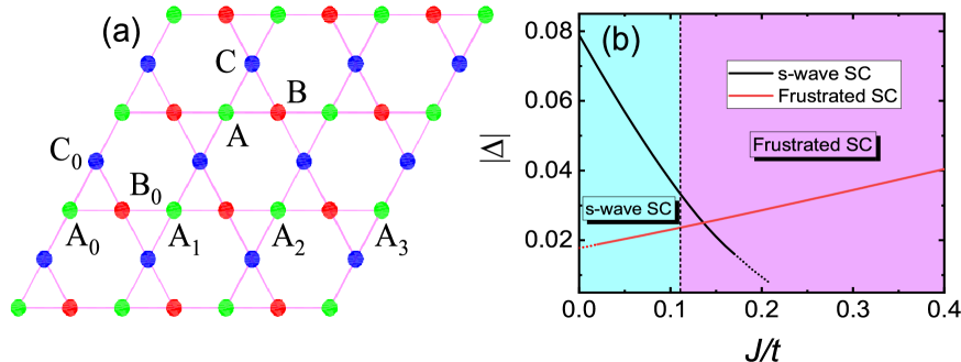
Figure 1: (a) Structure of the kagome lattice, made out of three sublattices A (green dots), B (red dots), and C (blue dots). (b) The SC pairing amplitude as a function of the pairing hopping strength $J$. The light cyan region with $J<0.11$ indicates the conventional $s$-wave SC state, and the light purple region with $J>0.11$ denotes the frustrated SC state.

As a function of the pairing hopping strength $J$, the calculations show that the conventional $s$-wave SC state possesses the lower free energy when $J<0.11$, whereas the frustrated SC state wins over when $J>0.11$. In the conventional $s$-wave SC regime, the pairing hopping tends to suppress the SC pairing amplitude, but in the frustrated SC region the pairing hopping enhances the SC pairing amplitude. The results are displayed in Fig. 1(b), where the vertical dashed line borders the transition between the conventional $s$-wave and frustrated SC states, and the dotted portions in each curves are numerically unreachable in their respective state.

III.2 The structure of the frustrated SC pairing

The SC pairings in the Hamiltonian are defined on the orbital basis, while the spectral experiments usually measure the electronic structures near the Fermi surface, which is certainly on the band basis. To gain the clear picture about the frustrated SC state, we transform the SC pairings into band space through a unitary transformation,

$$\Delta_{mn}(k) = \sum_{\alpha\beta}u^{\ast}_{m\alpha}(k)\Delta_{\alpha\beta}u^{\ast}_{n\beta}(-k),$$ (28)

where $u_{m\alpha}(k)$ and $\Delta_{\alpha\beta}$ are the eigenstates of band $m$ and the SC pairings defined on the orbital basis. The diagonal components of $\Delta_{mn}(k)$ correspond to the intra-band pairing, and the off-diagonal components represent the inter-band pairings. While both the diagonal and the off-diagonal components could be non-zero, the inter-band pairings in this circumstance do not lead to a gap opening at the Fermi level. Meanwhile, the first band $(m=1)$ and third band $(m=3)$ stay away from the Fermi level. Thus, only the diagonal component in the middle band $\Delta_{22}(k)$ is relevant to the experimental measurements.

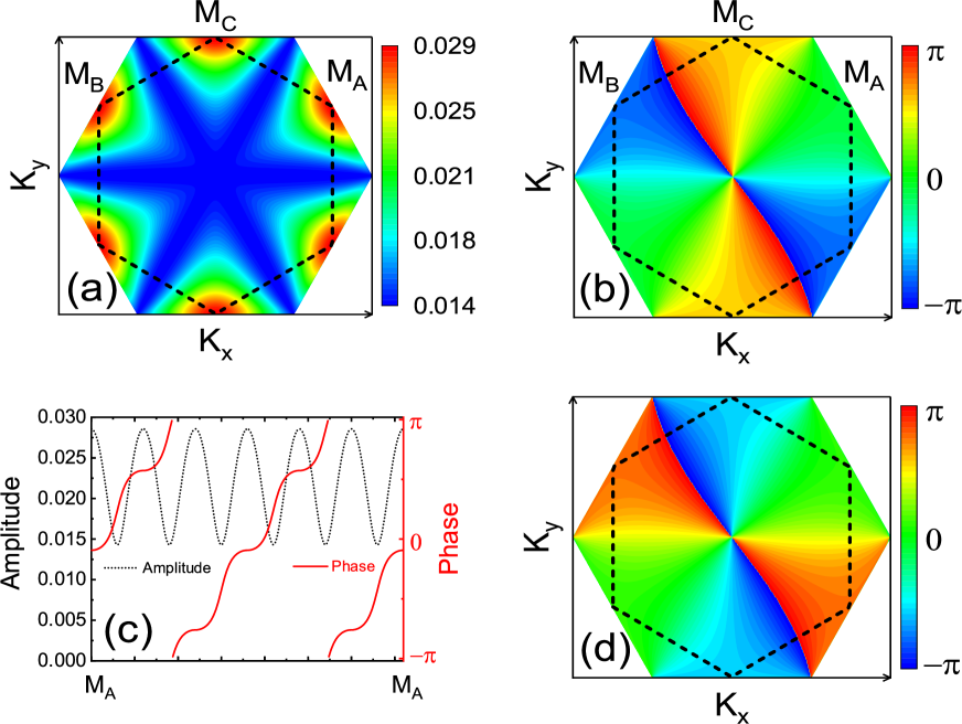
Figure 2: Distributions of the amplitude (a) and phase (b) of the frustrated SC state in the primitive Brillouin zone. (c) Variations of the amplitude and phase of the frustrated SC state following in a counterclockwise direction around the Fermi surface shown as dashed lines in (a) and (b). (d) Same as (b) but with opposite chirality of the SC pairing.

Figs. 2(a) and (b) present respectively the distributions of the amplitude and the phase of $\Delta_{22}(k)$ for the frustrated SC state in primitive Brillouin zone. Fig. 2(c) displays their distributions following a counterclockwise direction around the Fermi surface. Two salient features are observed from the figure. Firstly, while the SC state is fully gaped, the amplitude of the SC pairing modulates along the Fermi surface with six-fold symmetry, which is in line with the recent experimental surveys Roppongi1 . Due the sublattice interference, the van Hove singular points near the van Hove filling come exclusively from the same sublattice sites, and so is the SC pairings. The same phase of the SC pairings on the same sublattice sites gives rise to the maximum $|\Delta|$ at the $M$ points. On the other hand, the midpoint between the two adjacent van Hove points originates from the equally mixing of two inequivalent sublattice sites. This means that $\Delta_{22}(k)$ at the midpoint is derived from the equally mixing of the SC pairings on two inequivalent sublattice sites, i.e., $(|\Delta|+|\Delta|e^{\pm i\frac{2\pi}{3}})/2$ or $(|\Delta|e^{i\frac{2\pi}{3}}+|\Delta|e^{-i\frac{2\pi}{3}})/2$, which produce exactly $|\Delta|/2$ for the minimum of $|\Delta_{22}(k)|$ at the midpoint, just as depicted in Figs. 2(a) and (c). Secondly, depending on the chirality, the phase of the SC pairing undergoes $4\pi$ [Fig. 2(b)] or $-4\pi$ [Fig. 2(d)] changes, i.e., winding of $\pm 2$, when one follow it in a counterclockwise direction around the Fermi surface, explicitly demonstrating the breaking of the time reversal symmetry.

III.3 Conventional aspects of the frustrated SC state

The most notable characteristics in supporting the conventional SC pairing for the kagome superconductors is the observation of the Hebel-Slichter coherent peak in the temperature ($T$) dependence of $(T_{1}T)^{-1}$. In a conventional $s$-wave superconductor, as shown in Fig. 3(a) for the result with $J=0.1$ which leads to the conventional $s$-wave pairing, the $T$ dependence of $(T_{1}T)^{-1}$ develops a peak structure below $T_{c}$, which can be explained theoretically as a result of the nonzero coherent factor described in BCS theory along with the enhancement of the SC DOS at the gap edge. Derivations of $(T_{1}T)^{-1}$ for the Hamiltonian (7) can be found in the Appendix A. In the frustrated SC state, although the amplitude of SC pairing modulates on the Fermi surface and the phase of the SC pairing changes $4\pi$ around the Fermi surface, the phase is the same at each pair of opposite van Hove singularities as displayed in Fig. 2(b), guaranteed by the sublattice interference effect. This in turn leads to a nonzero coherent factor in $(T_{1}T)^{-1}$. As expected, the result with $J=0.2$ shown in Fig.. 3(b) clearly shows the pronounced Hebel-Slichter peak of $(T_{1}T)^{-1}$ just below $T_{c}$. The presence of the Hebel-Slichter peak in the frustrated SC state keeps in line with the corresponding experiments.

In kagome superconductors, another important piece of evidence in favor of conventional SC pairing is the absence of in-gap states near a nonmagnetic impurity. In the presence of impurities, the Hamiltonian should be varied by adding a impurity-scattering term $H_{imp}=\sum_{i,\sigma}U_{i}c^{{\dagger}}_{i\sigma}c_{i\sigma}$ with $U_{i}$ denoting the scattering strength of the impurity on site $i$. In this circumstance, we should transform the Bogoliubov-de Gennes equations in Eq. (11) into the real space as,

$$\sum_{j}\left(\begin{array}[]{cc}H_{ij,\sigma}&\Delta_{ij}\\ \Delta^{\ast}_{ij}&-H^{\ast}_{ij,\bar{\sigma}}\end{array}\right)\left(\begin{array}[]{cc}u_{n,j,\sigma}\\ v_{n,j,\bar{\sigma}}\end{array}\right)=E_{n}\left(\begin{array}[]{cc}u_{n,i,\sigma}\\ v_{n,i,\bar{\sigma}}\end{array}\right),$$ (35)

where $H_{ij,\sigma}=-t_{ij}\delta_{i+\mathbf{\tau}_{j},j}-\mu\delta_{i,j}+U_{i}\delta_{i,j}$ with $\mathbf{\tau}_{j}$ denoting the four NN vectors. $\Delta_{ij}=(\Delta_{i}-\frac{J}{V_{s}}\eta_{i})\delta_{i,j}$ represents the contributions from the on-site SC pairing and pairing hoping. $u_{n,i,\sigma}$ and $v_{n,i,\bar{\sigma}}$ are the Bogoliubov quasiparticle amplitudes on the $i$-th site with corresponding eigenvalue $E_{n}$. The self-consistent equations for the amplitude of the SC pairing $\Delta_{i}$ and the electron density $n_{i}$ on site $i$ can be obtained in the same way as Eq. (14). Then, the local density of state (LDOS) is given by $\rho(E,\mathbf{r}_{i})=-\sum_{n}[|u_{n,i,\uparrow}|^{2}f^{{}^{\prime}}(E_{n}-E)+|v_{n,i,\downarrow}|^{2}f^{{}^{\prime}}(E_{n}+E)]$, which is proportional to the differential tunneling conductance observed in scanning tunneling microscopy (STM) experiments. To diminish the finite size effect, we adopt the supercell technique for the numerical calculations in real space.

We consider the case of one unitary nonmagnetic impurity embodied in the system, which is represented by setting $U_{i}=U_{0}\delta_{i,i_{0}}$ with $U_{0}$ and $i_{0}$ denoting the scattering strength and the location of the impurity. For definition, we choose $U_{0}=50.0$ that is well in the unitary regime and lay the impurity on the $A$ sublattice site as marked by $A_{0}$ in Fig. 1(a). Figs. 3(c) and (d) present respectively the LDOS results for $J=0.1$ and $J=0.2$ in the case of one nonmagnetic impurity.

On the one hand, the bulk density of states (DOS) for $J=0.1$ exhibits a U-shaped profile characteristic of isotropic $s$-wave SC pairing, while the basinlike V-shaped DOS for $J=0.2$ indicates anisotropic yet fully gapped SC pairing, both behaviors aligning with the expectations from Figs. 1(b) and  2(a). Despite these distinct pairing symmetries, neither the isotropic $s$-wave nor the anisotropic frustrated SC state shows significant impurity-induced in-gap states, as evidenced by the absence of such features in Figs. 3(c) and (d). On the other hand, while impurity-induced suppression of the SC gap edges in the LDOS persists over long distances at the same sublattice as the impurity site, it has minimal impact on LDOS at different sublattice sites, even within the same unit cell. This contrast underscores the distinct sublattice interference effect inherent to the kagome system. Owing to sublattice interference, each of the three van Hove singular points ($M_{A},M_{B},M_{C}$) originates exclusively from one of the three inequivalent lattice sites ($A,B,C$). Consequently, an impurity located at a specific sublattice site, e.g., sublattice $A$, primarily scatters electrons near the $M_{A}$ points in reciprocal space, with a corresponding scattering effect observed in real space (See Appendix B for details.). Thus, the impurity exerts a negligible influence on the LDOS across different sublattices. Meanwhile, since the same sublattice sites share identical SC phases, impurity effects primarily manifest as suppression of the SC gap edges at the same sublattice sites without inducing significant shifts of these edges (With the exception of the same sublattice site within the NN unit cell, which exhibits the strongest impurity-induced response.). This behavior is quantitatively captured by curves $A_{2}-A_{5}$ in Figs. 3(c) and (d).

Theoretically, the local electronic structure at the impurity’s NN-site, which usually yield the optimal outcome, are widely utilized to characterize such perturbations. However, in kagome systems, this paradigm requires revision, since the strongest impurity-induced signatures emerge not at the impurity’s NN site, but at the same sublattice of the NN unit cell, as unambiguously demonstrated by the $A_{1}$ curves in Figs. 3(c) and (d).

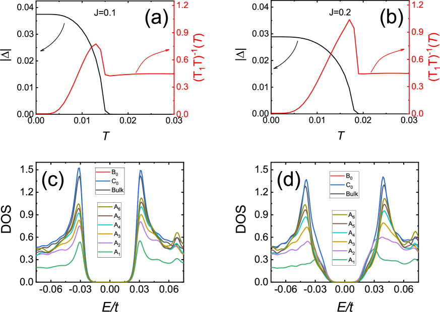
Figure 3: Temperature dependence of the amplitude of SC pairing $|\Delta|$ and $(T_{1}T)^{-1}$ for $J=0.1$ (a) and $J=0.2$ (b). The energy dependence of the DOS on a series of sites for $J=0.1$ (c), and $J=0.2$ (d). In (c) and (d), $B_{0}$ and $C_{0}$ denote the other two sublattice sites within the same unit cell as the impurity site $A_{0}$, and $A_{1}-A_{5}$ stand for the LDOS at the same sublattice sites as the impurity site $A_{0}$ in different unit cell moving away from $A_{0}$ [See Fig. 1(a).].

III.4 Impurity-induced phase transition

Although the frustrated SC state remains insensitive to a strong impurity manifested by the absence of impurity-induced in-gap states, even a weak impurity does depress the SC amplitude $|\Delta_{i}|$ and disturb the SC phase $\theta_{i}$ significantly at the same sublattice sites near the impurity, as revealed in Fig. 4(a). Whereas the SC amplitude $|\Delta_{i}|$ exhibits minor spatial variations across different sublattice sites near the impurity, the SC phase $\theta_{i}$ also demonstrates a pronounced deviation from its equilibrium value in the geometrically frustrated SC state, as shown in Fig. 4(b). These perturbations will locally disrupt the delicate balance among the three adjacent sublattices in the frustrated SC state. Thereby, the collective effects arising from multiple impurities are expected to profoundly modify the global configuration of the frustrated SC state.

To explicitly investigate this phenomenon, we consider the case of random impurities which is defined by an independent random variable $U_{i}$ randomly distributed over $[-W,W]$ at randomly selected half sites $r_{i}$ of the total sites. Then $W$ is a parameter for characterizing the strength of the disorder. For illustration purposes, we define the average phase difference between the sublattices as $\varphi=\frac{1}{4N}\Sigma_{i}[(\theta_{A,i}-\theta_{B,i})+(\theta_{B,i}-\theta_{C,i})+(\theta_{C,i}-\theta_{A,i})]$, and the average amplitude of the SC pairings as $|\bar{\Delta}|=\frac{1}{3N}\Sigma_{\alpha,i}|\Delta_{\alpha,i}|$, where $\theta_{\alpha,i}$ and $N$ stand for respectively the phase of the SC pairing on sublattice $(\alpha,i)$ and the number of the total unit cells used in the calculations. Obviously, $\varphi$ should be equal or approach to $\frac{2\pi}{3}$ if the system is in the frustrated SC state, and should be zero if it is in the conventional $s$-wave state. Fig. 4(c) presents the disorder strength $W$ dependence of the phase difference $\varphi$ and the average amplitude $\bar{\Delta}$ for specific values of $J=0.13$ and $J=0.14$. As clearly shown in the figure, while $|\bar{\Delta}|$ exhibits a steady but weak decrease with disorder, the phase difference $\varphi$ switches from $2\pi/3$ to zero at $W=0.25$ for $J=0.13$ and at $W=0.35$ for $J=0.14$. Accordingly, as displayed in Fig. 4(d), the DOS undergoes a transition from the basinlike V-shaped DOS at weak disorder to the U-shaped one at strong disorder, portraying an impurity-induced SC pairing transition from the anisotropic time-reversal symmetry breaking SC state to the conventional $s$-wave SC state without passing through the nodal point. It is worth noting that the disorder-induced SC pairing transition mirrors the quintessential feature of the experimental observation Roppongi1 .

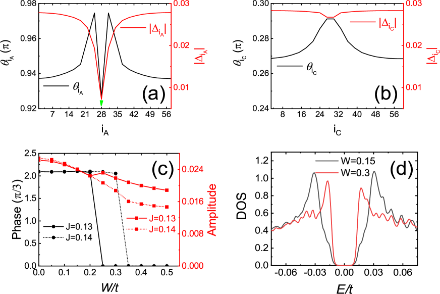
Figure 4: Spatial distributions of SC amplitude $|\Delta_{i}|$ and phase $\theta_{i}$ on the $A$-sublattice sites (a), and on the $B$-sublattice sites (b), where a $U_{0}=2$ impurity is embedded at the $A$-sublattice site indicated by the short green arrow in (a). (c) The average phase difference $\varphi$ between the sublattices and the average amplitude of the SC pairings $|\bar{\Delta}|$ as a function of the impurity strength $W$. (d) The energy dependence of the average DOS at different $W$ for $J=0.13$.

III.5 Discussion

The AV₃Sb₅ superconductors, which are kagome lattices near the van Hove filling, would be the promising system for realizing the frustrated superconductivity outline here. In these systems, the sublattice interference near the van Hove singularity has a pronounced effect on reducing the on-site interaction relative to nearest neighbor interactions Kiesel3 . This subsequently facility the nearest neighbor Cooper pair hoppings in the superconductors, which is precisely the requisite condition for the frustrated superconductivity identified here.

The pair hopping interaction on the square lattice has been proposed earlier to account for the $\eta$-type pairing phase where the total momentum of the paired electrons is $Q=(\pi,\pi)$ and the phase of SC order parameter alters from one site to the neighboring one Penson1 ; Bulka1 ; Czart1 ; Czart2 ; Japar1 . It was shown that flux quantization and Meissner effect appear in this state Yang1 ; Yang2 . On the contrary, the alterations of the SC phase between the three sublattices for the kagome lattice do not break the translational symmetry, so the momentum of the SC pairing still remains zero, just like the traditional SC state. Nevertheless, the alteration of the SC phase causes the frustrated superconductivity which simultaneously breaks time-reversal symmetry.

In a specific case, if we assign the phases $e^{-i2\pi/3}$, $1$ and $e^{i2\pi/3}$ to the SC order parameters on the three sublattice sites $A$, $B$ and $C$, respectively. In sublattice space, the SC pairings can be written in the following matrix form,

$$\left(\begin{array}[]{ccc}\Delta e^{-i\frac{2\pi}{3}}&0&0\\ 0&\Delta&0\\ 0&0&\Delta e^{i\frac{2\pi}{3}}\end{array}\right),$$ (39)

which is in turn decoupled into the real and imaginary parts as,

$$\frac{1}{2}\left(\begin{array}[]{ccc}-\Delta&0&0\\ 0&2\Delta&0\\ 0&0&-\Delta\end{array}\right)+i\frac{\sqrt{3}}{2}\left(\begin{array}[]{ccc}-\Delta&0&0\\ 0&0&0\\ 0&0&\Delta\end{array}\right).$$ (46)

This equivalents to the pairing symmetry of $E^{(1)}_{2}+iE^{(2)}_{2}$ used in Ref. Holb1, up to a global phase factor $e^{i\pi}$.

IV Conclusion

In conclusion, we have proposed a theory to explore the possible frustrated SC state in the kagome superconductors. It is revealed in this theory that the frustrated SC state emerges as a result of the symmetry mismatch between the conventional $s$-wave SC pairing and the crystal lattice when the NN-sites Cooper pairing hoping was considered. In this state, the SC pairing on the three sublattices has $2\pi/3$ phase difference from each other, leading to the six-fold modulation of the amplitude and the time-reversal symmetry breaking with $4\pi$ phase changes of the SC pairing as one following it around the Fermi surface. In this state, the SC pairing on the three sublattices exhibits a mutual $2\pi/3$ phase difference. This phase arrangement leads to a six-fold modulation of the SC order parameter amplitude and induces time-reversal symmetry breaking through a $4\pi$ phase winding of the SC pairing when traversing a closed path along the Fermi surface. On the other hand, the frustrated SC state manifests a pronounced Hebel-Slichter coherence peak in the nuclear spin-lattice relaxation rate below $T_{c}$, and avoids impurity-induced in-gap states.In particular, the theory also revealed a disorder-induced SC pairing transition from the frustrated SC state to an isotropic $s$-wave SC state without passing through the nodal point, a process that aligns with and explains experimental observations. This theory not only offered a promising framework to reconcile divergent or seemingly contradictory experimental observations regarding SC properties, but might also set the foundation for investigating geometrically frustrated SC states in kagome lattice materials.

V acknowledgement

This work was supported by the National Key Projects for Research and Development of China (No. 2024YFA1408104) and the National Natural Science Foundation of China (No. 12374137, and No. 12434005).

Appendix A Derivation of the spin-lattice relaxation rate

The spin-lattice relaxation rate $\frac{1}{T_{1}T}$ is related to the imaginary part of spin susceptibility,

$$\frac{1}{T_{1}T} \propto \lim_{\omega\rightarrow 0}\frac{1}{N}\sum_{\mathbf{q}}\textmd{Im}\frac{\chi_{0}^{+-}(\omega,\mathbf{q})}{\omega}.$$ (47)

Here, $\chi_{0}^{+-}(\omega,\mathbf{q})=\int_{0}^{\beta}d\tau e^{i\omega\tau}\chi_{0}^{+-}(\tau,\mathbf{q})$ with $\chi_{0}^{+-}(\tau,\mathbf{q})$ defined as,

$$\chi_{0}^{+-}(\tau,\mathbf{q}) = \frac{1}{N}\langle T_{\tau}S_{\mathbf{q}}^{+}(\tau)S_{-\mathbf{q}}^{-}(0)\rangle,$$ (48)

where $S_{\mathbf{q}}^{+}=\Sigma_{l,\mathbf{k}}c_{l,\mathbf{k}+\mathbf{q},\uparrow}^{\dagger}c_{l,\mathbf{k},\downarrow}$ and $S_{\mathbf{-q}}^{-}=(S_{\mathbf{q}}^{+})^{\dagger}$. Resorting to the Wick’s theorem and making the Bogoliubov transformations $c_{l,\mathbf{k},\uparrow}=\sum_{n}[u_{ln}(\mathbf{k})\gamma_{n\uparrow}(\mathbf{k})-v_{ln}^{\ast}(\mathbf{k})\gamma_{n\downarrow}^{\dagger}(-\mathbf{k})]$ and $c_{l,-\mathbf{k},\downarrow}=\sum_{n}[u_{ln}(\mathbf{k})\gamma_{n\downarrow}(-\mathbf{k})+v_{ln}^{\ast}(\mathbf{k})\gamma_{n\uparrow}^{\dagger}(\mathbf{k})]$, we finally arrive at the following expression of $\chi_{0}^{+-}(\omega,\mathbf{q})$,

$$\chi_{0}^{+-}(\omega,\mathbf{q})= \frac{1}{N}\sum_{l\lambda,nm,\mathbf{k}}[(u_{l,n,\mathbf{k}+\mathbf{q}}^{\ast}u_{\lambda,n,\mathbf{k}+\mathbf{q}}v_{l,m,\mathbf{k}}^{\ast}v_{\lambda,m,\mathbf{k}}-u_{l,n,\mathbf{k}+\mathbf{q}}^{\ast}v_{\lambda,n,\mathbf{k}+\mathbf{q}}v_{l,m,\mathbf{k}}^{\ast}u_{\lambda,m,\mathbf{k}})\frac{1-f(E_{n,\mathbf{k}+\mathbf{q}})-f(E_{m,\mathbf{k}})}{\omega+E_{n,\mathbf{k}+\mathbf{q}}+E_{m,\mathbf{k}}+i\delta}$$ (49)

$$+(v_{l,n,\mathbf{k}+\mathbf{q}}v_{\lambda,n,\mathbf{k}+\mathbf{q}}^{\ast}v_{l,m,\mathbf{k}}^{\ast}v_{\lambda,m,\mathbf{k}}+v_{l,n,\mathbf{k}+\mathbf{q}}u_{\lambda,n,\mathbf{k}+\mathbf{q}}^{\ast}v_{l,m,\mathbf{k}}^{\ast}u_{\lambda,m,\mathbf{k}})\frac{f(E_{n,\mathbf{k}+\mathbf{q}})-f(E_{m,\mathbf{k}})}{\omega-E_{n,\mathbf{k}+\mathbf{q}}+E_{m,\mathbf{k}}+i\delta}$$

$$+(u_{l,n,\mathbf{k}+\mathbf{q}}^{\ast}u_{\lambda,n,\mathbf{k}+\mathbf{q}}u_{l,m,\mathbf{k}}u_{\lambda,m,\mathbf{k}}+u_{l,n,\mathbf{k}+\mathbf{q}}^{\ast}v_{\lambda,n,\mathbf{k}+\mathbf{q}}u_{l,m,\mathbf{k}}v_{\lambda,m,\mathbf{k}}^{\ast})\frac{f(E_{m,\mathbf{k}})-f(E_{n,\mathbf{k}+\mathbf{q}})}{\omega-E_{m,\mathbf{k}}+E_{n,\mathbf{k}+\mathbf{q}}+i\delta}$$

$$+(v_{l,n,\mathbf{k}+\mathbf{q}}v_{\lambda,n,\mathbf{k}+\mathbf{q}}^{\ast}u_{l,m,\mathbf{k}}u_{\lambda,m,\mathbf{k}}^{\ast}-v_{l,n,\mathbf{k}+\mathbf{q}}u_{\lambda,n,\mathbf{k}+\mathbf{q}}^{\ast}u_{l,m,\mathbf{k}}v_{\lambda,m,\mathbf{k}}^{\ast})\frac{f(E_{n,\mathbf{k}+\mathbf{q}})+f(E_{m,\mathbf{k}})-1}{\omega-E_{n,\mathbf{k}+\mathbf{q}}-E_{m,\mathbf{k}}+i\delta}].$$

Appendix B Sublattice interference effect on the impurity state

The observed sublattice dichotomy, where impurity-induced states strongly localize on the host sublattice while leaving the LDOS on the adjacent sublattice nearly intact, is qualitatively explained by the $T$-matrix formalism through sublattice interference processes.

Within the $T$-matrix framework, the impurity-renormalized Green’s function at site $\mathbf{r}$ is formally expressed as,

$$\hat{G}(\mathbf{r},\mathbf{r},i\omega_{n}) = \hat{G}_{0}(\mathbf{r}-\mathbf{r},i\omega)+\hat{G}_{0}(\mathbf{r}-\mathbf{r}_{0},i\omega)\hat{T}(\mathbf{r}_{0},i\omega)\hat{G}_{0}(\mathbf{r}_{0}-\mathbf{r},i\omega),$$ (50)

where $\hat{G}_{0}(i\omega)$ denotes the bare Green’s function, and the $\hat{T}(\mathbf{r}_{0},i\omega)$-matrix encapsulates the full scattering sequence through the Dyson series,

$$\hat{T}(\mathbf{r}_{0},i\omega) = \frac{\hat{V}}{\hat{1}-\hat{V}\hat{G}_{0}(\mathbf{r}_{0},i\omega)}.$$ (51)

Here, $\hat{V}=V_{0}\hat{\tau}_{3}$ accounts for the potential impurity at location $\mathbf{r}_{0}$. Then, the LDOS at site $\mathbf{r}$ is expressed as $\rho(E,\mathbf{r})=-\frac{1}{\pi}\textmd{Im}[\hat{G}_{ee}(\mathbf{r},\mathbf{r},\omega_{n}+i\delta)+\hat{G}_{hh}(\mathbf{r},\mathbf{r},-\omega_{n}+i\delta)]$, where the diagonal elements $\hat{G}_{ee}$ and $\hat{G}_{hh}$ correspond to the contributions from the electron and hole parts, respectively.

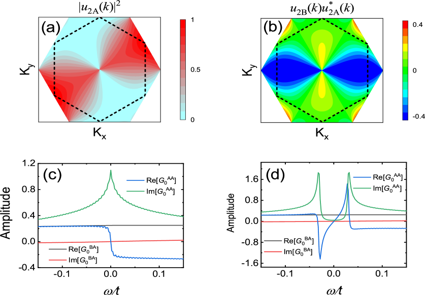
Figure B1: The momentum distribution of the form factors $|u_{2,A}(\mathbf{k})|^{2}$ (a), and $u_{2,B}(\mathbf{k})u_{2,A}^{\ast}(\mathbf{k})$ (b), respectively. Real and imaginary parts of the Green’s functions $\hat{G}_{0,ee}^{AA}(\mathbf{r}_{A_{1}}-\mathbf{r}_{A_{0}},\omega+i\delta)$ and $\hat{G}_{0,ee}^{BA}(\mathbf{r}_{B_{0}}-\mathbf{r}_{A_{0}},\omega+i\delta)$ for the normal state (c), and for the SC state (d). $\hat{G}_{0,ee}^{AA}(\mathbf{r}_{A_{1}}-\mathbf{r}_{A_{0}},\omega+i\delta)$ and $\hat{G}_{0,ee}^{BA}(\mathbf{r}_{B_{0}}-\mathbf{r}_{A_{0}},\omega+i\delta)$ have been abbreviated respectively as $\hat{G}_{0}^{AA}$ and $\hat{G}_{0}^{BA}$ in the figures.

For an impurity with a given strength located on a specific sublattice site $A$ at location $\mathbf{r}_{A_{0}}$, the Green’s functions at the same sublattice $A$ at location $\mathbf{r}_{A}$ is expressed as

$$\hat{G}^{AA}(\mathbf{r}_{A},\mathbf{r}_{A},i\omega_{n}) = \hat{G}_{0}^{AA}(\mathbf{r}_{A}-\mathbf{r}_{A},i\omega)+\hat{G}_{0}^{AA}(\mathbf{r}_{A}-\mathbf{r}_{A_{0}},i\omega)\hat{T}(\mathbf{r}_{A_{0}},i\omega)\hat{G}_{0}^{AA}(\mathbf{r}_{A_{0}}-\mathbf{r}_{A},i\omega),$$ (52)

while the Green’s functions at another sublattice $B$ at location $\mathbf{r}_{B}$ is expressed as

$$\hat{G}^{BB}(\mathbf{r}_{B},\mathbf{r}_{B},i\omega_{n}) = \hat{G}_{0}^{BB}(\mathbf{r}_{B}-\mathbf{r}_{B},i\omega)+\hat{G}_{0}^{BA}(\mathbf{r}_{B}-\mathbf{r}_{A_{0}},i\omega)\hat{T}(\mathbf{r}_{A_{0}},i\omega)\hat{G}_{0}^{AB}(\mathbf{r}_{A_{0}}-\mathbf{r}_{B},i\omega).$$ (53)

Both the bare Green’s functions $\hat{G}_{0}^{AA/BB}(\mathbf{r}_{A/B}-\mathbf{r}_{A/B},i\omega)$ and the $\hat{T}(\mathbf{r}_{0}=\mathbf{r}_{A_{0}},i\omega)$-matrix in Eqs. (A3) and (A4) are the same, so the difference comes from $\hat{G}_{0}^{AA}(\mathbf{r}_{A}-\mathbf{r}_{A_{0}},i\omega)$ and $\hat{G}_{0}^{BA}(\mathbf{r}_{B}-\mathbf{r}_{A_{0}},i\omega)$. For simplicity, we only consider the electron part of $\hat{G}_{0}(i\omega)$ in the following.

$$\hat{G}_{0,ee}^{l\lambda}(\mathbf{r}-\mathbf{r}_{0},i\omega)=-\int_{0}^{\beta}e^{i\omega\tau}d\tau\langle T_{\tau}c_{l,\mathbf{r}}^{{\dagger}}(\tau)c_{\lambda,\mathbf{r}_{0}}(0)\rangle.$$ (54)

After making the transformations $c_{\lambda,\mathbf{r}}=\sum_{k}c_{\lambda,\mathbf{k}}e^{i\mathbf{k}\cdot\mathbf{r}}$ and $c_{\lambda,\mathbf{k}}=\sum_{n}u_{n,\lambda}^{\ast}(\mathbf{k})\phi_{n}(\mathbf{k})$, we finally arrive at,

$$\hat{G}_{0,ee}^{AA}(\mathbf{r}_{A}-\mathbf{r}_{A_{0}},i\omega)=\sum_{n,\mathbf{k}}\frac{|u_{n,A}(\mathbf{k})|^{2}}{i\omega-\varepsilon_{n}(\mathbf{k})}e^{-i\mathbf{k}\cdot(\mathbf{r}_{A}-\mathbf{r}_{A_{0}})},$$ (55)

and

$$\hat{G}_{0,ee}^{BA}(\mathbf{r}_{B}-\mathbf{r}_{A_{0}},i\omega)=\sum_{n,\mathbf{k}}\frac{u_{n,B}(\mathbf{k})u_{n,A}^{\ast}(\mathbf{k})}{i\omega-\varepsilon_{n}(\mathbf{k})}e^{-i\mathbf{k}\cdot(\mathbf{r}_{B}-\mathbf{r}_{A_{0}})}.$$ (56)

Since the band $2$ crosses the Fermi energy, the form factors $|u_{2,A}(\mathbf{k})|^{2}$ and $u_{2,B}(\mathbf{k})u_{2,A}^{\ast}(\mathbf{k})$ are dominant in Eqs. (B6) and (B7). Figs. B1(a) and (b) presents the momentum distribution of the form factors $|u_{2,A}(\mathbf{k})|^{2}$ and $u_{2,B}(\mathbf{k})u_{2,A}^{\ast}(\mathbf{k})$.

Owing to the sublattice interference effect, the form factor $|u_{2,A}(\mathbf{k})|^{2}$ peaks predominantly around van Hove singularities, reaching maximal intensity precisely at these critical points. The overlapping of the two factors will boost the Green’s function $\hat{G}_{0,ee}^{AA}(\mathbf{r}_{A}-\mathbf{r}_{A_{0}},\omega+i\delta)$ to a significant changes near the Fermi energy for the normal state and near the gap edge for the SC state, as shown in Fig. B1(c) and (d) for the Green’s functions between the impurity and the same sublattice of the NN-unit cell $\hat{G}_{0,ee}^{AA}(\mathbf{r}_{A_{1}}-\mathbf{r}_{A_{0}},\omega+i\delta)$. On the contrary, the form factor $u_{2,B}(\mathbf{k})u_{2,A}^{\ast}(\mathbf{k})$ is zero along most part of the Fermi surface except for the segments crossing the blue regions, exactly avoiding the van Hove singularities. The coincidence of the nonzero form factor and low DOS segments of the Fermi surface causes featureless for the Green’s function $\hat{G}_{0,ee}^{BA}(\mathbf{r}_{B}-\mathbf{r}_{A_{0}},i\omega)$, as displayed in Fig. B1(c) and (d) for the Green’s functions between the impurity and its NN $B$ sublattice site $\hat{G}_{0,ee}^{BA}(\mathbf{r}_{B_{0}}-\mathbf{r}_{A_{0}},\omega+i\delta)$. Therefor, the impurity produces the strongest impurity-induced response at the same sublattice site in the NN unit cell, while it exerts a negligible influence on the LDOS across different sublattices.

References

- (1) B. R. Ortiz, S. M. L. Teicher, Y. Hu, J. L. Zuo, P. M. Sarte, E. C. Schueller, A. M. M. Abeykoon, M. J. Krogstad, S. Rosenkranz, R. Osborn, R. Seshadri, L. Balents, J. He, and S. D. Wilson, Phys. Rev. Lett. 125, 247002 (2020).
- (2) Y.-X. Jiang, J.-X. Yin, M. M. Denner, N. Shumiya, B. R. Ortiz, G. Xu, Z. Guguchia, J. He, M. S. Hossain, X. Liu, J. Ruff, L. Kautzsch, S. S. Zhang, G. Chang, I. Belopolski, Q. Zhang, T. A. Cochran, D. Multer, M. Litskevich, Z.-J. Cheng, X. P. Yang, Z. Wang, R. Thomale, T. Neupert, S. D. Wilson, and M. Z. Hasan, Nat. Mater. 20, 1353 (2021).
- (3) H. Chen, H. Yang, B. Hu, Z. Zhao, J. Yuan, Y. Xing, G. Qian, Z. Huang, G. Li, Y. Ye, S. Ma, S. Ni, H. Zhang, Q. Yin, C. Gong, Z. Tu, H. Lei, H. Tan, S. Zhou, C. Shen, X. Dong, B. Yan, Z. Wang, and H.-J. Gao, Nature 599, 222 (2021).
- (4) Z. Liang, X. Hou, F. Zhang, W. Ma, P. Wu, Z. Zhang, F. Yu, J.-J. Ying, K. Jiang, L. Shan, Z. Wang, and X.-H. Chen, Phys. Rev. X 11, 031026 (2021).
- (5) H. Li, T. T. Zhang, T. Yilmaz, Y. Y. Pai, C. E. Marvinney, A. Said, Q. W. Yin, C. S. Gong, Z. J. Tu, E. Vescovo, C. S. Nelson, R. G. Moore, S. Murakami, H. C. Lei, H. N. Lee, B. J. Lawrie, and H. Miao, Phys. Rev. X 11, 031050 (2021).
- (6) C. Mielke III, D. Das, J.-X. Yin, H. Liu, R. Gupta, Y.-X. Jiang, M. Medarde, X. Wu, H. C. Lei, J. Chang, P. Dai, Q. Si, H. Miao, R. Thomale, T. Neupert, Y. Shi, R. Khasanov, M. Z. Hasan, H. Luetkens, and Z. Guguchia, Nature 602, 245 (2022).
- (7) F. H. Yu, T. Wu, Z. Y. Wang, B. Lei, W. Z. Zhuo, J. J. Ying, and X. H. Chen, Phys. Rev. B 104, L041103 (2021).
- (8) N. Shumiya, Md. S. Hossain, J.-X. Yin, Y.-X. Jiang, B. R. Ortiz, H. Liu, Y. Shi, Q. Yin, H. Lei, S. S. Zhang, G. Chang, Q. Zhang, T. A. Cochran, D. Multer, M. Litskevich, Z.-J. Cheng, X. P. Yang, Z. Guguchia, S. D. Wilson, and M. Z. Hasan, Phys. Rev. B 104, 035131 (2021).
- (9) C. Guo, C. Putzke, S. Konyzheva, X. Huang, M. Gutierrez-Amigo, I. Errea, D. Chen, M. G. Vergniory, C. Felser, M. H. Fischer, T. Neupert, and P. J. W. Moll, Nature 611, 461 (2022).
- (10) S.-Y. Yang, Y. Wang, B. R. Ortiz, D. Liu, J. Gayles, E. Derunova, R. Gonzalez-Hernandez, L. Šmejkal, Y. Chen, S. S. P. Parkin, S. D. Wilson, E. S. Toberer, T. McQueen, and M. N. Ali, Sci. Adv. 6, eabb6003 (2020).
- (11) B. R. Ortiz, P. M. Sarte, E. M. Kenney, M. J. Graf, S. M. L. Teicher, R. Seshadri, and S. D. Wilson, Phys. Rev. Mater. 5, 034801 (2021).
- (12) Q. Yin, Z. Tu, C. Gong, Y. Fu, S. Yan, and H. Lei, Chin. Phys. Lett. 38, 037403 (2021).
- (13) K. Y. Chen, N. N. Wang, Q. W. Yin, Y. H. Gu, K. Jiang, Z. J. Tu, C. S. Gong, Y. Uwatoko, J. P. Sun, H. C. Lei, J. P. Hu, and J.-G. Cheng, Phys. Rev. Lett. 126, 247001 (2021).
- (14) Z. Zhang, Z. Chen, Y. Zhou, Y. Yuan, S. Wang, J. Wang, H. Yang, C. An, L. Zhang, X. Zhu, Y. Zhou, X. Chen, J. Zhou, and Z. Yang, Phys. Rev. B 103, 224513 (2021).
- (15) X. Chen, X. Zhan, X. Wang, J. Deng, X.-B. Liu, X. Chen, J.-G. Guo, and X. Chen, Chin. Phys. Lett. 38, 057402 (2021).
- (16) H.-S. Xu, Y.-J. Yan, R. Yin, W. Xia, S. Fang, Z. Chen, Y. Li, W. Yang, Y. Guo, and D.-L. Feng, Phys. Rev. Lett. 127, 187004 (2021).
- (17) C. Mu, Q. Yin, Z. Tu, C. Gong, H. Lei, Z. Li, and J. Luo, Chin. Phys. Lett. 38, 077402 (2021).
- (18) W. Duan, Z. Nie, S. Luo, F. Yu, B. R. Ortiz, L. Yin, H. Su, F. Du, A. Wang, Y. Chen, X. Lu, J. Ying, S. D. Wilson, X. Chen, Y. Song, and H. Yuan, Sci. China-Phys. Mech. Astron. 64, 107462 (2021).
- (19) C. C. Zhao, L. S. Wang, W. Xia, Q. W. Yin, J. M. Ni, Y. Y. Huang, C. P. Tu, Z. C. Tao, Z. J. Tu, C. S. Gong, H. C. Lei, Y. F. Guo, X. F. Yang, and S. Y. Li, arXiv: 2102.08356.
- (20) S. Ni, S. Ma, Y. Zhang, J. Yuan, H. Yang, Z. Lu, N. Wang, J. Sun, Z. Zhao, D. Li, S. Liu, H. Zhang, H. Chen, K. Jin, J. Cheng, L. Yu, F. Zhou, X. Dong, J. Hu, H.-J. Gao, and Z. Zhao, Chin. Phys. Lett. 38, 057403 (2021).
- (21) Y. Xiang, Q. Li, Y. Li, W. Xie, H. Yang, Z. Wang, Y. Yao, and H.-H. Wen, Nat. Commun. 12, 6727 (2021).
- (22) B. R. Ortiz, S. M. L. Teicher, L. Kautzsch, P. M. Sarte, N. Ratcliff, J. Harter, J. P. C. Ruff, R. Seshadri, and S. D. Wilson, Phys. Rev. X 11, 041030 (2021).
- (23) X. Zhou, Y. Li, X. Fan, J. Hao, Y. Dai, Z. Wang, Y. Yao, and H.-H. Wen, Phys. Rev. B 104, L041101 (2021).
- (24) M. Kang, S. Fang, J.-K. Kim, B. R. Ortiz, S. H. Ryu, J. Kim, J. Yoo, G. Sangiovanni, D. D. Sante, B.-G. Park, C. Jozwiak, A. Bostwick, E. Rotenberg, E. Kaxiras, S. D. Wilson, J.-H. Park, and R. Comin, Nat. Phys. 18, 301 (2022).
- (25) Y. Fu, N. Zhao, Z. Chen, Q. Yin, Z. Tu, C. Gong, C. Xi, X. Zhu, Y. Sun, K. Liu, and H. Lei, Phys. Rev. Lett. 127, 207002 (2021).
- (26) Y. Song, T. Ying, X. Chen, X. Han, X. Wu, A. P. Schnyder, Y. Huang, J.-g. Guo, and X. Chen, Phys. Rev. Lett. 127, 237001 (2021).
- (27) H. Tan, Y. Liu, Z. Wang, and B. Yan, Phys. Rev. Lett. 127, 046401 (2021).
- (28) F. H. Yu, D. H. Ma, W. Z. Zhuo, S. Q. Liu, X. K. Wen, B. Lei, J. J. Ying, and X. H. Chen, Nat. Commun. 12, 3645 (2021).
- (29) L. Yin, D. Zhang, C. Chen, G. Ye, F. Yu, B. R. Ortiz, S. Luo, W. Duan, H. Su, J. Ying, S. D. Wilson, X. Chen, H. Yuan, Y. Song, and X. Lu, Phys. Rev. B 104, 174507 (2021).
- (30) K. Nakayama, Y. Li, T. Kato, M. Liu, Z. Wang, T. Takahashi, Y. Yao, and T. Sato, Phys. Rev. B 104, L161112 (2021).
- (31) K. Jiang, T. Wu, J.-X. Yin, Z. Wang, M. Z. Hasan, S. D. Wilson, X. Chen, and J. Hu, arXiv: 2109.10809.
- (32) L. Nie, K. Sun, W. Ma, D. Song, L. Zheng, Z. Liang, P. Wu, F. Yu, J. Li, M. Shan, D. Zhao, S. Li, B. Kang, Z. Wu, Y. Zhou, K. Liu, Z. Xiang, J. Ying, Z. Wang, T. Wu, and X. Chen, Nature 604, 59 (2022).
- (33) H. Luo, Q. Gao, H. Liu, Y. Gu, D. Wu, C. Yi, J. Jia, S. Wu, X. Luo, Y. Xu, L. Zhao, Q. Wang, H. Mao, G. Liu, Z. Zhu, Y. Shi, K. Jiang, J. Hu, Z. Xu, and X. J. Zhou, Nat. Commun. 13, 273 (2022).
- (34) T. Neupert, M. M. Denner, J.-X. Yin, R. Thomale, and M. Z. Hasan, Nat. Phys. 18, 137 (2022).
- (35) K. Nakayama, Y. Li, T. Kato, M. Liu, Z. Wang, T. Takahashi, Y. Yao, and T. Sato, Phys. Rev. X 12, 011001 (2022).
- (36) H. Li, S. Wan, H. Li, Q. Li, Q. Gu, H. Yang, Y. Li, Z. Wang, Y. Yao, and H.-H. Wen, Phys. Rev. B 105, 045102 (2022).
- (37) H. Li, H. Zhao, B. R. Ortiz, Y. Oey, Z. Wang, S. D. Wilson, and I. Zeljkovic, Nat. Phys. 19, 637 (2023).
- (38) H. Zhao, H. Li, B. R. Ortiz, S. M. L. Teicher, T. Park, M. Ye, Z. Wang, L. Balents, S. D. Wilson, and I. Zeljkovic, Nature 599, 216 (2021).
- (39) X. Wu, T. Schwemmer, T. Müller, A. Consiglio, G. Sangiovanni, D. Di Sante, Y. Iqbal, W. Hanke, A. P. Schnyder, M. M. Denner, M. H. Fischer, T. Neupert, and R. Thomale, Phys. Rev. Lett. 127, 177001 (2021).
- (40) M. M. Denner, R. Thomale, and T. Neupert, Phys. Rev. Lett. 127, 217601 (2021).
- (41) S. Cho, H. Ma, W. Xia, Y. Yang, Z. Liu, Z. Huang, Z. Jiang, X. Lu, J. Liu, Z. Liu, J. Li, J. Wang, Y. Liu, J. Jia, Y. Guo, J. Liu, and D. Shen, Phys. Rev. Lett. 127, 236401 (2021).
- (42) Y.-P. Lin and R. M. Nandkishore, Phys. Rev. B 106, L060507 (2022).
- (43) L. Zheng, Z. Wu, Y. Yang, L. Nie, M. Shan, K. Sun, D. Song, F. Yu, J. Li, D. Zhao, S. Li, B. Kang, Y. Zhou, K. Liu, Z. Xiang, J. Ying, Z. Wang, T. Wu, and X. Chen, Nature 611, 682 (2022).
- (44) C. Wen, X. Zhu, Z. Xiao, N. Hao, R. Mondaini, H.-M. Guo, and S. Feng, Phys. Rev. B 105, 075118 (2022).
- (45) R. Tazai, Y. Yamakawa, S. Onari, and H. Kontani, Sci. Adv. 8, eabl4108 (2022).
- (46) H.-M. Jiang, S.-L. Yu, and X.-Y. Pan, Phys. Rev. B 106, 014501 (2022).
- (47) Z. Liu, N. Zhao, Q. Yin, C. Gong, Z. Tu, M. Li, W. Song, Z. Liu, D. Shen, Y. Huang, K. Liu, H. Lei, and S. Wang, Phys. Rev. X 11, 041010 (2021).
- (48) Y. Wang, S. Yang, P. K. Sivakumar, B. R. Ortiz, S. M. L. Teicher, H. Wu, A. K. Srivastava, C. Garg, D. Liu, S. S. P. Parkin, E. S. Toberer, T. McQueen, S. D.Wilson, M. N. Ali, Sci. Adv. 9, eadg7269 (2023).
- (49) Y. Zhong, J. Liu, X. Wu, Z. Guguchia, J.-X. Yin, A. Mine, Y. Li, S. Najafzadeh, D. Das, C. Mielke III, R. Khasanov, H. Luetkens, T. Suzuki, K. Liu, X. Han, T. Kondo, J. Hu, S. Shin, Z. Wang, X. Shi, Y. Yao, and K. Okazaki, Nature 617, 488 (2023).
- (50) M. Roppongi, K. Ishihara, Y. Tanaka, et al., Nat. Commun. 14, 667 (2023).
- (51) Y. Wu, Q. Wang, X. Zhou, et al., npj Quantum Mater. 7, 105 (2022).
- (52) Y. Xie, N. Chalus, Z. Wang, et al., Nat. Commun. 15, 6467 (2024).
- (53) S.-L. Yu and J.-X. Li, Phys. Rev. B 85, 144402 (2012).
- (54) W.-S. Wang, Z.-Z. Li, Y.-Y. Xiang, and Q.-H. Wang, Phys. Rev. B 87, 115135 (2013).
- (55) T. Han, J. Che, C. Ye, and H. Huang, Crystals 13, 321 (2023).
- (56) M. L. Kiesel and R. Thomale, Phys. Rev. B 86, 121105(R) (2012).
- (57) J. Liu and T. Zhou, Phys. Rev. B 109, 054504 (2024).
- (58) Y. Gu, Y. Zhang, X. Feng, K. Jiang, and J. Hu, Phys. Rev. B 105, L100502 (2022).
- (59) H.-M. Jiang, M. Mao, Z.-Y. Miao, S.-L. Yu, and J.-X. Li, Phys. Rev. B 109, 104512 (2024).
- (60) H.-M. Jiang, M.-X. Liu, and S.-L. Yu, Phys. Rev. B 107, 064506 (2023).
- (61) X. Lin, J. Huang, and T. Zhou, Phys. Rev. B 110, 134502 (2024).
- (62) T. Le, Z. Pan, Z. Xu, J. Liu, J. Wang, Z. Lou, X. Yang, Z. Wang, Y. Yao, C. Wu, and X. Lin, Nature 630, 64 (2024).
- (63) H. Deng, G. Liu, Z. Guguchia, et al., Nat. Mater. 23, 1639 (2024).
- (64) K. A. Penson and M. Kolb, Phys. Rev. B 33, 1663 (1986).
- (65) S. Robaszkiewicz and B. R. Bulka, Phys. Rev. B 59, 6430 (1999).
- (66) W. R. Czart and S. Robaszkiewicz, Phys. Rev. B 64, 104511 (2001).
- (67) W. R. Czart, S. Robaszkiewicz, and B. Tobijaszewska, Phys. Status Solidi B 244, 2327 (2007).
- (68) G. I. Japaridze, A. P. Kampf, M. Sekania, P. Kakashvili, and Ph Brune, Phys. Rev. B 65, 014518 (2001).
- (69) C. N. Yang, Phys. Rev. Lett. 63, 2144 (1989).
- (70) C. N. Yang and S. Zhang, Mod. Phys. Lett. B 4, 759 (1990).
- (71) S. C. Holbæk, M. H. Christensen, A. Kreisel, and B. M. Andersen, Phys. Rev. B 108, 144508 (2023).