EEG2GAIT: A Hierarchical Graph Convolutional Network for EEG-based Gait Decoding

Abstract

Decoding gait dynamics from EEG signals presents significant challenges due to the complex spatial dependencies of motor processes, the need for accurate temporal and spectral feature extraction, and the scarcity of high-quality gait EEG datasets. To address these issues, we propose EEG2GAIT, a novel hierarchical graph-based model that captures multi-level spatial embeddings of EEG channels using a Hierarchical Graph Convolutional Network (GCN) Pyramid. To further improve decoding accuracy, we introduce a Hybrid Temporal-Spectral Reward (HTSR) loss function, which combines time-domain, frequency-domain, and reward-based loss components. Moreover, we contribute a new Gait-EEG Dataset (GED), consisting of synchronized EEG and lower-limb joint angle data collected from 50 participants over two lab visits. Validation experiments on both the GED and the publicly available Mobile Brain-body imaging (MoBI) dataset demonstrate that EEG2GAIT outperforms state-of-the-art methods and achieves the best joint angle prediction. Ablation studies validate the contributions of the hierarchical GCN modules and HTSR Loss, while saliency maps reveal the significance of motor-related brain regions in decoding tasks. These findings underscore EEG2GAIT’s potential for advancing brain-computer interface applications, particularly in lower-limb rehabilitation and assistive technologies.

Deep Learning, electroencephalographyy, graph neural networks, movement decoding, lower limb movement

1 Introduction

Gait represents a fundamental aspect of human motor behavior, relying on motor control systems as well as cognitive and sensory processes[1]. The EEG, which records electrical activity from the surface of the brain, provides a non-invasive means of monitoring these neural dynamics in real-time. Thus, decoding gait patterns from the electroencephalogram (EEG) constitutes a critical step in unraveling the complex interactions between brain activity and motor functions and offers valuable insights into the neural mechanisms that control movement[2]. This capability proves especially crucial in neural rehabilitation, where accurate decoding of movement-related brain signals allows patients to control external devices with greater precision[3]. Accurate gait decoding furthermore promotes new therapeutic approaches within various neurological conditions such as stroke[4], spinal cord injury[5], and Parkinson’s disease[6].

To achieve effective EEG-based motor decoding, various machine learning algorithms have been developed to date[7, 8, 9, 10, 11]. However, the mentioned works largely focused on manual feature extraction from the EEG, failing to extract highly discriminative features unique to each participant and thus limiting the decoding performance. Deep learning algorithms have addressed these limitations to some extent by extracting subject-specific EEG patterns in a data-driven manner, thereby enhancing the decoding performance. For instance, long short-term memory (LSTM) networks[12] have been utilized to capture the temporal dependencies in EEG signals, reflecting the dynamic nature of brain activity during gait cycles. Convolutional neural networks (CNNs) have likewise been employed to automatically learn spatial-temporal features from raw EEG signals, improving the identification of movement-related patterns[13, 14]. These advanced models leverage the intricate relationship between neural activations and motor execution, enabling more precise and robust decoding of gait patterns.

Building upon this foundation, neurokinematics research has further highlighted the coordinated activation of different brain regions during various stages of movement, each contributing to distinct cognitive processes[15]. Numerous studies have explored brain region activations during motor tasks using EEG, providing valuable insights into the underlying neurophysiological processes. Event-related desynchronization (ERD) and synchronization (ERS) have been widely used to characterize motor cortex activity during movement planning and execution[16]. For instance, $\mu$ and $\beta$ rhythms, which are associated with motor actions, show distinctive patterns of modulation during motor tasks, highlighting the dynamic activation of cortical regions[17]. Additionally, EEG changes observed during motor skill acquisition, particularly in the $\alpha$ and $\beta$ bands, reflect cortical plasticity and the reorganization of motor areas as learning progresses, a process influenced by both age and task complexity[18]. The negative correlation between EEG $\alpha$/$\beta$-band activity and BOLD signals in sensorimotor areas during motor tasks has been shown to provide valuable insights into the dynamics of motor cortex engagement[19]. The use of EEG to reconstruct three-dimensional hand movements has further demonstrated its efficacy in real-time decoding of motor region activity[20]. Inspired by these findings, several deep learning approaches have incorporated prior neurophysiologal knowledge to improve motor decoding performance. Functional topological relationships between electrodes are leveraged to decode time-resolved EEG motor imagery signals using Graph Convolutional Networks (GCNs), as demonstrated in prior work [21]. Local and global biological topology among brain regions has also been utilized for EEG-based emotion recognition through graph neural networks with regularization, as shown by Zhong and colleagues [22]. These graph-based methods highlight the benefits of treating EEG electrodes as a non-Euclidean structure, enabling enhanced motor decoding performance.

Despite these advances, however, additional neurophysiological priors remain underexplored, particularly in the context of gait pattern decoding. Particularly the existing loss functions may be suboptimal for accurate gait prediction. Traditional regression models often overlook the temporal dependencies between separate time steps inherent in continuous gait, assuming each prediction as independent instead. This considerably limits their capacity to capture the full context of neural dynamics. Furthermore, current deep learning regression models tend to prioritize samples with large rather than small target deviations. This behavior is driven by the characteristics of the often-used Mean Square Error (MSE) loss, which generates smaller gradients for well-predicted samples and thus results in smaller updates during training. However, in EEG-based gait prediction, every time segment can contain crucial information. As a result, ignoring well-predicted samples may lead to the underutilization of important global features. Moreover, EEG signals are highly sensitive to subtle physiological changes, including minor variations in gait patterns. These nuanced fluctuations critically influence accurate analysis and interpretation of the data. However, traditional loss functions, such as MSE or Mean Absolute Error (MAE) losses, are typically designed to minimize overall prediction errors and may not effectively capture or emphasize these fine-grained nuances. Consequently, traditional loss functions often fail to capture intricate, low-amplitude variations in EEG signals that are crucial for understanding the underlying physiological changes. In turn, the model’s ability to accurately identify these subtle features are limited, affecting both its prediction accuracy and generalization performance. All of these mentioned limitations emphasize the need for novel algorithms that can fully leverage both the spatial and temporal dynamics of EEG data to achieve more accurate and robust gait pattern decoding.

To address the shortcomings of existing models, we propose the new model EEG2GAIT which introduces a Hierarchical GCN Pyramid for EEG-based gait regression. This model is specifically designed to capture the intricate spatial relationships among EEG channels by extracting multi-level spatial embeddings that effectively represent the dynamic brain activity involved in gait.

To further improve decoding accuracy, we propose a novel loss function, the Hybrid Temporal-Spectral Reward (HTSR) Loss, which is specifically designed for time series modelling. This loss function integrates three essential components: an MSE Loss, a Time-Frequency Loss, and a Reward Loss. The MSE Loss serves as the core metric, ensuring that the predicted gait values align closely with the actual data in the time domain. The time-frequency component enhances this by capturing both time and frequency characteristics of the gait pattern, enabling the model to account for long-term dependencies and dynamic patterns often overlooked by conventional time-series models. Additionally, the Reward Loss encourages the model to give due importance to well-predicted samples, preventing underutilization of global features and ensuring that the model learns from both large and small errors. By addressing the subtle variations in gait patterns, HTSR Loss improves the model’s ability to generalize across different datasets, offering a robust and comprehensive solution for continuous gait decoding from EEG signals.

Additionally, to enrich the existing frame of high-quality gait datasets, we contribute a new walking dataset consisting of EEG and joint angle data of 50 able-bodied participants. This dataset includes natural gait data collected from each participant over two visits to the lab on different days.

We present experimental results and statistical analyses comparing EEG2GAIT with state-of-art baseline methods. Experimental results demonstrate that the proposed method achieves the highest regression performance among the compared methods. Furthermore, we conducted ablation studies to demonstrate the contribution of each module introduced within this work. In addition, we generated saliency maps to visualize spatial correlations and gain insights into the features learned by the model.

Main contributions of this paper are summarized as follows:

• We propose EEG2GAIT Model: We propose a novel model, EEG2GAIT, incorporating a Hierarchical GCN Pyramid for EEG-based gait regression. The model effectively captures complex spatial relationships in EEG data.

• We propose Hybrid Temporal-Spectral Reward (HTSR) Loss: We introduce a new loss function, HTSR Loss, designed for time series modelling which combines time-, time-frequency-, and reward-based losses.

• We collect a New Walking Dataset: In addition to these methodological advancements, we collect a novel dataset consisting of gait data from 50 participants across two lab visits. We conduct comprehensive experiments, including ablation studies and performance evaluation, to assess the effectiveness of HTSR loss and EEG2GAIT. The results demonstrate that EEG2GAIT outperforms all state-of-the-art models, while HTSR loss significantly enhances the model’s performance, leading to improved prediction accuracy and robustness.

2 Related Work

2.1 Neural Decoding of Motor Execution Using EEG Signals

EEG-based neural decoding of lower-limb motor execution has been widely studied, leveraging EEG’s high temporal resolution for capturing motor control dynamics. Pfurtscheller and colleagues [23] demonstrated that event-related desynchronization (ERD) and synchronization (ERS) effectively characterize motor execution and imagery, laying the groundwork for decoding lower-limb movements. Ang and colleagues previously [24] used common spatial pattern (CSP) and linear discriminant analysis (LDA) to decode gait phases, enhancing motor-related EEG feature extraction. Schirrmeister and colleagues [13] employed convolutional neural networks (CNNs), boosting accuracy in classifying lower-limb motor imagery. Recent deep learning methods have improved feature extraction and spatial representation of EEG signals[25, 26, 27], demonstrating their capability to capture complex EEG patterns. Finally, Wang and colleagues[28] developed a real-time BCI system for lower-limb exoskeleton control, demonstrating EEG’s feasibility in rehabilitation. These studies have contributed to the development of BCIs for rehabilitation and assistive technologies.

2.2 Graph Neural Networks

Graph Neural Networks (GNNs) are designed for processing non-Euclidean data with a graph-like structure. One category of GNNs, known as spectral GNNs, often depends on costly eigendecomposition of the graph Laplacian[29]. To address this limitation, several techniques use approximation methods for spectral filtering. For instance, ChebyNet[30] leverages Chebyshev polynomials to approximate spectral filters, while Cayley polynomials are employed to compute spectral filters targeting specific frequency bands, scaling linearly for sparse graphs[31]. GCN simplifies spectral filtering through localized first-order aggregation[32]. Since EEG signals naturally exhibit a graph structure, some approaches apply GNNs/GCNs to capture spatial features from EEG data. Several methods [33, 21, 34] model brain activity using a single adjacency matrix, which provides a global representation but may not fully capture complex inter-regional interactions. Furthermore, some approaches [21, 33, 34] focus on spatial graph structures, often using averaged node features, which simplifies modeling but may reduce temporal specificity.

2.3 Enhancing Model Performance with Well-Classified Samples

In regression tasks, MSE, MAE, and Root Mean Squared Error (RMSE) are commonly used as loss functions. However, these losses prioritize poorly classified samples, as well-classified ones offer limited new information for the model. Recent studies have shown that leveraging well-classified samples can enhance model performance. For example, [35] introduces a loss function that prioritizes well-classified samples, thus enhancing feature extraction and classification accuracy. In DeepNoise[36], well-classified samples were used to improve accuracy in noisy fluorescence microscopy images. Jung and colleagues [37] used generative models for white blood cell classification, demonstrating that high-quality samples improve model performance. Additionally, in EEG signal decoding, Kwon and colleagues [38] propose a strategy that effectively leverages well-classified samples by introducing carefully calculated friend and enemy noise to retain correct classification in friendly models while inducing misclassification in adversarial ones. These studies suggest that well-classified samples can enhance model robustness and generalization under challenging conditions.

3 Methods

3.1 EEG2GAIT Overview

In this work, we propose a novel hierarchical graph-based model, EEG2GAIT, specifically designed for decoding gait dynamics from EEG signals. By integrating hierarchical GCNs with temporal attention mechanisms, EEG2GAIT effectively captures the spatial and temporal dependencies in EEG signals. Figure 1 presents the proposed architecture consisting of seven main components: Local Temporal Learner (LTL), Graph Construction Module (GCM), Hierarchical GCN Pyramid (HGP), Global Spatial Learner (GSL), Feature Fusion Layers, Global Temporal Learner (GTL), and Output Layer..

• Local Temporal Learner (LTL): Extracts local temporal features from EEG signals using 1D convolutional layers. This step extracts motor-related neural oscillations while reducing low-frequency noise.

• Graph Construction Module (GCM): Transforms the outputs from LTL into temporal graph representations, where EEG channels are treated as graph nodes. The adjacency matrices for the graphs are initialized based on the spatial distances between EEG channels but are designed to be dynamically learned and updated during training. This enables the model to encode spatial relationships and adapt to the connectivity patterns of the EEG data for graph processing.

• Hierarchical GCN Pyramid (HGP): Learns multi-level spatial embeddings from EEG graph representations through stacked GCNs. Two hierarchical graph encoders are employed to capture spatial dependencies at different levels of granularity. Each encoder uses an independent learnable adjacency matrix to dynamically model electrode connections, ensuring adaptability to different cognitive processes and brain regions. The outputs from the two encoders are fused and integrated with the original spatial-temporal features for robust spatial feature representation.

• Global Spatial Learner (GSL): Processes fused spatial features using convolutional layers that span all EEG channels to capture global spatial dependencies. These layers use depth-wise convolution to efficiently learn frequency-specific spatial patterns while preserving the temporal structure of the data.

• Feature Fusion Layers: Combines spatial and temporal features using convolution and pooling operations. Intermediate layers refine the learned representations through dropout, normalization, and ELU activation, reducing the dimensionality and emphasizing important features for downstream processing.

• Global Temporal Learner (GTL): Captures temporal dependencies across the entire sample time window using a multi-head self-attention mechanism. Residual connections ensure the preservation of original temporal dynamics while enhancing gradient flow during training.

• Task-Specific Output Layer: Aggregates spatial-temporal features and maps them to the predicted joint angle trajectories using a convolutional layer with constrained weights. These layers are designed to align the outputs with the specific requirements of gait decoding tasks, providing precise and robust predictions.

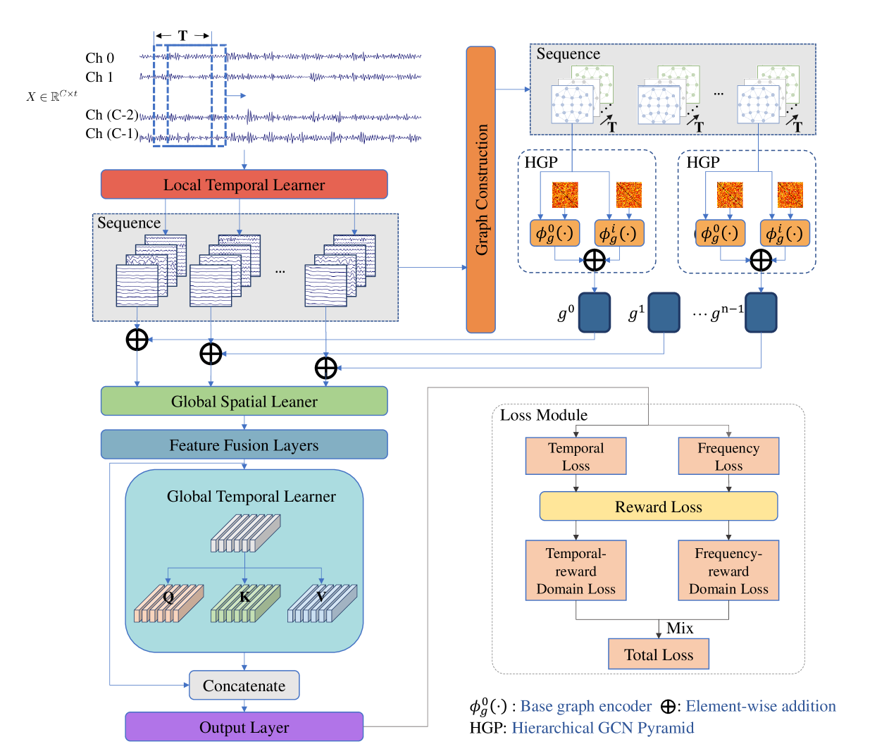
Figure 1: Overview of EEG2GAIT Architecture and Loss Calculation. The sequential EEG signals are segmented into training samples $X\in\mathbb{R}^{C\times T}$, where $C$ is the number of channels and $T$ is the time length. The Local Temporal Learner (LTL) uses 1D convolutions along the temporal dimension to capture local temporal information. The output is then reorganised into $n\times T$ temporal graphs, where $n$ is the number of samples. These graphs are input to the Hierarchical GCN Pyramid (HGP), which transforms each graph into a token embedding. The token for all graphs and the input for graph construction will be accumulated as input to the Global Spatial Learner (GSL). GSL performs 1D convolutions across all channels. The outputs are passed into the Feature Fusion Layers and then Global Temporal Learner (GTL) for global temporal information extraction via self-attention. The final output goes through the Output Layer. Losses from both the temporal (MSE) and frequency (FFT-based L1) domains are combined via a Reward Loss block to yield the Hybrid Temporal-Spectral Reward Loss.

3.2 Local Temporal Learner

Let a time-series EEG signal be denoted as $(X,Y)$, where $X\in\mathbb{R}^{C\times t}$ represents the EEG signal sampled at 100 Hz, and $Y\in\mathbb{R}^{d_{J}\times t}$ denotes the corresponding label, with $C$ denoting the number of channels, $t$ the total number of recorded time points, and $d_{J}$ representing the number of lower-limb joint angles. Subsequently, a sliding window of length $T$ and step size 1 is applied to further segment the signal into shorter subsequences. As a result, $X$ is divided into $(t-T+1)$ samples, denoted individually as $\bar{X}\in\mathbb{R}^{C\times T}$. Each $\bar{X}$ corresponds to a label $\bar{y}\in\mathbb{R}^{d_{J}}$.

We apply a one-dimensional convolution in the time domain on $\bar{X}$ to capture local temporal features. Specifically, we employ $F$ convolutional kernels with a size of $(1,10)$. In this experiment, $F$ is fixed at $25$, meaning $25$ temporal filters are applied to extract meaningful temporal patterns from the EEG signal. To ensure the input and output sizes remain consistent, zero-padding is applied along the time dimension, allowing the convolution to maintain the same temporal resolution as the input.

3.3 Graph Construction Module

Given the output of the Local Temporal Learner, denoted as $\bar{X}\in\mathbb{R}^{F\times C\times T}$, where $F$, $C$, and $T$ represent the number of feature maps, the number of EEG channels, and the time window length respectively, the Graph Construction Module transforms $\bar{X}$ into a temporal graph representation. In this graph representation, each EEG channel is treated as a graph node, and the spatial relationships between channels are encoded as graph edges.

The adjacency matrix $A\in\mathbb{R}^{C\times C}$ defines the connectivity between the EEG channels (nodes). The initial values of $A$ are determined by retaining neighboring channels within a 30 mm radius for each EEG channel. This approach ensures that only spatially close channels are connected, reflecting the localized relationships between EEG electrodes on the scalp. The resulting adjacency matrix captures the underlying spatial structure of the EEG data effectively.

To enhance the flexibility of the graph representation, the adjacency matrix is treated as a learnable parameter during training. This dynamic learning process allows the model to adaptively adjust the connections between channels, capturing task-specific spatial relationships inherent in the EEG signals. The updated adjacency matrix $\tilde{A}$ at any training step is computed as:

$$\tilde{A}=\text{ReLU}(A+A^{\top})+I,$$

where $I$ is the identity matrix representing self-loops, and ReLU ensures non-negative edge weights.

The constructed graph representation is then passed to the HGP for multi-level spatial embedding extraction. This process enables the model to dynamically integrate both predefined and learned spatial dependencies, effectively encoding the spatial relationships among EEG channels.

3.4 Hierarchical GCN Pyramid

We propose a Hierarchical GCN Pyramid (HGP) to modulate the dynamic spatial relationships between EEG channels associated with lower limb motor processes. For each output from the Local Temporal Learner, the shape is $(F,C,T)$. The Graph Construction Module reshapes sample $\bar{X}$ into $(T,C,F)$. Each channel is regarded as one node and extracted features $f\in\mathbb{R}^{F}$ are regarded as node attributes.

The HGP learns embedding $g^{i}$ for each subgraph $\hat{{X_{i}}}\in\mathbb{R}^{C\times F}$ to capture spatial features of the signal. A base graph encoder $\Phi_{g}(\cdot)$ is utilized to learn graph representations. In this paper, we use GCN [32] as the base graph encoder:

$$\Phi_{g}(\mathbf{H}^{(l+1)},\mathbf{A})=\sigma\left(\tilde{\mathbf{D}}^{-\frac{1}{2}}\tilde{\mathbf{A}}\tilde{\mathbf{D}}^{-\frac{1}{2}}\mathbf{H}^{(l)}\mathbf{W}^{(l)}+\mathbf{b}^{(l)}\right),$$

where:

• $\mathbf{H}^{(l)}$ represents the input node features at layer $l$, with $\mathbf{H}^{(0)}=\mathbf{X}$ as the initial node features;

• $\tilde{\mathbf{A}}=\mathbf{A}+\mathbf{I}$ is the adjacency matrix with added self-loops;

• $\tilde{\mathbf{D}}$ is the degree matrix of $\tilde{\mathbf{A}}$, i.e., $\tilde{D}_{ii}=\sum_{j}\tilde{A}_{ij}$;

• $\mathbf{W}^{(l)}$ is the trainable weight matrix at layer $l$;

• $\mathbf{b}^{(l)}$ is the bias term at layer $l$;

• $\sigma(\cdot)$ is the activation function, ReLU in this work.

In practice, $\tilde{\mathbf{D}}^{-\frac{1}{2}}\tilde{\mathbf{A}}\tilde{\mathbf{D}}^{-\frac{1}{2}}$ represents the normalized adjacency matrix, which is used to preserve the scale of feature representations after each graph convolution.

To modulate the diversity of brain region connections for different cognitive processes, we propose to use multiple hierarchical GCNs, i.e., $\{\Phi^{0}_{g}(\cdot),\Phi^{1}_{g}(\cdot),\dots,\Phi^{i}_{g}(\cdot)\}$, with learnable adjacency matrices $\{A^{0},A^{1},\dots,A^{i}\}$. Each $A^{i}$ learns the graph connections corresponding to a particular cognitive process. For each $\Phi^{i}_{g}(\cdot)$, stacking different GCN layers allows learning different levels of node cluster similarity. Intuitively, for localized connections, such as electrodes within the same brain functional area, a deeper GCN can achieve consistent representations among these nodes. However, for global connections across different brain regions, a shallower GCN can aggregate information between these areas without oversmoothing. The deeper $\Phi^{i}_{g}(\cdot)$ becomes, the higher the level in the feature pyramid its output represents.

3.5 Global Spatial Learner

The output from the HGP, consisting of two graph encoders, is first integrated with the original features through a residual connection. This step combines refined spatial embeddings with the initial features to prepare the data for subsequent processing by the Global Spatial Learner (GSL).

The GSL processes these combined features using a depth-wise grouped convolution[39] with a kernel size of $(C,1)$. This operation efficiently learns spatial filters specific to each temporal filter, enabling the extraction of frequency-specific spatial patterns. To further enhance the feature representations, batch normalization[40] is applied along the feature map dimension, followed by an exponential linear unit (ELU)[41] activation function. Dropout[42] with a probability of 0.5 is used to prevent overfitting when training on small datasets. Finally, an average pooling layer of size $(1,3)$ reduces the temporal resolution. As a result, the output size of the GSL is $(25,1,T//3)$.

3.6 Feature Fusion Layers

The Feature Fusion Layers refine spatial-temporal features through a series of convolutional blocks, consisting of three sequential convolutional blocks followed by a dropout layer. Each convolutional block applies the following operations: dropout (rate 0.5), zero-padding, convolution, batch normalization, ELU activation, and max-pooling. The kernel size and pooling size are consistent across all layers, while the number of filters varies to progressively increase feature complexity.

The first convolutional block uses 50 filters, followed by 100 and 200 filters in the second and third blocks, respectively. The kernel size is fixed at $(1,10)$ across all blocks, with zero-padding applied to maintain the temporal dimension. Each max-pooling operation reduces the temporal resolution by a factor of $1/3$, progressively compressing the time dimension of the data.

After the three convolutional blocks, the output passes through a dropout layer with a rate of 0.5 to mitigate overfitting. The final output of the Feature Fusion Layers has a size of $(200,1,T//81)$, ready for subsequent temporal modeling.

3.7 Global Temporal Learner

The Global Temporal Learner (GTL) captures temporal dynamics using a Multi-head Self-Attention (MSA) mechanism[43], which preserves the input-output shape consistency for efficient processing. Residual connections are employed to maintain the integrity of the input data and ensure stable gradient flow during training.

The input to the GTL is a tensor $X_{\text{spatial}}$ with shape $(200,T//81)$, representing the spatial-temporal features extracted from previous layers. To model temporal dependencies, $X_{\text{spatial}}$ is transformed into query ($Q_{i}$), key ($K_{i}$), and value ($V_{i}$) matrices for each attention head, where $Q_{i}$, $K_{i}$, and $V_{i}$ have dimensions $(n,d_{K})$. The self-attention mechanism for the $i$-th head is computed as:

$$\text{head${}_{i}$}=\text{softmax}\left(\frac{Q_{i}\cdot K_{i}^{T}}{\sqrt{d_{K}}}\right)V_{i}\quad(4)$$

The outputs from all attention heads are concatenated along the feature dimension and passed through a linear layer to generate the final attention representation:

$$X_{\text{attention}}=\text{linear}(\text{Concat}(\text{head}_{1},\ldots,\text{head}_{h}))\quad(5)$$

Here, $N_{\text{head}}$ is the number of attention heads, $d_{K}$ is the output dimension of each attention head, and $d_{\text{model}}$ is the final feature dimension after projection.

The self-attention mechanism evaluates pairwise correlations between the query and key representations of all time segments, enabling the model to effectively capture interdependencies across time. The output of the GTL has the same shape as its input, $(200,T//81)$, ensuring that the temporal features are preserved while enriching the representation with inter-segment dependencies.

3.8 Output Layer

The Output Layer generates the final predictions by processing the features extracted by the previous modules. The output of the GTL is concatenated with the original input along the temporal dimension, resulting in a tensor of shape $(200,T//81\times 2)$. Each sample is then unsqueezed to add a channel dimension, forming a tensor of shape $(200,1,T//81\times 2)$, which is passed to the Output Layer.

The Output Layer consists of a convolutional layer with $d_{J}$ kernels, each of size $(1,T//81\times 2)$. This operation reduces the temporal dimension while mapping the features to the desired output space. Finally, the tensor is reshaped by removing redundant dimensions, producing the final output with a shape of $(B,d_{J})$, where $B$ and $d_{J}$ corresponds to batch size and the number of joint angles predicted, respectively.

3.9 Loss Calculation Module

Given the model’s predictions $\hat{y}(t)$ and the ground truth $y(t)$, the total loss is composed of a time-domain loss and a frequency-domain loss, which are weighted and combined.

3.9.1 Time-Domain Loss

The time-domain loss is calculated using the MSE loss:

$$L_{\text{time}}=\frac{1}{n}\sum_{i=1}^{n}\left(\hat{y}_{i}-y_{i}\right)^{2}$$

To incentivize further learning from well-predicted samples, an additional Reward Loss term is introduced, defined as:

$$L_{\text{time\_reward}}=L_{\text{time}}+\beta\cdot\log\left(1-e^{-L_{\text{time}}}+\epsilon\right)$$

where $\beta$ is a weighting factor for the reward term, and $\epsilon$ is a small constant to avoid numerical instability (e.g., $\log(0)$).

3.9.2 Frequency-Domain Loss

To capture frequency-domain characteristics of the signal, the predictions and ground truth are transformed using the Discrete Fourier Transform (DFT). The frequency-domain error is computed using the $L1$ loss:

$$L_{\text{freq}}=\frac{1}{n}\sum_{i=1}^{n}\left|\hat{Y}_{i}-Y_{i}\right|$$

where $\hat{Y}(f)=\text{DFT}(\hat{y}(t))$ and $Y(f)=\text{DFT}(y(t))$ are the predicted and true signals in the frequency domain. Similar to the time-domain loss, an Encouraging Loss term is applied:

$$L_{\text{freq\_reward}}=L_{\text{freq}}+\beta\cdot\log\left(1-e^{-L_{\text{freq}}}+\epsilon\right)$$

3.9.3 HTSR Loss

The final Temporal-Spectral Reward (HTSR) loss function is a weighted combination of the time-domain and frequency-domain losses:

$$L_{\text{total}}=\alpha\cdot L_{\text{freq\_reward}}+(1-\alpha)\cdot L_{\text{time\_reward}}$$

where $\alpha$ controls the relative importance of the frequency-domain and time-domain losses. In this work, $\alpha$ is set to $0.5$, and $\beta$ is set to $0.1$.

4 Experiment

4.1 Dataset

4.1.1 Gait-EEG Dataset

To investigate the brain mechanisms involved in walking, we collected a new dataset, Gait-EEG Dataset (GED), recording brain activity along with simultaneous lower-limb joint angles natural walk on level ground. The dataset contains the recordings from 50 able-bodied participants (25 males, 25 females; aged 21 to 46, mean age 28.4, standard deviation 5.2), with no history of neurological disorders or lower limb pathologies. Participants engaged in two independent level-ground walking experiment sessions, with every session comprising three identical walking blocks. Each block included approximately 40 trials, with each trial representing EEG signals and synchronized lower-limb joint angles as the participant walked straight for 7.7 meters. The experiment protocol for each block is shown in Fig. 2. Sessions were spaced at least three days apart. The dataset includes synchronized recordings from a 60-channel active EEG, a 4-channel electrooculogram (EOG), along with measurements from six joint angle sensors (bilateral hips, knees, and ankles).

This study has been reviewed and approved by the Institutional Review Board (IRB-2021-709) of Nanyang Technological University, ensuring compliance with applicable legislation, ethical and safety requirements in Singapore. All participants have provided informed consents before the experiment.

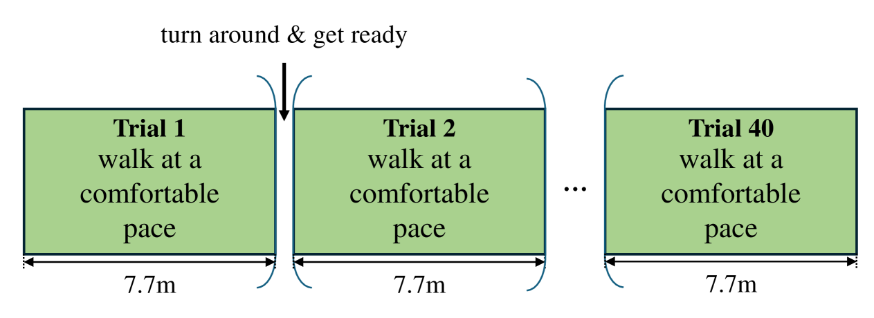
Figure 2: Experiment protocol for one block.

4.1.2 Open-access Dataset

To further validate our proposed method, we also conducted experiments using an open-access dataset, Mobile Brain-body imaging(MoBI) dataset[44]. The MoBI dataset includes recordings from eight participants across three sessions each. For each session, participants walked at a constant speed on a treadmill for a total of 20 minutes. During the first 15 minutes, participants received real-time feedback of their gait via an on-screen avatar mirroring their actual movements. In the final 5 minutes, the avatar’s gait feedback was driven by decoded EEG signals.

4.2 Data Preprocessing

Prior to analysis, the EEG data from both datasets underwent the same preprocessing steps. Initially, a minimum-phase filter was employed for band-pass filtering between 0.1 and 48 Hz. Subsequently, a common average reference was applied. The data were then downsampled from 100 Hz, followed by Independent Component Analysis (ICA). All components obtained from ICA were subjected to the computation of five metrics[45]: Spatial Average Difference, Spatial Eye Difference, Generic Discontinuities Spatial Feature, Maximum Epoch Variance, and Temporal Kurtosis.

A threshold for each metric was determined through maximum likelihood estimation. If any of the five metrics for a given component exceeded three times the threshold, that component was discarded. On average, 8.96 components were removed for each session in GED and 9.54 components were removed for each session in MoBI. Subsequently, the data from the EOG channels were removed, resulting in a final EEG dataset consisting of 59 channels for GED and MoBI dataset.

Finally, a local Laplacian filtering was applied to enhance local activity within a specified area. It achieves this by computing the differences between the values of the target channel and the average of values from its neighbor channels. For each EEG channel, neighboring channels within a 30 mm radius are retained as its neighbors. This method effectively emphasizes the local features and diminishes the interference from distant sources. The mathematical representation of the local Laplacian filtering process is given by the following formula:

$$V^{\prime}_{k}=V_{k}-\frac{1}{N}\sum_{l=1}^{N}V_{l}$$ (1)

where:

• $V^{\prime}_{k}$ is the value of the $k^{th}$ channel after applying the Laplacian filter.

• $V_{k}$ is the original value at the $k^{th}$ channel.

• $N$ is the number of neighbors used for calculating the average.

• $V_{l}$ represents the original values of the surrounding channels.

4.3 Data Segregation

4.3.1 Gait-EEG Dataset

The last 20 trials of the third block were divided, with the first 5 trials serving as the validation set and the subsequent 15 trials being concatenated along the time dimension to build the test set, while the remaining trials formed the training set. Since EEG2GAIT is a session-specific model, we separately trained EEG2GAIT models using training sets from each session and tested them with the test sets from their respective sessions.

4.3.2 MoBI Dataset

For each session, we use the first 15 minutes of walking data without closed-loop BCI control as the training set and the last 5 minutes of walking data with closed-loop BCI control as the test set. Additionally, the last 10% of the training set, which is the final 1.5 minutes of data, is set aside as the validation set.

4.4 Evaluation Metric

We evaluated the efficacy of EEG2GAIT by comparing the predicted angles of six joints with their actual recorded angles, using their correlation ($r$ value) and coefficient of determination ($R^{2}$ score) as the evaluation metrics:

$$r=\frac{\operatorname{cov}(y,\hat{y})}{\sigma(y)\cdot\sigma(\hat{y})}$$ (2)

$$R^{2}=1-\frac{\sum_{i=1}^{n}\left(y_{i}-\hat{y}_{i}\right)^{2}}{\sum_{i=1}^{n}\left(y_{i}-\bar{y}\right)^{2}}$$ (3)

where $y$ denotes the actual joint angle, and $\hat{y}$ represents the predicted angle. The covariance between any two variables A and B is expressed as $cov(A,B)$, while $\sigma(A)$ signifies the standard deviation of A. Each sequence represents the data collected from a single trial, capturing the observations over a specific period. In this case, the sequence contains $n$ data points, which corresponds to $\frac{n}{100}$ seconds of data, given that the data was sampled at a frequency of 100 Hz. $\hat{y}_{i}$ refers to the value at the $i^{th}$ position. Lastly, $\bar{y}$ stands for the average of the actual joint angles. The $r$ value reflects the consistency in trend between the predicted and actual gait. The $R^{2}$ score reflects the second-order absolute error between the predicted and actual gait, providing insight into the predictive performance of the model.

4.5 Implementation and Hyperparameter Settings

The EEG2GAIT model was implemented using the PyTorch library. Training was performed using the Adam optimizer with default hyperparameter settings, and the learning rate was fixed at 0.001. A batch size of 100 was used, and training continued for a maximum of 50 epochs ($epoch_{\text{max}}$). Early stopping was applied with a patience parameter ($p$) of 30 epochs, terminating training if the Pearson correlation coefficient ($r$) on the validation set did not improve for 30 consecutive epochs.

5 Results and Analysis

In this section, we validate the performance of the proposed method on the Gait-EEG dataset and MoBI dataset[44] and compared with several state-of-the-art deep learning and machine learning algorithms in the brain-computer interface (BCI) domain, including ContraWR[46], FFCL[47], TSception[48], Temporal Convolutional Network (TCN)[49], ST-Transformer[50], EEGConformer[51], SPaRCNet[52], EEGNet[14], and deepConvNet[13]. An ablation study was conducted to demonstrate the contributions of the HGP module and HTSR loss. Saliency mapping across EEG channels identified specific channels with notably higher contributions to the decoding task, offering a spatial interpretation of the neural correlates involved in lower-limb motor decoding as well as validating the obtained features. This confirms that the model effectively leverages signals from motor-related areas. Additionally, we illustrate the overlay of decoding results across different models for the gait cycle, offering a more intuitive display of EEG2GAIT’s superior performance.

Fig. 3 illustrates the visualization of the predicted and actual knee joint angles for the left knee during the test set of participant 2’s second session ($r$ = $0.962$, $R^{2}$ = $0.918$). The gait cycles were segmented using peak detection on the goniometer-measured angles, with each peak representing a boundary between consecutive gait cycles. The segment between two consecutive peaks was defined as a single gait cycle, which was subsequently interpolated to a fixed length of 400 time points for standardization.

The blue solid line represents the mean goniometer-measured angle for each time point across all gait cycles, while the blue shaded region indicates the standard deviation of the measured values, reflecting variability across gait cycles. The red dashed line shows the predicted mean knee joint angle at each time point, and the red shaded region depicts the predicted standard deviation.

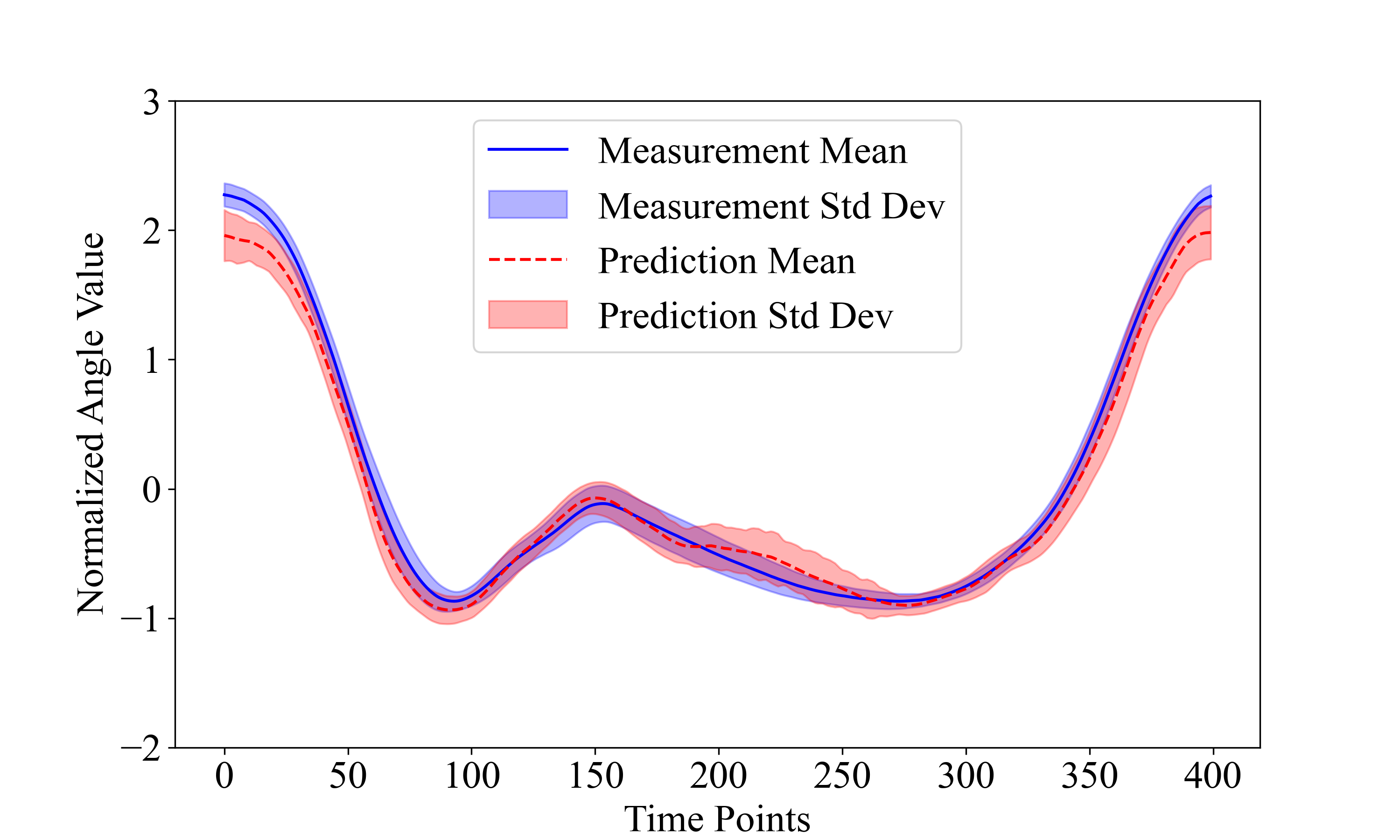
Figure 3: Visualization of the actual and predicted left knee joint angles for the test set in participant 2’s second session. The goniometer-measured angles were segmented into gait cycles using peak detection, with each gait cycle interpolated to 400 time points. The blue solid line represents the actual mean angle, and the blue shaded area indicates the standard deviation of the measured angles across all gait cycles. The red dashed line denotes the predicted mean angle, while the red shaded area shows the standard deviation of the predictions.

5.1 Model Performance

The results of all metrics on the test sets are presented to evaluate the performance of EEG2GAIT in comparison to baseline methods on the MoBI and GED dataset. EEG2GAIT achieved an $r$ value of 0.935 ($R^{2}$ = 0.865) on the GED dataset with 50 subjects and an $r$ value of 0.713 ($R^{2}$ = 0.484) on the MoBI dataset with 8 subjects, outperforming the baseline methods. All baseline methods were trained according to the strategy described in Section 4.3. A summary of the results for EEG2GAIT and the baseline methods on the different datasets is provided in Table 1 and 2. Overall, EEG2GAIT demonstrated the best performance across all metrics among all methods, with a lower standard deviation than most methods.

Table 1: Prediction performance of different models on the MoBI dataset, indicated by mean $\pm$ standard deviation of the correlations ($r$) and coefficients of determination ($R^{2}$) between predictions and true signals, averaged over the six joints. The symbol $\pm$ indicates the mean value followed by its standard deviation. The highest mean value in each column is marked in bold, while the lowest standard deviation in each column has been underlined.

Model Name	$r$ value	$R^{2}$ score
ContraWR[46]	0.314$\pm$0.1693	0.0427$\pm$0.1117
FFCL[47]	0.4407$\pm$0.1996	0.1413$\pm$0.2285
TSception[48]	0.5527$\pm$0.1982	0.1918$\pm$0.3661
TCN[49]	0.6099$\pm$0.1658	0.3423$\pm$0.2396
ST-Transformer[50]	0.676$\pm$0.1996	0.4099$\pm$0.3183
EEGConformer[51]	0.6027$\pm$0.1948	0.3325$\pm$0.2816
SPaRCNet[52]	0.6459$\pm$0.2219	0.3586$\pm$0.3677
EEGNet[14]	0.6495$\pm$0.2063	0.3988$\pm$0.2848
deepConvNet[13]	0.6854$\pm$0.1969	0.4539$\pm$0.3059
EEG2GAIT(w/o HGP)	0.7009$\pm$0.1822	0.4517$\pm$0.3337
EEG2GAIT	0.7126$\pm$0.1799	0.4835$\pm$0.304

Table 2: Prediction performance of different models on the on GED, indicated by mean $\pm$ standard deviation, averaged over the six joints. The highest mean value in each column is marked in bold, while the highest mean value in each row is marked with a superscript star (*). The lowest standard deviation in each column has been underlined.

$r$ value results:
Model Name\Loss Functions $L_{MSE}$ $L_{time+freq}$ $L_{time\_reward}$ $L_{HTSR}$ ContraWR[46] 0.6056$\pm$0.2342 0.6191$\pm$0.2284 0.6129$\pm$0.2375 0.6263^∗$\pm$0.2219 FFCL[47] 0.654$\pm$0.2107 0.666$\pm$0.2013 0.6623$\pm$0.209 0.671^∗$\pm$0.2003 TSception[48] 0.6866$\pm$0.1418 0.7114$\pm$0.135 0.7084$\pm$0.1378 0.7257^∗$\pm$0.1284 TCN[49] 0.6737$\pm$0.1804 0.6968$\pm$0.1716 0.6857$\pm$0.1765 0.7034^∗$\pm$0.1702 ST-Transformer[50] 0.881$\pm$0.0892 0.8866$\pm$0.084 0.8846$\pm$0.0857 0.8898^∗$\pm$0.0834 EEGConformer[51] 0.861$\pm$0.1049 0.8683$\pm$0.099 0.8664$\pm$0.1016 0.8739^∗$\pm$0.0967 SPaRCNet[52] 0.8718$\pm$0.1042 0.884$\pm$0.0919 0.8832$\pm$0.0929 0.8877^∗$\pm$0.0891 EEGNet[14] 0.847$\pm$0.0947 0.86$\pm$0.0824 0.8604$\pm$0.0826 0.8641^∗$\pm$0.0782 deepConvNet[13] 0.9127$\pm$0.0729 0.9187$\pm$0.0595 0.9185$\pm$0.0608 0.9224^∗$\pm$0.0567 EEG2GAIT(w/o HGP) 0.922$\pm$0.0578 0.9235$\pm$0.0581 0.9239$\pm$0.0581 0.9257^∗$\pm$0.0537 EEG2GAIT 0.9301$\pm$0.0512 0.9338$\pm$0.0489 0.9337$\pm$0.0489 0.9351^∗$\pm$0.0477

$R^{2}$ score results:
Model Name\Loss Functions $L_{MSE}$ $L_{time+freq}$ $L_{time\_reward}$ $L_{HTSR}$ ContraWR[46] 0.2788$\pm$0.3369 0.3114$\pm$0.3472 0.3243$\pm$0.3343 0.3142^∗$\pm$0.349 FFCL[47] 0.3874$\pm$0.3027 0.3958$\pm$0.299 0.3981$\pm$0.306 0.4046^∗$\pm$0.2945 TSception[48] 0.4022$\pm$0.3195 0.4437$\pm$0.3821 0.4407$\pm$0.3293 0.4813^∗$\pm$0.2584 TCN[49] 0.4528$\pm$0.2469 0.4827$\pm$0.2488 0.4694$\pm$0.2476 0.4914^∗$\pm$0.2427 ST-Transformer[50] 0.7512$\pm$0.1716 0.7612$\pm$0.1625 0.7595$\pm$0.1633 0.7681^∗$\pm$0.1587 EEGConformer[51] 0.7383$\pm$0.1732 0.7483$\pm$0.1705 0.7461$\pm$0.1726 0.7597^∗$\pm$0.1618 SPaRCNet[52] 0.7252$\pm$0.2027 0.7453$\pm$0.1879 0.744$\pm$0.1859 0.7534^∗$\pm$0.1809 EEGNet[14] 0.688$\pm$0.1797 0.7086$\pm$0.156 0.71$\pm$0.1547 0.715^∗$\pm$0.1534 deepConvNet[13] 0.8147$\pm$0.1571 0.8293$\pm$0.1099 0.8291$\pm$0.1127 0.8375^∗$\pm$0.1061 EEG2GAIT(w/o HGP) 0.8406$\pm$0.1083 0.8448$\pm$0.1073 0.8461$\pm$0.1066 0.8487^∗$\pm$0.0999 EEG2GAIT 0.8553$\pm$0.0965 0.8624$\pm$0.0938 0.8629$\pm$0.0922 0.8651^∗$\pm$0.092

5.2 Ablation Analysis

The results of the loss ablation studies can be observed across the columns in Table 2. The HTSR loss, our proposed composite loss function combining frequency-domain loss, time-domain loss, and reward module, demonstrated superior performance compared to MSE loss across all baseline models and our EEG2GAIT model ($p\ll 0.01$ (Bonferroni corrected for 2 evaluated metrics and 11 models), paired-sample t-test, one-tail). Furthermore, as we progressively isolated each component of the loss function, the results showed that each individual component contributed positively to model performance for most models.

The HGP ablation study results can be found in the last two rows of tables in Table 1 and 2. When the HGP module was removed, the performance of EEG2GAIT declined. However, it still outperformed all baseline models, demonstrating the robustness and effectiveness of the core framework even without the HGP module.

5.3 Spatial Analysis

In addition to the performance metrics presented, we expanded our evaluation to include spatial feature importance analysis to better understand critical areas during decoding. To achieve this, we employed saliency mapping—a technique in machine learning that visualizes the importance of each input feature for the model’s predictions[53]. This method highlights the input areas the model is most sensitive to when making predictions. The saliency map, $S$, is generated by calculating the gradient of the model’s output with respect to each input feature. The gradients are visualized to represent how variations in each input element, $X_{ij}$ (where $i,j$ are the spatial and temporal indices of $X$ , an input sample in $\mathbf{R}^{C\times T}$), influence the output prediction. The magnitude of each element $S_{ij}$ in $S$ illustrates the importance of the corresponding input pixel $X_{ij}$ to the output prediction.

To derive a spatial saliency map from these calculations, we first averaged $S$ across the temporal dimension to obtain $\bar{S}$. We then projected $\bar{S}$ onto the corresponding scalp electrode positions by averaging across all time points of $S$, creating a topographical map that illustrates the focal areas of brain activity relevant to the model’s decisions.

The saliency maps are plotted in Figure 4. The results indicated that the highlighted EEG channels during subjects’ walking were concentrated in the motor areas, especially in the lower-limb area, which is the anterior paracentral area[54]. Our observations consistently pointed towards the motor areas, particularly channel Cz, FC1, FC2, Fz, CP1, CP2, exhibiting notably higher saliency compared to other regions. As shown in Figure 4, the average saliency maps across all subjects indicate strong role of central motor region in gait pattern encoding.

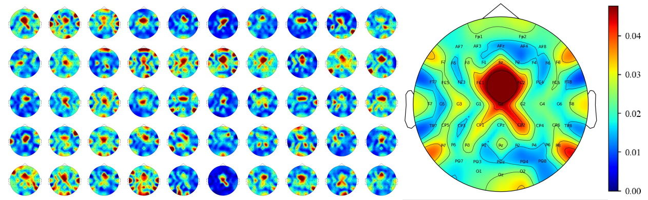
Figure 4: Saliency maps generated by EEG2GAIT: (a) individual saliency maps for each subject, and (b) the average saliency map computed across all subjects.

6 Discussion

In our current work, we proposed EEG2GAIT, a novel hierarchical graph neural network model specifically designed to address the limitations of existing approaches, which often fail to fully explore neurophysiological priors, thereby neglecting the spatial relationships between individual recording channels. Comparisons with state-of-the-art models demonstrated that EEG2GAIT achieves superior performance on two independent gait datasets. A novel loss function was introduced to leverage the temporal and spectral information inherent in EEG recordings and mitigate the limitations of existing loss functions. Feature importance analyses finally highlighted the considerable contributions of cortical regions known to be involved in gait generation, thereby providing neurophysiological validation for the obtained results.

6.1 Hierarchical Graph Convolutional Network Pyramid

The proposed Hierarchical Graph Convolutional Network Pyramid (HGP) introduced a novel framework for capturing spatial relationships among EEG channels associated with gait-related brain activity by modeling EEG signals as a non-Euclidean structure. Direct comparison with existing state-of-the-art models in EEG-decoding revealed superior performance of the proposed approach, both in terms of achieved correlation and $R^{2}$-score between prediction and ground truth, and in the corresponding standard deviations (see Table 2). Importantly, the use of hierarchical graph convolutional layers with learnable adjacency matrices displayed the best regression performance of all compared methods, showing slight improvement compared to the basic EEG2Gait model without the hierarchical graph convolutional network (GCN) pyramid (HGP), specifically in the $R^{2}$-score. These findings stands in line with previous research, which documented effective motor activity decoding during gait by leveraging hierarchical graph convolutional layers with learnable adjacency matrices[55, 56].

The reported performance of EEG2GAIT in aligning predicted and actual gait sequences within different datasets (see Tables 1 and 2) highlights its ability to model the neural underpinnings of gait with high fidelity. Specifically, the proposed model largely outperformed nine other state-of-the-art benchmark models specifically designed to decode information from ongoing EEG signals in terms of mean squared error between regressed and actual gait signals. As demonstrated in the ablation study (Table 2), we also compared the performance of EEG2GAIT without HGP. The results indicate that with the inclusion of HGP, EEG2GAIT achieves slightly enhanced performance in both the $r$ value and $R^{2}$ score dimensions, demonstrating that the addition of HGP consistently improves EEG2GAIT’s performance across all loss functions. Furthermore, the reduction in variance indicates that the inclusion of HGP makes the model’s performance more stable.

6.2 Combined temporal and spectral losses

The proposed Hybrid Temporal-Spectral Reward (HTSR) Loss addresses key challenges in continuous gait decoding from EEG by combining time-domain, frequency-domain, and reward mechanisms. As shown in Table 2, the use of time- and frequency-domain information (second column) consistently improved both correlations and $R^{2}$-score across the regarded models when only using a MSE loss (first column). Likewise, consistent performance improvements emerged when rewarding accurate inferences via a temporal reward loss (third column) compared to an ordinary MSE loss (first column), indicating that learning from correct examples, as opposed to the traditional approach of learning via penalties, indeed improves the models performance. Interestingly, combining the two approaches to our proposed hybrid temporal-spectral reward (HTSR) loss yielded superior performance across all models. The performance improvement most likely stems from the fact that the hybrid framework enhances the model’s ability to capture subtle temporal patterns and long-term contextual information for decoding. Specifically, the time-domain loss ensures accurate gait prediction, while the reward mechanism preserves fine-grained temporal details. Additionally, the frequency-domain component, leveraging the Discrete Fourier Transform (DFT), effectively captures long-term dependencies, with a reward term that emphasizes key spectral features. Overall, the HTSR loss outperforms the conventional MSE loss function, demonstrating its efficacy in addressing the unique challenges of time-series modeling (see Table 2).

6.3 Saliency Map Insights into Cortical Dynamics

Feature importance analysis using saliency maps revealed a consistent focus on sagittal-line electrodes in the frontocentral region, particularly around Cz, FC1, FC2, Fz, CP1, and CP2. These electrodes correspond to the bilateral leg motor area, aligning with prior findings on the neural representation of lower-limb motor control[57, 58]. The consistency of these results across participants underscores the neurophysiological relevance and generalizability of the extracted features, confirming the model’s robustness against individual variations in head physiology.

7 Conclusion

In this work, we proposed a hierarchical graph-based model, EEG2GAIT, for decoding gait dynamics from EEG signals. The model integrates a Hierarchical GCN Pyramid for spatial feature extraction with a Hybrid Temporal-Spectral Reward (HTSR) Loss to capture intricate temporal and spectral features. We also contributed a new Gait-EEG dataset. Experiments on the GED dataset and the publicly available MoBI dataset demonstrated that EEG2GAIT surpasses state-of-the-art methods in accuracy and robustness for joint angle prediction. Ablation studies validated the contributions of the HGP module and HTSR Loss, while saliency map analyses highlighted the spatial correlates of motor decoding, underscoring the importance of central motor regions. These results demonstrate the potential of EEG-based gait decoding for advancing brain-computer interface (BCI) applications in neurorehabilitation and assistive technologies.

Future studies could extend the dataset to diverse populations and explore adaptive graph structures and attention mechanisms to improve decoding of complex neural patterns.

References

- [1] Richard A Schmidt et al. “Motor control and learning: A behavioral emphasis” Human kinetics, 2018
- [2] Gert Pfurtscheller and A Aranibar “Event-related cortical desynchronization detected by power measurements of scalp EEG” In Electroencephalography and clinical neurophysiology 42.6 Elsevier, 1977, pp. 817–826
- [3] Po T Wang et al. “Self-paced brain–computer interface control of ambulation in a virtual reality environment” In Journal of neural engineering 9.5 IOP Publishing, 2012, pp. 056016
- [4] Paul Dominick E Baniqued et al. “Brain–computer interface robotics for hand rehabilitation after stroke: a systematic review” In Journal of neuroengineering and rehabilitation 18 Springer, 2021, pp. 1–25
- [5] Zhengzhe Cui et al. “BCI system with lower-limb robot improves rehabilitation in spinal cord injury patients through short-term training: a pilot study” In Cognitive Neurodynamics 16.6 Springer, 2022, pp. 1283–1301
- [6] Juan Pablo Romero et al. “Clinical and neurophysiological effects of bilateral repetitive transcranial magnetic stimulation and EEG-guided neurofeedback in Parkinson’s disease: a randomized, four-arm controlled trial” In Journal of NeuroEngineering and Rehabilitation 21.1 Springer, 2024, pp. 135
- [7] Kai Keng Ang, Zheng Yang Chin, Haihong Zhang and Cuntai Guan “Filter bank common spatial pattern (FBCSP) in brain-computer interface” In 2008 IEEE international joint conference on neural networks (IEEE world congress on computational intelligence), 2008, pp. 2390–2397 IEEE
- [8] Hiroshi Higashi and Toshihisa Tanaka “Common Spatio-Time-Frequency Patterns for Motor Imagery-Based Brain Machine Interfaces” In Computational intelligence and neuroscience 2013.1 Wiley Online Library, 2013, pp. 537218
- [9] Álvaro Costa et al. “Decoding the attentional demands of gait through EEG gamma band features” In PLoS one 11.4 Public Library of Science San Francisco, CA USA, 2016, pp. e0154136
- [10] Minmin Miao, Aimin Wang and Feixiang Liu “A spatial-frequency-temporal optimized feature sparse representation-based classification method for motor imagery EEG pattern recognition” In Medical & biological engineering & computing 55 Springer, 2017, pp. 1589–1603
- [11] José-Vicente Riquelme-Ros et al. “On the better performance of pianists with motor imagery-based brain-computer interface systems” In Sensors 20.16 MDPI, 2020, pp. 4452
- [12] Ping Wang et al. “LSTM-based EEG classification in motor imagery tasks” In IEEE transactions on neural systems and rehabilitation engineering 26.11 IEEE, 2018, pp. 2086–2095
- [13] Robin Tibor Schirrmeister et al. “Deep learning with convolutional neural networks for EEG decoding and visualization” In Human brain mapping 38.11 Wiley Online Library, 2017, pp. 5391–5420
- [14] Vernon J Lawhern et al. “EEGNet: a compact convolutional neural network for EEG-based brain–computer interfaces” In Journal of neural engineering 15.5 iOP Publishing, 2018, pp. 056013
- [15] Pranav G Reddy et al. “Brain state flexibility accompanies motor-skill acquisition” In NeuroImage 171 Elsevier, 2018, pp. 135–147
- [16] Gert Pfurtscheller and FH Lopes Da Silva “Event-related EEG/MEG synchronization and desynchronization: basic principles” In Clinical neurophysiology 110.11 Elsevier, 1999, pp. 1842–1857
- [17] Christa Neuper and Gert Pfurtscheller “Event-related dynamics of cortical rhythms: frequency-specific features and functional correlates” In International journal of psychophysiology 43.1 Elsevier, 2001, pp. 41–58
- [18] Josje M Bootsma et al. “Neural correlates of motor skill learning are dependent on both age and task difficulty” In Frontiers in aging neuroscience 13 Frontiers Media SA, 2021, pp. 643132
- [19] Han Yuan et al. “Negative covariation between task-related responses in alpha/beta-band activity and BOLD in human sensorimotor cortex: an EEG and fMRI study of motor imagery and movements” In Neuroimage 49.3 Elsevier, 2010, pp. 2596–2606
- [20] Trent J Bradberry, Rodolphe J Gentili and José L Contreras-Vidal “Reconstructing three-dimensional hand movements from noninvasive electroencephalographic signals” In Journal of neuroscience 30.9 Soc Neuroscience, 2010, pp. 3432–3437
- [21] Yimin Hou et al. “GCNs-net: a graph convolutional neural network approach for decoding time-resolved eeg motor imagery signals” In IEEE Transactions on Neural Networks and Learning Systems IEEE, 2022
- [22] Peixiang Zhong, Di Wang and Chunyan Miao “EEG-based emotion recognition using regularized graph neural networks” In IEEE Transactions on Affective Computing 13.3 IEEE, 2020, pp. 1290–1301
- [23] Gert Pfurtscheller and Christa Neuper “Motor imagery and direct brain-computer communication” In Proceedings of the IEEE 89.7 IEEE, 2001, pp. 1123–1134
- [24] Kai Keng Ang et al. “Filter bank common spatial pattern algorithm on BCI competition IV datasets 2a and 2b” In Frontiers in neuroscience 6 Frontiers Research Foundation, 2012, pp. 39
- [25] Sim Kuan Goh et al. “Spatio–spectral representation learning for electroencephalographic gait-pattern classification” In IEEE Transactions on Neural Systems and Rehabilitation Engineering 26.9 IEEE, 2018, pp. 1858–1867
- [26] Stefano Tortora et al. “Deep learning-based BCI for gait decoding from EEG with LSTM recurrent neural network” In Journal of neural engineering 17.4 IOP Publishing, 2020, pp. 046011
- [27] Xi Fu, Liming Zhao and Cuntai Guan “MATN: Multi-model Attention Network for Gait Prediction from EEG” In 2022 IEEE international joint conference on neural networks (IEEE world congress on computational intelligence), 2022, pp. 1–8 IEEE
- [28] Can Wang, Xinyu Wu, Zhouyang Wang and Yue Ma “Implementation of a brain-computer interface on a lower-limb exoskeleton” In IEEE access 6 IEEE, 2018, pp. 38524–38534
- [29] Joan Bruna, Wojciech Zaremba, Arthur Szlam and Yann LeCun “Spectral networks and locally connected networks on graphs” In arXiv preprint arXiv:1312.6203, 2013
- [30] Michaël Defferrard, Xavier Bresson and Pierre Vandergheynst “Convolutional neural networks on graphs with fast localized spectral filtering” In Advances in neural information processing systems 29, 2016
- [31] Ron Levie, Federico Monti, Xavier Bresson and Michael M Bronstein “Cayleynets: Graph convolutional neural networks with complex rational spectral filters” In IEEE Transactions on Signal Processing 67.1 IEEE, 2018, pp. 97–109
- [32] Thomas N Kipf and Max Welling “Semi-Supervised Classification with Graph Convolutional Networks” In International Conference on Learning Representations, 2022
- [33] Foroogh Shamsi, Ali Haddad and Laleh Najafizadeh “Early classification of motor tasks using dynamic functional connectivity graphs from EEG” In Journal of neural engineering 18.1 IOP Publishing, 2021, pp. 016015
- [34] Dalin Zhang, Kaixuan Chen, Debao Jian and Lina Yao “Motor imagery classification via temporal attention cues of graph embedded EEG signals” In IEEE journal of biomedical and health informatics 24.9 IEEE, 2020, pp. 2570–2579
- [35] Guangxiang Zhao et al. “Well-classified examples are underestimated in classification with deep neural networks” In Proceedings of the AAAI Conference on Artificial Intelligence 36.8, 2022, pp. 9180–9189
- [36] Sen Yang et al. “DeepNoise: signal and noise disentanglement based on classifying fluorescent microscopy images via deep learning” In Genomics, Proteomics and Bioinformatics 20.5 Oxford University Press, 2022, pp. 989–1001
- [37] Changhun Jung et al. “WBC image classification and generative models based on convolutional neural network” In BMC Medical Imaging 22.1 Springer, 2022, pp. 94
- [38] Hyun Kwon and Sanghyun Lee “Friend-guard adversarial noise designed for electroencephalogram-based brain–computer interface spellers” In Neurocomputing 506 Elsevier, 2022, pp. 184–195
- [39] Alex Krizhevsky, Ilya Sutskever and Geoffrey E Hinton “Imagenet classification with deep convolutional neural networks” In Advances in neural information processing systems 25, 2012
- [40] Sergey Ioffe and Christian Szegedy “Batch normalization: Accelerating deep network training by reducing internal covariate shift” In International conference on machine learning, 2015, pp. 448–456 pmlr
- [41] Djork-Arné Clevert, Thomas Unterthiner and Sepp Hochreiter “Fast and accurate deep network learning by exponential linear units (elus)” In International Conference on Learning Representations (ICLR), 2016
- [42] Nitish Srivastava et al. “Dropout: a simple way to prevent neural networks from overfitting” In The journal of machine learning research 15.1 JMLR. org, 2014, pp. 1929–1958
- [43] A Vaswani “Attention is all you need” In Advances in Neural Information Processing Systems, 2017
- [44] Yongtian He et al. “A mobile brain-body imaging dataset recorded during treadmill walking with a brain-computer interface” In Scientific data 5.1 Nature Publishing Group, 2018, pp. 1–10
- [45] Andrea Mognon, Jorge Jovicich, Lorenzo Bruzzone and Marco Buiatti “ADJUST: An automatic EEG artifact detector based on the joint use of spatial and temporal features” In Psychophysiology 48.2 Wiley Online Library, 2011, pp. 229–240
- [46] Chaoqi Yang, Danica Xiao, M Brandon Westover and Jimeng Sun “Self-supervised eeg representation learning for automatic sleep staging” In arXiv preprint arXiv:2110.15278, 2021
- [47] Hongli Li, Man Ding, Ronghua Zhang and Chunbo Xiu “Motor imagery EEG classification algorithm based on CNN-LSTM feature fusion network” In Biomedical signal processing and control 72 Elsevier, 2022, pp. 103342
- [48] Yi Ding et al. “Tsception: Capturing temporal dynamics and spatial asymmetry from EEG for emotion recognition” In IEEE Transactions on Affective Computing 14.3 IEEE, 2022, pp. 2238–2250
- [49] Thorir Mar Ingolfsson et al. “EEG-TCNet: An accurate temporal convolutional network for embedded motor-imagery brain–machine interfaces” In 2020 IEEE International Conference on Systems, Man, and Cybernetics (SMC), 2020, pp. 2958–2965 IEEE
- [50] Yonghao Song, Xueyu Jia, Lie Yang and Longhan Xie “Transformer-based spatial-temporal feature learning for EEG decoding” In arXiv preprint arXiv:2106.11170, 2021
- [51] Yonghao Song, Qingqing Zheng, Bingchuan Liu and Xiaorong Gao “EEG Conformer: Convolutional Transformer for EEG Decoding and Visualization” In IEEE Transactions on Neural Systems and Rehabilitation Engineering 31, 2023, pp. 710–719 DOI: 10.1109/TNSRE.2022.3230250
- [52] Jin Jing et al. “Development of expert-level classification of seizures and rhythmic and periodic patterns during eeg interpretation” In Neurology 100.17 AAN Enterprises, 2023, pp. e1750–e1762
- [53] Karen Simonyan, Andrea Vedaldi and Andrew Zisserman “Deep inside convolutional networks: Visualising image classification models and saliency maps” In arXiv preprint arXiv:1312.6034, 2013
- [54] Wilder Penfield and Edwin Boldrey “Somatic motor and sensory representation in the cerebral cortex of man as studied by electrical stimulation” In Brain 60.4 Citeseer, 1937, pp. 389–443
- [55] Biao Sun et al. “Adaptive spatiotemporal graph convolutional networks for motor imagery classification” In IEEE Signal Processing Letters 28 IEEE, 2021, pp. 219–223
- [56] Yunfa Fu et al. “Decoding of Motor Coordination Imagery Involving the Lower Limbs by the EEG-Based Brain Network” In Computational Intelligence and Neuroscience 2021.1 Wiley Online Library, 2021, pp. 5565824
- [57] Yuhang Zhang, Saurabh Prasad, Atilla Kilicarslan and Jose L Contreras-Vidal “Multiple kernel based region importance learning for neural classification of gait states from EEG signals” In Frontiers in neuroscience 11 Frontiers Media SA, 2017, pp. 170
- [58] Yuxuan Wei et al. “Decoding movement frequencies and limbs based on steady-state movement-related rhythms from noninvasive EEG” In Journal of Neural Engineering 20.6 IOP Publishing, 2023, pp. 066019